Vegetation Development in a Tidal Marsh Restoration Project during a Historic Drought: A Remote Sensing Approach

Introduction

Tidal wetland ecosystems worldwide are threatened by a range of human activities (Zedler and Kercher, 2005; Erwin, 2009; Klemas, 2013) and have been in steady decline for the last 150 years in California (Goals Project, 2015). In recent years, significant efforts have been undertaken to reverse this widespread loss and alteration. To effectively implement and plan restoration efforts, detailed understandings of system dynamics are necessary for driving adaptive management approaches (Spencer et al., 2016). To date, studies of restoration projects have focused more on the physical aspects of vegetation development and how they relate to sediment supply, initial elevation, and landscape context (Williams and Orr, 2002; Kelly et al., 2011; Brand et al., 2012). However, due to a variety of interacting factors, restoration projects may not proceed in a simple linear manner over time (Holmgren and Scheffer, 2001; Peters et al., 2004; Holmgren et al., 2006; Scheffer et al., 2009; Sitters et al., 2012; Chapple et al., 2017). Rates of restoration change over time and the factors that influence these transitions are critical yet understudied aspects of the restoration process. Since restoration projects increasingly use iterative, data-driven adaptive management strategies to plan projects, an improved understanding of how systems change over longer time periods is necessary.

Due to its Mediterranean-type climate and variable weather between years, California's San Francisco Bay (SF Bay) is an interesting location to study how climate variability influences restoration projects (Chapple et al., 2017). Between 2011 and 2015, California experienced an extreme drought event with an essentially incalculable return period (Robeson, 2015). This extended dry period has led to changes in other plant communities across the state (Asner et al., 2016; Copeland et al., 2016), and has likely influenced restoration project trajectories (Holmgren and Scheffer, 2001; Chapple et al., 2017). At the broad scale, plant communities in SF Bay tidal wetlands are primarily influenced by the salinity of tide waters (Malamud-Roam and Ingram, 2004; Callaway et al., 2007), which are influenced by snowpack levels and a complex series of upstream interactions across the state (Dettinger and Cayan, 2003). Anthropogenic sources of atmospheric carbon appear to be contributing to reduced snow pack in the state, which is expected to continue declining (Berg and Hall, 2017). These shifts will likely have major impacts on salinity and plant community dynamics throughout the estuary (Malamud-Roam and Ingram, 2004; Callaway et al., 2007) and will play a role in determining how restoration trajectories progress (Chapple et al., 2017). An improved understanding of how extreme events like California's historic drought impact restoration efforts is essential for future management (Holmgren and Scheffer, 2001; Holmgren et al., 2006; Callaway et al., 2007; Sitters et al., 2012; Zedler et al., 2012), given that increased climate variability is a major projected outcome of climate change (Pachauri et al., 2014).

In the SF Bay, the restoration of tens of thousands of acres of tidal wetland are planned or in process (Goals Project, 2015). Tidal wetlands in the area are inundated twice daily by tidal water, and the ambient salinity of Bay water is the primary determinant of tidal wetland plant community structure at the broad scale (Callaway et al., 2007; Chapple et al., 2017). At the site-level scale, salinity interacts with tidal channel structure and elevation to determine vegetation patterns (Sanderson et al., 2000; Schile et al., 2011; Chapple et al., 2017). Previous studies on the role of freshwater dynamics in California's tidal wetlands have focused on field-collected data, finding that salinity can play a pronounced role in plant productivity and community dynamics (Zedler, 1983; Callaway and Sabraw, 1994; Chapple et al., 2017). To improve management outcomes, understanding vegetation trends at larger scales is critical, and remote sensing of aerial imagery provides a cost-effective means of monitoring tidal wetland sites where access may be challenging. In particular, object-based image analysis (OBIA) is a promising technique for monitoring tidal salt marshes (Dronova, 2015), and has been applied to looking at vegetation across spatial scales in these ecosystems (Tuxen and Kelly, 2008; Moffett and Gorelick, 2013, 2016), but has only recently been used to explore change over time (Campbell et al., 2017). Previous geospatial work using aerial imagery has largely taken place in the North SF Bay, where freshwater river runoff buffers Bay salinity (Tuxen and Kelly, 2008; Tuxen et al., 2008). While large-scale manipulation of freshwater in restoring tidal wetlands is not feasible, remotely sensed data allows for retrospective consideration of how drought has influenced restoration trajectories.

Ecological trends are often hard to predict in heavily modified restoration sites (Suding et al., 2004; Zedler, 2007), which makes monitoring a crucial aspect of iterative restoration design (Bernhardt et al., 2007; Kondolf et al., 2007; Zedler et al., 2012; Chapple et al., 2017). These uncertainties are compounded by climate variability, but the influence of year-effects on restoration outcomes is under-represented in the literature (Vaughn and Young, 2010). Site conditions in developing tidal wetlands can be particularly challenging for ground surveys owing to tides, mud, and limited access options (Watson, 2008; Diggory and Parker, 2011). Remote sensing of satellite imagery allows for the monitoring of large wetland areas at a fraction of the cost and time associated with field monitoring, but it is still under-utilized as a restoration tool (Klemas, 2013). To effectively track the fine scale trends required by most tidal wetland restoration projects, high resolution (<4 m) imagery is needed to analyze surface trends (Dronova, 2015).

High-resolution satellite imagery also presents certain challenges for accurately characterizing restoration targets, such as vegetation cover. Due to high spatial complexity caused by fine-scale patterning of water, algae, topography, and other features, high-resolution imagery can be challenging to interpret. Often, pixel-based approaches are hampered by their inability to consider both the pixel identity and spatial context in classifying landscapes (Tuxen and Kelly, 2008). To account for these issues, object-based approaches are increasingly used to categorize heterogeneous landscapes like tidal wetlands (Wang et al., 2004; Tuxen and Kelly, 2008; Moffett and Gorelick, 2013, 2016; Dronova, 2015; Campbell et al., 2017). In tidal wetland restoration projects, sediment is highly dynamic over time, imagery must be gathered at low tide for optimal visualization while surface water and debris can vary greatly between images (Tuxen and Kelly, 2008; Fulfrost et al., 2012). Further, vegetation patches may be heterogeneous, leading to salt-and-pepper speckle artifacts that confuse delineation and interpretation of cover types (Moffett and Gorelick, 2013). By smoothing local noise and allowing for supervised classification for each year, OBIA can help address some of these issues (Dronova, 2015), but it has rarely been used for monitoring restoration outcomes (but see Campbell et al., 2017).

OBIA methods are effective because they rely on multi-scale interpretations of images instead of simple pixel measures (Schiewe et al., 2001). By nature, pixels represent a fixed area of the ground surface, defined by the pixel size, or resolution. Object-based approaches integrate pixel information with spatial information, as pixels closer together in space are more likely to be related (Blaschke and Hay, 2001). Further, the shape of objects can be incorporated and controlled in the OBIA process flow, allowing for more detailed pattern analysis (Blaschke et al., 2000; Schiewe et al., 2001). A comparison of pixel-based and object based analyses of IKONOS imagery in a tidal system found that object-based methods repeatedly outperformed pixel-based methods (Wang et al., 2004).

Object-based methods rely on a mix of the parameter classes listed above to segment images for analysis. Scale and shape parameters capture the spatial attributes of the study system, while spectral bands from the imagery capture variation in visual and often infrared sensor bands (Dronova, 2015). The process of segmentation incorporates user-specified weights for each of these parameters and divides the images into discrete objects. Based on how well these objects capture variation across the landscape, the user varies parameters to arrive at an appropriate set of objects (Moffett and Gorelick, 2013). Once the appropriate objects are defined, the user classifies a subset of objects into classes. This subset of points is then used to classify the entire image. Despite its strong potential, change analysis is less frequently implemented in tidal wetland ecosystems using OBIA. The most frequent use of this has been in mapping mangrove ecosystems (Conchedda et al., 2008; Gaertner et al., 2014; Son et al., 2015), where Conchedda et al. found that increases in mangrove ecosystems in Senegal may be attributable to increased precipitation in the region over the study period (Conchedda et al., 2008). Campbell et al. were able to track the influence of Hurricane Sandy on vegetation dynamics across a range of wetlands in New York (Campbell et al., 2017). These studies highlight the potential to use these methods to discern the influence of weather variability on vegetation change.

Tidal wetland restoration has been underway in the SF Bay since the mid-1970s (Williams and Faber, 2001). Early projects showed that the proper elevation range was crucial for plant establishment, but that pre-filling sites to their target elevations prevented the development of tidal channels, leading to inferior quality habitat (Williams and Faber, 2001; Philip Williams & Associates, Ltd., and Faber, 2004). As such, tidal wetlands in the SF Bay are typically restored through a hybrid process, whereby the topography in a target area is altered to insure proper drainage before returning tidal influence, but the mudflats accrete sediment passively from the tide over time to reach target elevations for vegetation development (Williams and Orr, 2002; Kelly et al., 2011; Brand et al., 2012). This allows for the development of tidal channel networks that convey tidal waters in and out of these sites. Both channel structure and elevation play key roles in determining vegetation patterning, largely due to the reduction of salinity in higher elevation areas and areas closer to channel edges (Sanderson et al., 2000; Tuxen et al., 2011; Brand et al., 2012). Channel proximity also influences salinity levels: poorly drained areas in the interior of the marsh exhibit lower biomass production when ambient salinity levels are higher, while channel edges appear to buffer the negative influences of ambient salinity, allowing for similar levels of biomass production across different salinity levels in areas adjacent to channels (Schile et al., 2011). Biomass production influences the speed of restoration, which in turn influences the resilience of developing restoration projects to sea level rise (Goals Project, 2015); it is thus critical to understand how restoration sites change over time.

Despite a developed conceptual framework on the spatial development of marshes from mudflats based on sediment and elevation, the influence of weather variability and extreme events like drought over time is less well-understood. In California tidal salt marshes, freshwater added by El Nino events (Zedler, 1983; Chapple et al., 2017) and experimental manipulations (Callaway and Sabraw, 1994; Schile et al., 2011; Woo and Takekawa, 2012) has been shown to influence biomass production and species identity. Freshwater impacts can also influence plant dynamics at restoration sites (Chapple et al., 2017), but these impacts have not been explored at larger spatial scales. To better understand the influence of drought on vegetation development over time, we performed change analysis at a developing restoration site in the South Bay Salt Pond Restoration Project (SBSPRP) in Hayward, CA during California's historic drought (2011–2015) and a period of average precipitation (2009–2011). In the SF Bay, earlier change detection efforts have largely relied on using spectral indicators, such as NDVI to track restoration site changes over time (Tuxen et al., 2008; Kelly et al., 2011; Fulfrost et al., 2012). The goals of our study are three-fold: (1) compare rates of annual vegetation change during the drought period to a period with greater freshwater influence (2009–2011), (2) assess how channel structure influences vegetation patterning across different years, and (3) discern the utility of OBIA classification and change analysis to detect changes in a tidal wetland restoration project.

Methods

Study Area

Our study focused on a single marsh (North Creek Marsh, 37°36′40.20″N, 122°6′43.94′W) at Eden Landing Ecological Reserve in Hayward, CA, part of the South Bay Salt Pond Restoration Project (Figure 1). The SBSPRP is an adaptively-managed effort to restore over 15,000 acres of former salt-evaporation ponds to a mosaic of tidal wetlands and managed ponds (Trulio et al., 2007). North Creek Marsh is a 37.32 Ha restoration site initiated in 2006. The site was historically tidal wetland and was converted to industrial salt-evaporation in the late nineteenth century (Stanford et al., 2013). Tidal influence was returned to the area by breaching a levee at the southern end of the site. The restoration process is driven by tidal transport of sediment building the marsh plain to the appropriate level (Brew and Williams, 2010), then seed dispersal via tidal hydrochory driving the development of vegetation (Diggory and Parker, 2011). In addition to the passive restoration process via seed dispersal, the Invasive Spartina Project actively planted selected portions of the site with the native cordgrass Spartina foliosa, Distichlis spicata (saltgrass), and Grindelia stricta (marsh gumplant) (Hammond, 2016).

FIGURE 1

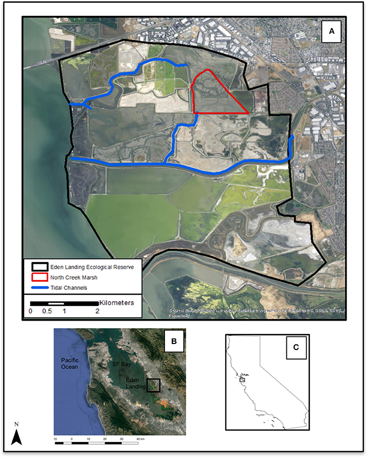
Figure 1. (A) Eden Landing Ecological Reserve (CA Dept. Fish and Wildlife), Hayward, California, USA. (B) South San Francisco Bay, Eden Landing Ecological Reserve outlined (C) California state outline. Aerial images reproduced with permission from ^©Google, 2017.

Salinity Data Analysis

We determined mean annual salinity for each rain year (October–September) between 2009 and 2015 using Station 30 from the USGS SF Bay water quality archive (Cloern and Schraga, 2016). To explore potential differences between tidal heights, we determined mean higher high water (MHHW) and monthly maximum tide from the NOAA Redwood City Tide Gauge, the closest tide station with continuous data over the study period (https://tidesandcurrents.noaa.gov/). For salinity and MHHW, we subset the data for rain years 2009–2011 and 2012–2015 to correspond to the dates of our imagery and California's historic drought. To determine differences between the two periods, we performed a non-parametric Kruskal–Wallis test for salinity, MHHW and monthly maximum tide. To determine directional trends in salinity during the two periods, we used non-parametric generalized additive models to analyze salinity levels over time using the gam package in R (Hastie, 2013). Non-parametric tests were used due to non-normality of salinity data.

Remote Sensing Data and Image Pre-processing

For 2009 and 2011, we obtained 0.8 m pan sharpened IKONOS imagery of the South Bay Salt Pond Restoration Project from the San Francisco Estuary Institute (^©Digital Globe Inc., 2011). For 2015, we obtained 0.5 m WorldView-2 imagery (^©Digital Globe Inc., 2015). Each set of imagery contained four spectral bands: red, green, blue, and near-infrared (NIR). To ensure phenological continuity between collection dates, all images were collected near peak biomass (June 23 2009, July 7 2011, and June 21 2015) at low tide to ensure maximum visibility of vegetation. The timing of collection is essential because tidal water frequently covers landscape features, such as vegetation patches, essential to change detection. To double check that intermediate years at our site did not exhibit anomalous vegetation growth that is not accounted for in our analysis, we reviewed Google Earth imagery (^©Google, 2017) for all available dates between June 2009 and June 2015. We did not find evidence of anomalous change or loss in the periods between our high resolution images.

To prepare the images for analysis, we re-projected the 2009 image from the GCS 1984 datum to the NAD 1983 datum to match the 2011 and 2015 images. We down-sampled all images to 0.8 m pixel resolution to match the lowest resolution images. We then geocorrected all images, resulting in an offset of 0.5 pixel maximum. Images were imported into eCognition (^©Trimble Inc.) software to perform OBIA. To allow for the most effective interpretation of vegetation patches, bands 4, 3, and 2 were visualized as RGB, respectively, and the Histogram Equalization stretch was applied across the image.

Object-Based Image Classification

Object-based analyses were performed in eCognition Developer software version 8.8 (^©Trimble Inc.). As a first step, we generated primitive image objects as spatial units for wetland classification using the Multiscale Resolution Segmentation (MRS) tool which requires the parameters of scale, shape and compactness to control object size and heterogeneity. For all images, we used the red, green, blue, and infrared bands to classify imagery. To determine their values for our objectives, we worked through a series of scale parameter values in increments of 5, and both shape and compactness parameters in increments of 0.1. We assessed each combination of settings by trial and error to determine which combination of parameters best matched the visual distribution of vegetation at the site. Notably, due to the differences in the original resolution of image datasets, we had to individually adjust their MRS parameters to obtain primitive objects of comparable size. For the 2011 image, using a scale of 10 resulted in unrealistically small objects. Using scales of 40 and above did not capture enough of the surface variation, and after comparison of incremental steps, we determined that a scale of 30 most effectively captured the vegetation patterning on the marsh surface. We selected a scale of 25 for the 2015 image and a scale of 6 for the 2009 image. For all images, shape was given low weight (0.1) in the final classification, as shapes in wetland vegetation are highly dependent on patch size and do not conform to regular patterns across the marsh surface (Moffett and Gorelick, 2013). Compactness was given a medium weight (0.5). For all images, the four bands were given equal weight.

Following the segmentation process, we manually identified at least 50 training samples for each of the three main categories: Water/Channels, Mudflat, and Vegetation. Vegetation is included as a simple category since the majority of vegetation at the site consists of Salicornia pacifica, an early-colonizing marsh dominant (Krause, 2016). Jaumea carnosa (Fleshy Jaumea), Frankenia salina (Alkali Heath), the annual Salicornia europaea (common glasswort), G. stricta (marsh gumplant), and S. foliosa (California cordgrass) are present in lower densities due to natural recruitment (Krause, 2016) and planting (Hammond, 2016), but our imagery did not allow for differentiation between species. Samples were selected by examining the imagery and cross-referencing these observations with checks of Google Earth (^©2015 Google) imagery to verify vegetation patterns. This information was combined with expert knowledge on vegetation patterns from field visits conducted between 2013 and 2015. Once samples were selected, images were classified by including a supervised nearest neighbor process algorithm with the mean brightness, mean NIR and standard deviation of the red band selected as class-discriminating features. We initially included the Normalized Difference Vegetation Index (NDVI), which uses the red and infrared bands to detect green vegetation, as a classification parameter. However, this led to spurious identification of algae as vegetation, and misclassified vegetated areas with apparent mudfilms as mudflat, so we elected not to include it in the final process decision tree. Following sample selection and implementation of the nearest neighbor algorithm, images from all years were separately classified into the three categories using the classification algorithm in eCognition. Once images from each year had been classified, the resulting classifications were imported into ENVI to perform change detection analysis via simple spatial overlay. Images were masked to include only the marsh-plain area.

To perform accuracy assessment, we used the Random Points tool (Standard C Rand function) in ArcGIS v. 10.3 (Esri Inc.) to select between 54 and 87 points per category per year, excluding training samples, and visually identified cover categories. Samples that fell along object edges were excluded from the random point selection. Google Earth images (^©2015 Google) from each year were used to manually verify sample collection points. These points were imported as Regions of Interest (ROI) into ENVI v.5.2 (Harris Geospatial Inc.) software to perform accuracy analysis. The ROIs were used to populate the Confusion Matrix tool, which calculates standard accuracy metrics (overall accuracy, kappa, user's, and producer's accuracies for different classes) of a classified image based on verified samples.

Following classification, we analyzed vegetation patch dynamics. To determine the relationship between vegetation presence and channel structure, we digitized a vector of the major channels at the site, then created a distance raster using the Euclidean Distance tool in ArcGIS v. 10.3 (Esri Inc.). This tool calculates the distance from a specified feature and outputs a continuous raster with corresponding values. We generated 1,000 random points using the Random Points tool in ArcGis and extracted the vegetation layer from our classification for each year. Based on this data we used vegetation presence (1) and absence (0) to run a generalized linear model with a binomial distribution using the lme4 package in R (Bates et al., 2017). To determine changes in patch configuration across the three images, we ran patch statistics using FragStats v. 4 (McGarigal et al., 2015).

Results

Salinity and Tides

Our results show that salinity was significantly higher during California's historic drought, and the magnitude of mean annual vegetation change was 10.4 times slower during this period compared to the lower salinity period that preceded it (Figures 2, 3). Mean salinity was 25.64 ppt for 2009–2010, and 23.99 ppt for 2010–2011, with an overall mean of 24.82 ppt (CV = 0.198) between 2009 and 2011. Mean salinity was 26.08 ppt for 2011–2012, 28.18 ppt for 2012–2013, 30.12 ppt for 2013–2014, and 29.50 ppt for 2014–2015, with a mean salinity of 28.47 ppt (CV = 0.10) between 2011 and 2015 (Figure 5). Salinity was significantly different between these two periods (p < 0.001, χ² = 18.40). Salinity significantly decreased between 2009 and 2011 (p < 0.001, F = 18.69) and significantly increased between 2011 and 2015 (p < 0.001, F = 16.50). Neither MHHW (p = 0.354, χ² = 0.86) nor monthly maximum tide was significantly different between the two periods (p = 0.354, χ² = 43.87) (Figure 2).

FIGURE 2

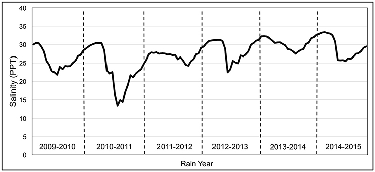
Figure 2. SF Bay Salinity, rain years 2009–2015. Data were taken from Station 30 of the bi-monthly USGS Water Quality Cruise (Cloern and Schraga, 2016).

FIGURE 3

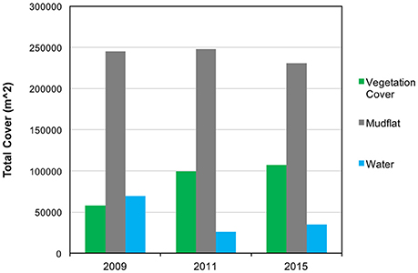
Figure 3. Cover type change. Mudflat was the dominant cover type across all 3 years. Vegetation increased at a rate of 20,580 m²/year between 2009 and 2011, and 1,979 m²/year between 2011 and 2015.

Remote Sensing Classification Accuracy

We obtained high classification accuracy for each of our cover categories in each year. For 2009, we obtained an overall accuracy of 92.42% and a Kappa Coefficient of 0.88. For 2011, we obtained an overall accuracy of 95.02% and a Kappa Coefficient of 0.92. For 2015, we obtained an overall accuracy of 96.83% and a Kappa Coefficient of 0.95. The lower overall accuracy in the 2009 image was due to over-classification of water on the marsh surface (Table 1). Vegetation, the focal target of post-restoration monitoring, was consistently classified with high user's and producer's accuracy exceeding 92% at all times (Table 1). It was most commonly misclassified with water in 2009 and 2015 and mudflat in 2011. Some of the overall classification error also occurred due to misclassification of water and mudflats that did not correspond to vegetation per se and thus was of lower concern for our objectives.

TABLE 1

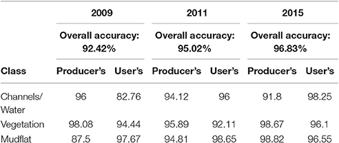
Table 1. Accuracy assessment for each cover category for 2009, 2011, and 2015.

Changes in Vegetation Cover and Distribution

Total vegetation cover increased from 58,154 m² of the study area to 99,315 m² from 2009 to 2011, an increase of 70.77% at a mean rate of 20,580 m²/year. In contrast, vegetation cover increased from 99,315 m² in 2011 to 107,232 m² in 2015, a 7.97% change from the 2011 cover at a mean rate of 1,979 m²/year (Figures 3, 4). For all years, vegetation presence was significantly related to distance from channel, with areas closer to channel more likely to support vegetation, but the magnitude of the effect was notably larger in the 2015 image (2009: p < 0.001, z = −3.49; 2011: p = 0.002, z = −2.98; 2015: p < 0.001, z = −6.33). In the 2011 image, we observed some vegetation colonization of interior mudflat areas that did not persist in the 2015 image (Figures 4, 5). The overall number of patches decreased from 2009 (394 patches) to 2011 (282 patches) and increased in 2015 (473 patches). Mean patch area was the largest in 2011 (352 m²), intermediate in 2015 (226 m²), and smallest in 2009 (147 m²; Table 2).

FIGURE 4

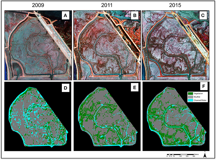
Figure 4. Change over time at North Creek Marsh. (A–C) False color imagery for 2009, 2011, and 2015. (D–F) Classifications of cover types for 2009, 2011, and 2015. Aerial images reproduced with permission from ^©DigitalGlobe, 2017.

FIGURE 5

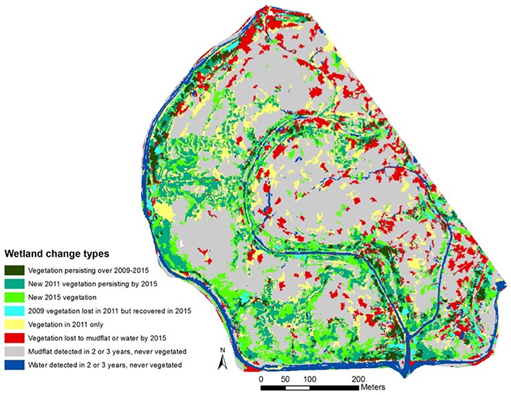
Figure 5. Change detection image at North Creek Marsh, 2009–2011. Vegetation is largely concentrated along channel edges. Interior areas are largely persistent mudflat over the entire study period. Some interior areas away from channels contain vegetation in the 2011 classification only that is subsequently lost in 2015.

TABLE 2

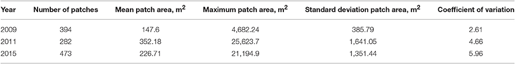
Table 2. Patch statistics for 2009, 2011, and 2015.

Among non-vegetated surfaces, mudflats were the most prevalent cover class across all years, declining slightly in 2015, with total cover of 245,413 m² in 2009, 247,685 m² in 2011, and 230,752 m² in 2015. Since the amount of water in aerial images is highly dependent on the timing of image, tidal phase, and other stochastic factors, changes in water coverage should be interpreted with caution. In our images, water accounted for 69,764 m² in 2009, 26,188 m² in 2011, and 34,787 m² in 2015 (Figures 3, 4).

Discussion

Post-restoration Vegetation Dynamics in Tidal Wetlands

Our results demonstrate that drought may impact vegetation change rates in Mediterranean-type tidal wetland restoration projects, leading to non-linear recovery patterns. At North Creek Marsh, vegetation cover increased from 2009 to 2011 and from 2011 to 2015, but the mean annual rate of change during the first period, when Bay salinity was lower, was more than 10 times as rapid as change during the second period, when historic drought conditions elevated salinity levels in the Bay. By employing remotely sensed imagery to study this progression, we were able to scale up from previous field efforts that demonstrated the effect of lowered salinity on plant productivity (Zedler, 1983; Schile et al., 2011; Woo and Takekawa, 2012), and restoration trajectories (Chapple et al., 2017). Previous work from Southern California documented increased rates of S. foliosa establishment in response to increased sedimentation rates brought on by El Nino events (Ward et al., 2003) and increased Spartina biomass and structure in response to lowered salinity brought on by El Nino events (Zedler, 1983; Zedler et al., 1986). Our results show that freshwater availability may also influence the rate of vegetation expansion in recently restored wetlands dominated by S. pacifica. These larger-scale observations are supported by experimental results that demonstrate that increased salinity levels reduced S. pacifica biomass production (Schile et al., 2011; Woo and Takekawa, 2012). In contrast to our site, a similar restoration project in a more freshwater marsh without a notable drought period reached 90% vegetated over a 10 year period, with no evidence of slowing pace after initial gains (Tuxen et al., 2008). This indicates that restoration projects in higher salinity regions may exhibit more variable, less linear trajectories due to interannual variability in salinity. While increased inundation during periods of higher rainfall could be another factor influencing vegetation change, we found no significant difference in MHHW or monthly maximum tide between the two periods.

Our results also demonstrate that channel structure is a key determinant of where vegetation establishes, and may be even more important during periods of elevated salinity. Vegetation was significantly associated with channel proximity for all years, but between 2011 and 2015, the strength of the interaction between vegetation presence and channel proximity more than doubled. We also visually observed establishment of new vegetation patches in interior marsh areas in 2011 (Figure 4), but these patches did not persist in 2015. Channels drive the restoration process by improving drainage across the marsh surface and lowering salinity (Sanderson et al., 2000; Williams and Orr, 2002; Wallace et al., 2005; O'Brien and Zedler, 2006). Biomass production of S. pacifica is significantly influenced by elevated salinity in in poorly drained areas, but has no effect in well-drained areas adjacent to channels (Schile et al., 2011). Our results indicate that salinity levels likely interact with the channel structure at the site, allowing vegetation to persist and expand in areas adjacent to channels but precluding development in poorly drained interior areas. Under projected climate change scenarios, increased prevalence of drought is likely to reduce snowpack and increase salinity (Callaway et al., 2007). This may slow the overall rate of vegetation change and increase the importance of channel structure in the restoration process.

The Potential of OBIA for Wetland Monitoring and Future Research Needs

Our results also show how OBIA can be used to overcome some of the challenges with high resolution data to map vegetation change over time in developing tidal wetlands. The dynamic nature of tidal processes mean that images are often different from each other based on how mud and water appear in the image, which can present problems for comparing images from different years (Dronova, 2015; Campbell et al., 2017). Furthermore, local noise and spectral variation, especially pronounced at higher spatial resolution, pose considerable challenges for delineating wetland cover type patches as semantic entities (Moffett and Gorelick, 2013), particularly at early post-restoration stages with higher spatial heterogeneity (Tuxen and Kelly, 2008; Tuxen et al., 2008; Kelly et al., 2011). By using object-based methods, we were able to create realistic objects for our cover types that produced high levels of accuracy, allowing for comparison between years at high spatial resolution. While NDVI has historically been employed as a means of detecting vegetation, we found that classification parameters that relied too heavily on NDVI led to classification of areas with green algae on the mudflat surface as vegetation. By also taking into account spatial parameters, our object-based approach minimized spurious mapping of vegetation that may occur when using pixel-based change methods. Our results highlight the distinct benefit of using OBIA in assessing early stages of restoration project development to capture fine scale change and to streamline semi-automated vegetation detection despite some degree of required specificity of methods and parameters at individual dates. Although OBIA benefits in wetland analyses have long been recognized (Tuxen and Kelly, 2008; Dronova, 2015), this methodology is still under-utilized in the context of restoration monitoring (Klemas 2013) and offers powerful opportunities for cost-effective, spatially comprehensive, and repeated characterizations of vegetation development and landscape structure.

Notably, different algorithm parameters were needed for each image to produce images with the highest accuracy. We were able to attain a high level of accuracy across all three images, but accuracy was slightly lower in the in the 2009 imagery, when algae and surface water led to more confusion between classes, highlighting the importance of date-specific conditions on wetland surface analysis in tidal systems. Distributions of water and mud across the landscape were mapped differently in different years, due to different tidal heights at the time of collection and evolving morphology of landscape topography that likely led to retention of water in different areas across the years. We suggest that changes between mudflat and water should be interpreted with caution, since they are highly temporally variable and sensitive to when imagery was collected. While vegetation increased overall, there were also notable areas of localized vegetation loss (particularly in areas farther from channels), which indicates that the site is still evolving. We expect that efforts to monitor multiple restoration sites will likely need to create separate classifications for each site to minimize the impact of unique surface conditions at a given tidal stage and surface variability on classification effectiveness.

Limitations and Future Directions

In addition to the effects of wet years and drought, the trends we observed are likely influenced by a combination of other factors. In the commonly accepted models of tidal wetland development, sedimentation rates are expected to slow as the marsh plain reaches equilibrium with tidal inundation (Morris et al., 2002; Williams and Orr, 2002; D'Alpaos et al., 2012; Schile et al., 2014), which could explain the observed decrease in the rate of vegetation expansion we observed. However, sedimentation data collected at the site shows that annual sedimentation rates between the breach date in 2006 and 2013 were marginally slower (1.21 cm/year) than between 2013 and 2016 (1.33 cm/year), when drought conditions persisted (Krause, 2016). This indicates that the decreased rate of vegetation expansion is not due to decreased rates of sedimentation. Further, between 2012 and 2015, S. foliosa was planted across the study site (Hammond, 2016). Since these plantings were largely adjacent to areas of existing vegetation, they may have contributed to the expansion we observed, which means that rates of natural expansion during the drought years may have been even lower than our results indicate. Lastly, our analysis of tidal height data shows that differences in tidal inundation did not differ between the wet and dry periods.

The inability to detect species-level trends is an important limitation of our study. In addition to the S. foliosa plantings, the tidal wetland sub-dominant species F. salina (Alkali Heath) and J. carnosa (Fleshy Jaumea) were also present at the site in very low densities (Krause, 2016). Work from older restoration and reference sites in the north SF Bay indicates that Bay salinity can also influence the dynamics of sub-dominant species (Chapple et al., 2017), which may be a promising direction for future studies in these areas. However, S. pacifica is the dominant species in the early stages of restoration in the area, and is responsible for the majority of vegetation cover. One of the major implications of rates of vegetation change is the ability of developing restoration projects to keep pace with sea level rise (Goals Project, 2015), so for the purposes of our study understanding overall rates of vegetation change is appropriate. Advancing this OBIA-based monitoring framework to develop a capacity to detect species-level transitions in the future is an important research need that could benefit from the advances in high-resolution hyperspectral platforms (Santos et al., 2011; Lucieer et al., 2014).

Implications for Restoration and Adaptive Management

Our results demonstrate that considering non-linear post-restoration site development trajectories that are dependent on weather may be crucial for structuring adaptive management decisions in variable climates. A detailed understanding of how weather interacts with site geomorphology to influence outcomes is important for planning effective restoration efforts (Holmgren and Scheffer, 2001; Vaughn and Young, 2010; Sitters et al., 2012; Chapple et al., 2017). Importantly, slower progress of vegetation is not entirely negative, as the intermediate habitat mosaic of vegetation, mudflat, and water provides habitat for a number of avian species (Moss, 2015). However, given that the rapid re-vegetation of tidal wetland restoration projects is considered to be one of the best means of allowing developing sites to keep pace with sea-level rise (Goals Project, 2015), understanding the role of weather in determining these rates will be essential for managing projects that are resilient to climate change.

Developing reproducible remote sensing techniques is a promising, potentially cost effective means of monitoring change in these projects over time. Future efforts should explore change over multiple sites to discern how generalized these weather-dependent trends are and how transferable image classification settings are between sites. Sampling restoration sites across a range of salinity levels in the SF Bay would allow for an exploration of how the spatial context of sites might influence their temporal development. Since field sampling is limited by time, scale, funding, and spatial resolution, remotely sensed products hold high promise for addressing these issues.

From a restoration management perspective, our findings supported other work demonstrating that channel edges are hotspots of vegetation development (Sanderson et al., 2000; Wallace et al., 2005; O'Brien and Zedler, 2006). Attempts to add diversity into developing marshes should focus on these areas, a practice which is already in place in the SF Bay (Hammond, 2016). Since we show that interior mudflat areas away from channels may be slow to develop vegetation, proactive manipulation of elevation in these areas prior to restoring tidal access may be one way to speed vegetation development. Further, efforts to actively manipulate channel structure may also help speed the development of vegetation establishment. These actions are likely to be more necessary in areas where salinity levels are currently higher, but may become necessary across a range of sites as climate change shifts salinity distributions in the SF Bay (Callaway et al., 2007). Proactive geomorphic intervention is likely to make these projects more resilient to the impacts of sea level rise.

Author Contributions

DC and ID conceived of the research. DC analyzed the data. DC and ID wrote and revised the manuscript.

Funding

DC's work on the project was supported by the NSF GRFP program (DGE 1106400) and UC Berkeley's Sponsored Projects for Undergraduate Research Program.

Conflict of Interest Statement

The authors declare that the research was conducted in the absence of any commercial or financial relationships that could be construed as a potential conflict of interest.

Acknowledgments

Thanks to Adina Merenlender, Katie Suding, Maggi Kelly, Laurel Larsen, John Krause, John Bourgeois, Kristin Byrd, Brian Fulfrost, Micah Levi, Manda Au, and Christian Tettlebach. Image registration was done by Sean Hogan at the UCANR Informatics and GIS Program. CA Department of Fish and Wildlife provided site access and the San Francisco Estuary Institute provided imagery for 2009 and 2011. Two reviewers provided feedback that greatly improved the manuscript. Appropriate permissions have been obtained from copyright holders for all reproduced imagery.

References

Asner, G. P., Brodrick, P. G., Anderson, C. B., Vaughn, N., Knapp, D. E., and Martin, R. E. (2016). Progressive forest canopy water loss during the 2012–2015 California drought. Proc. Natl. Acad. Sci. U.S.A. 113, E249–E255. doi: 10.1073/pnas.1523397113

PubMed Abstract | CrossRef Full Text | Google Scholar

Bates, D., Maechler, M., Bolker, B., and Walker, S. (2017). lme4: Linear Mixed-Effects Models Using EIGEN and S4. Available online at: http://CRAN.R-project.org/package=lme4

Berg, N., and Hall, A. (2017). Anthropogenic warming impacts on California snowpack during drought. Geophys. Res. Lett. 44, 2511–2518. doi: 10.1002/2016GL072104

CrossRef Full Text | Google Scholar

Bernhardt, E. S., Sudduth, E. B., Palmer, M. A., Allan, J. D., Meyer, J. L., Alexander, G., et al. (2007). Restoring rivers one reach at a time: results from a survey of US river restoration practitioners. Restor. Ecol. 15, 482–493. doi: 10.1111/j.1526-100X.2007.00244.x

CrossRef Full Text | Google Scholar

Blaschke, T., and Hay, G. J. (2001). Object-oriented image analysis and scale-space: theory and methods for modeling and evaluating multiscale landscape structure. Int. Arch. Photogramm. Remote Sens. 34, 22–29.

Google Scholar

Blaschke, T., Lang, S., Lorup, E., Strobl, J., and Zeil, P. (2000). Object-oriented image processing in an integrated GIS/remote sensing environment and perspectives for environmental applications. Environ. Informat. Plann. Politic. Public 2, 555–570.

Google Scholar

Brand, L. A., Smith, L. M., Takekawa, J. Y., Athearn, N. D., Taylor, K., Shellenbarger, G. G., et al. (2012). Trajectory of early tidal marsh restoration: elevation, sedimentation and colonization of breached salt ponds in the northern San Francisco Bay. Ecol. Eng. 42, 19–29. doi: 10.1016/j.ecoleng.2012.01.012

CrossRef Full Text | Google Scholar

Brew, D. S., and Williams, P. B. (2010). Predicting the impact of large-scale tidal wetland restoration on morphodynamics and habitat evolution in south San Francisco Bay, California. J. Coastal Res. 26, 912–924. doi: 10.2112/08-1174.1

CrossRef Full Text | Google Scholar

Callaway, J. C., Thomas Parker, V., Vasey, M. C., and Schile, L. M. (2007). Emerging issues for the restoration of tidal marsh ecosystems in the context of predicted climate change. Madroño 54, 234–248. doi: 10.3120/0024-9637(2007)54[234:EIFTRO]2.0.CO;2

CrossRef Full Text | Google Scholar

Callaway, R. M., and Sabraw, C. S. (1994). Effects of variable precipitation on the structure and diversity of a California salt marsh community. J. Veget. Sci. 5, 433–438. doi: 10.2307/3235867

CrossRef Full Text | Google Scholar

Campbell, A., Wang, Y., Christiano, M., and Stevens, S. (2017). Salt Marsh Monitoring in Jamaica Bay, New York from 2003 to 2013: a decade of change from restoration to hurricane sandy. Remote Sens. 9:131. doi: 10.3390/rs9020131

CrossRef Full Text | Google Scholar

Chapple, D. E., Faber, P., Suding, K. N., and Merenlender, A. M. (2017). Climate variability structures plant community dynamics in mediterranean restored and reference tidal wetlands. Water 9:209. doi: 10.3390/w9030209

CrossRef Full Text | Google Scholar

Cloern, J. E., and Schraga, T. S. (2016). USGS Measurements of Water Quality in San Francisco Bay (CA), 1969-2015, Version 2. U.S. Geological Survey Release. U.S. Geological Survey.

Conchedda, G., Durieux, L., and Mayaux, P. (2008). An object-based method for mapping and change analysis in mangrove ecosystems. Isprs J. Photogramm. Remote Sens. 63, 578–589. doi: 10.1016/j.isprsjprs.2008.04.002

CrossRef Full Text | Google Scholar

Copeland, S. M., Harrison, S. P., Latimer, A. M., Damschen, E. I., Eskelinen, A. M., Fernandez-Going, B., et al. (2016). Ecological effects of extreme drought on Californian herbaceous plant communities. Ecol. Monogr. 86, 295–311. doi: 10.1002/ecm.1218

CrossRef Full Text | Google Scholar

D'Alpaos, A., Da Lio, C., and Marani, M. (2012). Biogeomorphology of tidal landforms: physical and biological processes shaping the tidal landscape. Ecohydrology 5, 550–562. doi: 10.1002/eco.279

CrossRef Full Text | Google Scholar

Dettinger, M. D., and Cayan, D. R. (2003). Interseasonal covariability of Sierra Nevada streamflow and San Francisco Bay salinity. J. Hydrol. 277, 164–181. doi: 10.1016/S0022-1694(03)00078-7

CrossRef Full Text | Google Scholar

Diggory, Z. E., and Parker, V. T. (2011). Seed supply and revegetation dynamics at restored tidal marshes, Napa River, California. Restor. Ecol. 19, 121–130. doi: 10.1111/j.1526-100X.2009.00636.x

CrossRef Full Text | Google Scholar

Dronova, I. (2015). Object-based image analysis in wetland research: a review. Remote Sens. 7:6380–6413. doi: 10.3390/rs70506380

CrossRef Full Text | Google Scholar

Erwin, K. L. (2009). Wetlands and global climate change: the role of wetland restoration in a changing world. Wetlands Ecol. Manag. 17, 71. doi: 10.1007/s11273-008-9119-1

CrossRef Full Text | Google Scholar

Fulfrost, B., Thomson, D., Archibald, G., Loy, C., and Fourt, W. (2012). Habitat Evolution Monitoring Program: South Bay Salt Pond Restoration Project, Final Report (2009-2011). Prepared for California Coastal Conservancy.

Gaertner, P., Foerster, M., Kurban, A., and Kleinschmit, B. (2014). Object based change detection of Central Asian Tugai vegetation with very high spatial resolution satellite imagery. Int. J. Appl. Earth Observ. Geoinform. 31, 110–121. doi: 10.1016/j.jag.2014.03.004

CrossRef Full Text | Google Scholar

Goals Project (2015). The Baylands and Climate Change: What We Can Do. Baylands Ecosystem Habitat Goals Science Update 2015. San Francisco Bay Area Wetlands Ecosystem Goals Project, California State Coastal Conservancy.

Hammond, J. (2016). San Francisco Estuary Invasive Spartina Project Revegetation Program 2014–2015 Installation Report and 2015-2016 Revegetation Plan. Oakland, CA: California State Coastal Conservancy.

Hastie, T. (2013). gam: Generalized Additive Models, R Package, Version 0.98. Available online at: www.r-project.com

Holmgren, M., and Scheffer, M. (2001). El Niño as a window of opportunity for the restoration of degraded arid ecosystems. Ecosystems 4, 151–159. doi: 10.1007/s100210000065

CrossRef Full Text | Google Scholar

Holmgren, M., Stapp, P., Dickman, C. R., Gracia, C., Graham, S., Gutiérrez, J. R., et al. (2006). Extreme climatic events shape arid and semiarid ecosystems. Front. Ecol. Environ. 4, 87–95. doi: 10.1890/1540-9295(2006)004[0087:ECESAA]2.0.CO;2

CrossRef Full Text | Google Scholar

Kelly, M., Tuxen, K. A., and Stralberg, D. (2011). Mapping changes to vegetation pattern in a restoring wetland: finding pattern metrics that are consistent across spatial scale and time. Ecol. Indic. 11, 263–273. doi: 10.1016/j.ecolind.2010.05.003

CrossRef Full Text | Google Scholar

Klemas, V. (2013). Using remote sensing to select and monitor wetland restoration sites: an overview. J. Coast. Res. 29, 958–970. doi: 10.2112/JCOASTRES-D-12-00170.1

CrossRef Full Text | Google Scholar

Kondolf, G. M., Anderson, S., Lave, R., Pagano, L., Merenlender, A., and Bernhardt, E. S. (2007). Two decades of river restoration in California: what can we learn? Restor. Ecol. 15, 516–523. doi: 10.1111/j.1526-100X.2007.00247.x

CrossRef Full Text | Google Scholar

Krause, J. (2016). CDFW Marsh Monitoring Field Form: Vegetation and Sediment. Sacramento, CA: California Department of Fish and Wildlife.

Lucieer, A., Malenovsky, Z., Veness, T., and Wallace, L. (2014). HyperUAS—imaging spectroscopy from a multirotor unmanned aircraft system. J. Field Robot. 31, 571–590. doi: 10.1002/rob.21508

CrossRef Full Text | Google Scholar

Malamud-Roam, F., and Ingram, B. L. (2004). Late Holocene δ 13 C and pollen records of paleosalinity from tidal marshes in the San Francisco Bay estuary, California. Q. Res. 62, 134–145. doi: 10.1016/j.yqres.2004.02.011

CrossRef Full Text | Google Scholar

McGarigal, K., Cushman, S. A., Neel, M. C., and Ene, E. (2015). FRAGSTATS: spatial Pattern Analysis Program for Categorical Maps. Computer Software Program Produced by the Authors at the University of Massachusetts, Amherst. Available online at: http://www.umass.edu/landeco/research/fragstats/fragstats.html

Moffett, K. B., and Gorelick, S. M. (2013). Distinguishing wetland vegetation and channel features with object-based image segmentation. Int. J. Remote Sens. 34, 1332–1354. doi: 10.1080/01431161.2012.718463

CrossRef Full Text | Google Scholar

Moffett, K. B., and Gorelick, S. M. (2016). Alternative stable states of tidal marsh vegetation patterns and channel complexity. Ecohydrology 9, 1639–1662. doi: 10.1002/eco.1755

CrossRef Full Text | Google Scholar

Morris, J. T., Sundareshwar, P. V., Nietch, C. T., Kjerfve, B., and Cahoon, D. R. (2002). Responses of coastal wetlands to rising sea level. Ecology 83, 2869–2877. doi: 10.1890/0012-9658(2002)083[2869:ROCWTR]2.0.CO;2

CrossRef Full Text | Google Scholar

Moss, B. (2015). Mammals, freshwater reference states, and the mitigation of climate change. Freshwater Biol. 60, 1964–1976. doi: 10.1111/fwb.12614

CrossRef Full Text | Google Scholar

O'Brien, E. L., and Zedler, J. B. (2006). Accelerating the restoration of vegetation in a southern California salt marsh. Wetlands Ecol. Manag. 14, 269–286. doi: 10.1007/s11273-005-1480-8

CrossRef Full Text | Google Scholar

Pachauri, R. K., Allen, M. R., Barros, V. R., Broome, J., Cramer, W., Christ, R., et al. (2014). Climate Change 2014: Synthesis Report. Contribution of Working Groups I, II and III to the fifth Assessment Report of the Intergovernmental Panel on Climate Change. Geneva: IPCC. Available online at: http://epic.awi.de/37530/ (Accessed October 18, 2016).

Google Scholar

Peters, D. P., Pielke, R. A., Bestelmeyer, B. T., Allen, C. D., Munson-McGee, S., and Havstad, K. M. (2004). Cross-scale interactions, nonlinearities, and forecasting catastrophic events. Proc. Natl. Acad. Sci. U.S.A. 101, 15130–15135. doi: 10.1073/pnas.0403822101

PubMed Abstract | CrossRef Full Text | Google Scholar

Philip Williams & Associates, Ltd., and Faber, P. M. (2004). Design Guidelines for Tidal Wetland Restoration in San Francisco Bay (San Francisco, CA: The Bay Institue).

Robeson, S. M. (2015). Revisiting the recent California drought as an extreme value. Geophys. Res. Lett. 42, 6771–6779. doi: 10.1002/2015GL064593

CrossRef Full Text | Google Scholar

Sanderson, E. W., Ustin, S. L., and Foin, T. C. (2000). The influence of tidal channels on the distribution of salt marsh plant species in Petaluma Marsh, CA, USA. Plant Ecol. 146, 29–41. doi: 10.1023/A:1009882110988

CrossRef Full Text | Google Scholar

Santos, M. J., Anderson, L. W., and Ustin, S. L. (2011). Effects of invasive species on plant communities: an example using submersed aquatic plants at the regional scale. Biol. Invasions 13, 443–457. doi: 10.1007/s10530-010-9840-6

CrossRef Full Text | Google Scholar

Scheffer, M., Bascompte, J., Brock, W. A., Brovkin, V., Carpenter, S. R., Dakos, V., et al. (2009). Early-warning signals for critical transitions. Nature 461, 53–59. doi: 10.1038/nature08227

PubMed Abstract | CrossRef Full Text | Google Scholar

Schiewe, J., Tufte, L., and Ehlers, M. (2001). Potential and problems of multi-scale segmentation methods in remote sensing. GeoBIT/GIS 6, 34–39.

Schile, L. M., Callaway, J. C., Morris, J. T., Stralberg, D., Parker, V. T., and Kelly, M. (2014). Modeling tidal marsh distribution with sea-level rise: evaluating the role of vegetation, sediment, and upland habitat in marsh resiliency. PLoS ONE 9:e88760. doi: 10.1371/journal.pone.0088760

PubMed Abstract | CrossRef Full Text | Google Scholar

Schile, L. M., Callaway, J. C., Parker, V. T., and Vasey, M. C. (2011). Salinity and inundation influence productivity of the halophytic Plant Sarcocornia pacifica. Wetlands 31, 1165–1174. doi: 10.1007/s13157-011-0227-y

CrossRef Full Text | Google Scholar

Sitters, J., Holmgren, M., Stoorvogel, J. J., and López, B. C. (2012). Rainfall-tuned management facilitates dry forest recovery. Restor. Ecol. 20, 33–42. doi: 10.1111/j.1526-100X.2010.00761.x

CrossRef Full Text | Google Scholar

Son, N.-T., Chen, C.-F., Chang, N.-B., Chen, C.-R., Chang, L.-Y., and Thanh, B.-X. (2015). Mangrove mapping and change detection in Ca Mau Peninsula, Vietnam, using landsat data and object-based image analysis. IEEE J. Select. Top. Appl. Earth Observ. Remote Sens. 8, 503–510. doi: 10.1109/JSTARS.2014.2360691

CrossRef Full Text | Google Scholar

Spencer, T., Schuerch, M., Nicholls, R. J., Hinkel, J., Lincke, D., Vafeidis, A. T., et al. (2016). Global coastal wetland change under sea-level rise and related stresses: the DIVA wetland change model. Glob. Planet. Change 139, 15–30. doi: 10.1016/j.gloplacha.2015.12.018

CrossRef Full Text | Google Scholar

Stanford, B. R. M., Grossinger, J., Beagle, R. A., Askevold, R. A., Leidy, E. E., et al. (2013). Alameda Creek Watershed Historical Ecology Study. Richmond, CA: San Francisco Estuary Institute.

Suding, K. N., Gross, K. L., and Houseman, G. R. (2004). Alternative states and positive feedbacks in restoration ecology. Trends Ecol. Evol. 19, 46–53. doi: 10.1016/j.tree.2003.10.005

PubMed Abstract | CrossRef Full Text | Google Scholar

Trulio, L., Clark, D., Richie, S., and Hutzel, A. (2007). Adaptive Management Plan: Science Team Report for the South Bay Salt Pond Restoration Project. California Coastal Conservancy.

Tuxen, K. A., Schile, L. M., Kelly, M., and Siegel, S. W. (2008). Vegetation colonization in a restoring tidal marsh: a remote sensing approach. Restor. Ecol. 16, 313–323. doi: 10.1111/j.1526-100X.2007.00313.x

CrossRef Full Text | Google Scholar

Tuxen, K., and Kelly, M. (2008). “Multi-scale functional mapping of tidal marsh vegetation using object-based image analysis,” in Object-Based Image Analysis (Springer), 415–442. Available online at: http://link.springer.com/chapter/10.1007/978-3-540-77058-9_23 (accessed May 5, 2015).

Google Scholar

Tuxen, K., Schile, L., Stralberg, D., Siegel, S., Parker, T., Vasey, M., et al. (2011). Mapping changes in tidal wetland vegetation composition and pattern across a salinity gradient using high spatial resolution imagery. Wetlands Ecol. Manag. 19, 141–157. doi: 10.1007/s11273-010-9207-x

CrossRef Full Text | Google Scholar

Vaughn, K. J., and Young, T. P. (2010). Contingent conclusions: year of initiation influences ecological field experiments, but temporal replication is rare. Restor. Ecol. 18, 59–64. doi: 10.1111/j.1526-100X.2010.00714.x

CrossRef Full Text | Google Scholar

Wallace, K. J., Callaway, J. C., and Zedler, J. B. (2005). Evolution of tidal creek networks in a high sedimentation environment: a 5-year experiment at Tijuana Estuary, California. Estuar. Coasts 28, 795–811. doi: 10.1007/BF02696010

CrossRef Full Text | Google Scholar

Wang, L., Sousa, W. P., and Gong, P. (2004). Integration of object-based and pixel-based classification for mapping mangroves with IKONOS imagery. Int. J. Remote Sens. 25, 5655–5668. doi: 10.1080/014311602331291215

CrossRef Full Text | Google Scholar

Ward, K. M., Callaway, J. C., and Zedler, J. B. (2003). Episodic colonization of an intertidal mudflat by native cordgrass (Spartina foliosa) at Tijuana Estuary. Estuar. Coasts 26, 116–130. doi: 10.1007/BF02691699

CrossRef Full Text | Google Scholar

Watson, E. B. (2008). Marsh expansion at Calaveras Point Marsh, South San Francisco Bay, California. Estuar. Coast. Shelf Sci. 78, 593–602. doi: 10.1016/j.ecss.2008.02.008

CrossRef Full Text | Google Scholar

Williams, P. B., and Orr, M. K. (2002). Physical evolution of restored breached levee salt marshes in the San Francisco Bay estuary. Restor. Ecol. 10, 527–542. doi: 10.1046/j.1526-100X.2002.02031.x

CrossRef Full Text | Google Scholar

Williams, P., and Faber, P. (2001). Salt marsh restoration experience in San Francisco Bay. J. Coast. Res. 27, 203–211.

Google Scholar

Woo, I., and Takekawa, J. Y. (2012). Will inundation and salinity levels associated with projected sea level rise reduce the survival, growth, and reproductive capacity of Sarcocornia pacifica (pickleweed)? Aquat. Bot. 102, 8–14. doi: 10.1016/j.aquabot.2012.03.014

CrossRef Full Text | Google Scholar

Zedler, J. B. (1983). Freshwater impacts in normally hypersaline marshes. Estuaries 6, 346–355. doi: 10.2307/1351393

CrossRef Full Text | Google Scholar

Zedler, J. B. (2007). Success: an unclear, subjective descriptor of restoration outcomes. Ecol. Restor. 25, 162–168. doi: 10.3368/er.25.3.162

CrossRef Full Text | Google Scholar

Zedler, J. B., and Kercher, S. (2005). Wetland resources: status, trends, ecosystem services, and restorability. Annu. Rev. Environ. Res. 30, 39–74. doi: 10.1146/annurev.energy.30.050504.144248

CrossRef Full Text | Google Scholar

Zedler, J. B., Covin, J., Nordby, C., Williams, P., and Boland, J. (1986). Catastrophic events reveal the dynamic nature of salt-marsh vegetation in Southern California. Estuaries 9, 75–80. doi: 10.2307/1352195

CrossRef Full Text | Google Scholar

Zedler, J. B., Doherty, J. M., and Miller, N. A. (2012). Shifting restoration policy to address landscape change, novel ecosystems, and monitoring. Ecol. Soc. 17:36. doi: 10.5751/ES-05197-170436

CrossRef Full Text | Google Scholar