A Lab-On-Chip Phosphate Analyzer for Long-term In Situ Monitoring at Fixed Observatories: Optimization and Performance Evaluation in Estuarine and Oligotrophic Coastal Waters

Introduction

The availability of orthophosphate, the phosphorus species directly available to phytoplankton and autotrophic bacteria in natural waters, exerts a major influence on the productivity, phytoplankton species composition, and community structure of aquatic ecosystems. In inland waters, estuaries, and coastal water bodies, enhanced nutrient inputs resulting from human activities may result in algal growth exceeding the grazing capacity of organisms higher in the food chain, with cascading effects on water quality including hypoxia and the occurrence of toxin producing harmful algal blooms (National Research Council, 2000; Bricker et al., 2008). On a global scale, elucidating the upper ocean dynamics of phosphate (and other essential nutrient elements) is necessary to quantify particulate carbon export in the contemporary ocean and to develop robust numerical models which can then be used to elucidate the effect of a changing nutrient supply on the strength of the biological pump (Benitez-Nelson, 2000; Paytan and McLaughlin, 2007; Karl, 2014).

Much of our current understanding of the spatial patterns and temporal trends in phosphate concentrations stems from discrete sampling efforts performed at weekly to monthly intervals, followed by laboratory analysis using complex instrumentation. While this approach provides powerful insights into the cycling of phosphate in natural waters, such sampling rates are inadequate to characterize conditions during episodic and transient events, which can have a disproportionate impact on nutrient concentrations and significant ecological implications (Johnson et al., 2010). Without high-frequency data and a greater spatial coverage than can be afforded via discrete sampling, estimates of the nutrient load delivered into water bodies are fraught with uncertainties (Pellerin et al., 2014, 2016), and fine-scale 3D biogeochemical models cannot be properly validated to inform resource managers (Wild-Allen and Rayner, 2014). An improved understanding of biogeochemical variability is also needed to untangle natural vs. anthropogenic signals in time-series records. For these reasons, the development of in situ nutrient sensors with a dynamic quantification range suitable for high-frequency, long-term sampling in marine and inland waters is essential to improve our understanding of the fluxes and biogeochemical implications of nutrient distributions in aquatic ecosystems.

In the last 15 years, several research and commercial devices have been developed for in situ monitoring of phosphate in natural waters (Thouron et al., 2003; Jońca et al., 2013a; Legiret et al., 2013). The overwhelming majority of these devices are wet chemical analyzers (Jońca et al., 2013a), many of which operate using the molybdenum blue chemistry developed by Murphy and Riley (1962). Electrochemical reagentless sensors, which hold great promise for long-term unattended operations on fixed and mobile platforms, have recently been developed (Jońca et al., 2011, 2013b; Barus et al., 2016), but require further development and extensive field testing prior to use during field campaigns. By virtue of their robustness, low reagent and power consumption (1.8 W), ability to store waste onboard and to operate using established chemical protocols in a miniaturized manifold, microfluidic Lab-On-Chip sensors are well-suited to in situ monitoring in natural waters (Beaton et al., 2012; Nightingale et al., 2015; Yücel et al., 2015). In a companion paper, Clinton-Bailey et al. (2017) described a prototype phosphate LOC sensor and its application to in situ monitoring in a UK chalk stream. However, the performance of this LOC phosphate sensor in estuarine waters with a complex matrix and in oligotrophic coastal waters has not yet been rigorously investigated.

To encourage a more widespread use of in situ sensors by academics and resource managers, the challenge is not only to develop devices that are robust, compact, easy to operate and amenable to long term deployments (>month) but also to produce sensors that can meet or come close to the same stringent accuracy and precision criteria that are achieved in the laboratory. The latter criteria are rarely described in detail in the research literature, particularly over long deployment times. The overarching goal of this work is to report on the laboratory and field performance of a newly developed LOC phosphate analyzer, which is the next iteration of the sensor described in Clinton-Bailey et al. (2017). We start by describing the optimization of the most critical reaction parameters of the molybdenum blue method in order to obtain the highest possible analytical sensitivity and fast reaction kinetics, while minimizing the blank and Si interferences. The influence of temperature, sample salinity and Colored Dissolved Organic Matter (CDOM) on the accuracy of the phosphate determinations is then evaluated and an in situ correction scheme for sample salinity and sample color is proposed. We then perform a rigorous performance evaluation using data from a 56-days estuarine deployment in Southampton Water, as well as data from testing which occurred in 2016 as part of the Nutrient Sensor Challenge led by the Alliance for Coastal Technologies (https://www.act-us.info/nutrients-challenge/).

Materials and Methods

The phosphate sensor described in this work is a miniaturized batch analyzer, which automates the classic molybdenum blue batch method of Murphy and Riley (1962) using microfluidics. The molybdenum blue assay relies on the reaction of orthophosphates and acid-labile organic phosphorus compounds (collectively referred to as Soluble Reactive Phosphorus) with molybdate in an acidic solution to form molybdophosphoric acid. The molybdophosphoric acid is then reduced to phosphomolybdenum blue using ascorbic acid and its absorbance is quantified at 700 nm. The molybdenum blue assay implemented in this work has been optimized for in situ work using microfluidics (Clinton-Bailey et al., 2017).

Reagent Preparation

All reagents were prepared using Ultra High Purity (UHP) water (MilliQ >18.2 MΩ-cm, Millipore) and analytical grade salts (Sigma Aldrich). Acid-cleaned, low density polyethylene volumetric flasks and bottles were used to minimize contamination when preparing solutions. Stock solutions of potassium antimonyl tartrate (PAT; C₈H₄K₂O₁₂Sb₂·3H₂O, 4.5 mM), sodium hydroxide (NaOH, 1 M), and phosphate (KH₂PO₄, 1 mM) were prepared by dissolving the salts in UHP water. The phosphate and PAT stock solutions were stored in the dark at 4°C until use.

The molybdate reagent (R1, 500 mL) was prepared by dissolving 0.28 g of ammonium heptamolybdate tetrahydrate [(NH₄)₆Mo₇O₂₄.4H₂O], followed by 12 mL of 5 M H₂SO₄ and 6.25 mL of the PAT stock solution in 500 mL of UHP water. The final concentrations of the constituents in R1 were thus 0.45 mM ammonium molybdate, 120 mM H₂SO₄, and 0.06 mM PAT. A reducing solution (R2, 500 mL) was made by dissolving 5 g of L-ascorbic acid (C₆H₈O₆) and 0.05 g of polyvinylpyrrolidone (PVP) in 500 mL UHP water. A wash solution was prepared by diluting the stock NaOH to 0.01 M in 200 mL UHP water.

The working phosphate standards (500 mL each) were prepared by diluting the phosphate stock solution (1 mM) in low nutrient seawater (Ocean Scientific International Ltd., UK) previously acidified with 16 mM H₂SO₄ (pH ~ 1.7). The onboard blank solution (500 mL) consisted of acidified low nutrient seawater with no phosphate added. Acidifying the onboard blank and standards to pH < 2 was necessary to minimize adsorption of orthophosphate onto the walls of the storage bags. For deployments in brackish and estuarine waters, it is preferable to adjust the salinity of the onboard blank and standards using UHP water so that their salinity is close to the median salinity expected at the deployment location. However, it is also possible to prepare the blank and standards in acidified UHP water and correct for salinity induced refractive index differences between the samples and onboard standards in situ (see below).

All working solutions including waste were stored in flexible storage bags (FlexBoy, Sartorius-Stedim). The molybdate (R1), ascorbic acid (R2), blanks, and standards bags were covered with opaque tape to prevent photodegradation of the chemicals.

Microfluidic Sensor Description

The analyzer consisted of a circular, multi-layer microfluidic chip (Ø = 119 mm) manufactured from tinted poly(methyl methacrylate) (PMMA), a stepper motor mechanically linked to three 70 μL glass syringes, ten 300 series microinert solenoid valves (The Lee Company), and a custom electronics package for data logging and control (Figure 1). Details of the chip fabrication protocol, embedded electronics package, and communications will be reported elsewhere. The pumping system, valves, and electronics were mounted directly onto the microfluidic chip and were placed in an air-filled, watertight PVC housing (diameter: 12.5 cm, length: 19.5 cm). The chip formed the top end cap of the housing and was connected to the flexible fluid storage bags using 0.5 mm i.d. polytetrafluoroethylene (PTFE) tubing and ¼ 28″ connectors. The fluid storage bags (blank, reagents, standards, wash solution, and waste) were stored inside a second PVC tube (diameter: 15 cm, length: 45 cm) mounted above the sensor housing (Figure 1). The sensor sampling inlet, located at the bottom of the PVC tube hosting the reagents, was fitted with a 33 mm diameter, 0.45 μm pore size polyethersulfone syringe filter (SLPHP033RS, EMD Millipore, USA).

FIGURE 1

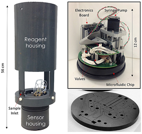
Figure 1. Pictures of the Lab-On-Chip phosphate sensor. (Left) A fully assembled sensor with reagent housing. (Top-right) A LOC sensor prior to placement in the watertight sensor housing. (Bottom) One of the PMMA layers of a phosphate Lab-On-Chip (Sensor 1) showing the micromilled microfluidic channels prior to sealing with the other layers of the microfluidic chip.

A schematic diagram of the microfluidic flow manifold is shown in Figure 2. The microfluidic channels, including the on-chip optical absorbance cells, were 150 μm wide and 300 μm deep (Figure 1). The fluidic manifold, included a reference cell (35 mm) and three measurement cells (long: 98 mm; medium: 35 mm; short: 2.5 mm) placed in series, downstream of the confluence point where the analyte solution and the two reagent streams are merged (Figure 2). Each cell was configured for absorbance detection using a 700 nm Light Emitting Diode (LED700-02AU, Roithner) and a measuring photodiode (TSLG257-LF, TAOS) placed at opposite ends of the cells (Ogilvie et al., 2010; Sieben et al., 2010; Floquet et al., 2011). In addition, monitoring photodiodes were positioned perpendicular to the LEDs of the reference, long and medium channels in order to monitor the intensity of the LEDs and, if needed, correct for drift (Figure 2).

FIGURE 2

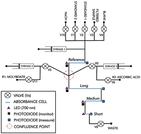
Figure 2. Schematic flow diagram of Sensor 2. This sensor is the latest version designed and manufactured at the National Oceanography Centre Southampton. Absorbance cells: Long: 98 mm; Medium: 35 mm; Short: 2.5 mm. The reference cell (35 mm, but not used in this work) may be used to determine the absorbance of the sample prior to addition of the reagents.

Analytical Protocol

A complete measurement cycle consisted of analyzing the blank solution, the filtered sample, and lastly the standards. After absorbance quantification of the most concentrated standard, the reference and measurement cells were flushed and filled with the 0.01 M NaOH wash solution to clean the channels until the next measurement cycle was triggered (Table S1). The analytical protocol involved injecting the analyte solution (blank, sample, or standards) and the two reagents into the measurement cells using a 1:1:1 ratio (v:v) via a confluence point located upstream of the cells (Figure 2). The flow was then stopped for 300 s while diffusive mixing and color development occurred within the measurement cells. The same analytical protocol and stopped flow times were applied to the blank, filtered sample, and standards.

To prevent carryover between blank, sample, and standards, the channels were first flushed with 210 μL of blank or standards and 350 μL of filtered sample (Table S1). The sample flushing volume was larger than that of the blank and standards to account for the volume of the sample inlet filter. After the last flush of blank and sample, the flow was stopped for 5 s in order to determine the absorbance of the sample without reagents added in each measurement cell (Table S1).

Data Processing

For each measurement cycle, the sample and standard(s) have an associated blank from which absorbance is calculated:

$Absorbance=-{\log }_{10}\left[\frac{V_S}{V_{BLK}}\times \frac{I_{BLK}}{I_S}\right]-OP{T}_{CORR}$

V_S and V_BLK are the mean voltages of the measuring photodiodes (located at the end of each cell) during the last 5 s of the stopped flow period of the sample or standard (V_S) and blank (V_BLK) measurements. I_BLK and I_S are the mean voltages of the monitoring photodiodes, which measure the LED outputs during the sample, standard and blank over the same period. The ratio of the blank and sample monitoring photodiodes voltages (i.e., I_BLK/I_S) is a scaling factor used to correct for the drift in the illumination intensity of the LEDs that may occur between the start (analysis of blank) and end (analysis of last standard) of the measurement sequence. This drift occurs due to the warming up of the LEDs during the measurement sequence and is not related to the reaction kinetics of the phosphomolybdenum blue complex formation. OPT_CORR (−log₁₀[V_S/V_BLK]) is the absorbance of the sample without reagents added. It is computed during the last step of the flushing sequence (Table S1) and can be used to correct for the native absorbance of the sample and/or salinity differences between the onboard standards and the sample being analyzed.

When the analyzer was deployed with two onboard standards, a linear regression forced through the origin (standard concentrations vs. absorbance) was used to compute a calibration curve. The sample composition (μM PO₄) was then determined by dividing the absorbance of the sample by the slope of the calibration curve. When the sensor was deployed using only one standard, the sample composition was calculated by multiplying the ratio of the absorbances of the sample and standard (i.e., Abs_sample/Abs_standard) by the known onboard standard concentration. In this work, all the raw sensor data (i.e., photodiode voltages) were processed using Matlab R2016b (The MathWorks, USA). For each in situ field deployment, outlying blanks, standards, and sample sensor measurements were identified using a Hampel filter. However, for routine operation, the data processing (i.e., the conversion of photodiode voltages into phosphate concentrations) can also be configured and automatically performed using the sensor Graphical User Interface (GUI).

Field Deployments and Laboratory Testing

Two different microfluidic chip designs were used as part of this study. Both chips operated using the principles outlined above but had a different architecture. The first chip, hereafter referred to as Sensor 1, included 41 mm measurement and reference cells (no long and short cells) and did not include monitoring photodiodes for drift correction. Sensor 1 was used to optimize the chemical assay and was deployed at the Empress Dock in Southampton Water (UK) for 56 days in spring 2016. The second sensor, hereafter referred to as Sensor 2 (Figure 2), was designed and optimized with the analytical requirements of the Nutrient Sensor Challenge in mind, namely a wide dynamic range, fast analytical throughput and versatile deployment capabilities spanning from polluted rivers to estuaries and oligotrophic coastal systems. The performance of Sensor 2 was characterized under controlled laboratory conditions at the Chesapeake Biological Laboratory and was deployed in the oligotrophic waters of Kaneohe Bay, Hawaii for 30 days in autumn 2016.

Empress Dock, Southampton Water, UK

Sensor 1 was suspended from a floating dock facing the National Oceanography Centre in Southampton Water, UK (50°53′28.17″N, 1°23′37.80″W, Figure S1). The sensor was submerged to ~0.5 m using a stainless steel weight clamped to the sensor housing, and connected to shore power throughout the deployment period from March 15 to May 9, 2016. The sensor was configured to sample at hourly intervals and was deployed with a 1.0 μM phosphate standard prepared in low nutrient seawater adjusted to a salinity of 31. An EXO2 multiparameter sonde (YSI), which monitored salinity, temperature and dissolved oxygen at 5 min intervals was placed alongside the sensor on March 23. Discrete samples (n = 61) were collected using a 60 mL acid-washed plastic syringe, filtered through 0.45 μm polyethersulfone syringe filters (EMD Millipore), frozen and later analyzed in Southampton using a QuAAtro Continuous Segmented Flow Analyzer (Seal Analytical Ltd.).

Kaneohe Bay, Oahu, Hawaii, USA

Sensor 2 (Figure 2) was deployed on a floating dock, at ~1 m depth alongside a Seabird CTD probe, on the southwestern side of Coconut Island in the southern sector of Kaneohe Bay, Oahu, Hawaii, USA (21°25′56.89″N; 157°47′26.67″W, Figure S2). The sensor was shore powered and deployed with two onboard standards (0.1 and 0.5 μM phosphate, salinity = 35) that bracketed the phosphate concentrations expected in Kaneohe Bay. The sensor was configured to sample on the hour mark from October 3 to November 3, 2016 in order to match the timing of the discrete sample collection. Discrete samples (n = 58) were collected using a 2 L Van Dorn bottle, filtered through 47 mm Whatman GFF filters into an acid cleaned vacuum flask, frozen, and shipped on dry ice for analysis at Chesapeake Biological Laboratory Nutrient Analytical Service Laboratory (USEPA Method No. 365.5).

Laboratory Performance Testing

The analytical performance of Sensor 2 was evaluated over a range of phosphate concentrations (0.06–60 μM), temperatures (5 and 20°C), salinities (10, 20, and 30), turbidities (10 and 100 NTU), and CDOM concentrations (1 and 10 mg L⁻¹). The CDOM concentrations were established by dissolving appropriate amounts of the Upper Mississippi Natural Organic Matter standard (cat# 1R110N) in deionized water. During these tests, Sensor 2 was submerged in a 250 L tank within a temperature controlled room at Chesapeake Biological Laboratory. At the beginning of each day of testing, the tank was rinsed and filled with deionized water. The tank water composition was then manipulated to meet the 22 target conditions listed in Table S2 (PO₄, salinity, temperature, etc.). The interested reader is referred to the ACT evaluation reports for more details regarding the experimental protocols implemented to modify the tank water composition (ACT, 2017). To ensure homogeneity within the tank, the water was continuously circulated using aquarium pumps. During these laboratory tests, Sensor 2 was deployed with two onboard standards prepared in acidified UHP water (0.5 and 15 μM), and was configured to sample at 30 min intervals. Sample phosphate concentration was calculated using the low standard (0.5 μM) for all but the highest phosphate concentration tested, for which standard 2 (15 μM) was used instead. The sensor was exposed to each test condition for 2.5 h and five discrete samples were withdrawn from the tank and analyzed at CBL's Nutrient Analytical Service Laboratory (USEPA Method No. 365.5). To prevent sampling bias, the discrete samples were collected at the same time the sensor withdrew tank water for analysis.

Chemical Optimization

Although there is a vast amount of literature on the molybdenum blue chemistry (reviewed in Nagul et al., 2015), determining the optimum reaction conditions from the literature alone is a difficult task, as a wide variety of conditions and analytical protocols (batch vs. various flow methods) have been reported. In addition, the operating principles of the LOC sensor differ fundamentally from that of traditional methods in that the mixing of the analyte and reagents occurs via diffusional mixing within a microfluidic measurement cell with a large surface area to volume ratio. For these reasons, the influence of the most critical reaction parameters [Mo(VI), pH, and ascorbic acid] was investigated using Sensor 1 in order to obtain the highest possible analytical sensitivity and fast reaction kinetics, while minimizing the blank and Si interferences.

Results and Discussion

Chemical Assay Optimization

Reaction pH and Molybdate Concentration

The sensitivity and selectivity of the molybdenum blue assay is strongly affected by the Mo(VI) and acid concentrations in the reaction mixture, particularly when the reaction is carried out at room temperature (Nagul et al., 2015). The effects of these parameters were investigated using Sensor 1, by producing calibration curves (0, 1, 2 μM ${\text{PO}}_4^{3-}$) at increasing Mo(VI) concentrations (1.1–5.6 mM) while the reaction pH was fixed at set values (pH 0.9, 1.0, 1.1, and 1.3). At each Mo(VI) and acidity level tested, two Si standards (10 and 80 μM) were also analyzed to determine whether Si was interfering (data not shown). Figure 3 shows that the maximum sensitivity that can be achieved using Sensor 1 (41 mm measurement cell) without deleterious blank and or Si interference was on the order of 0.03 Absorbance Units (AU) per μM phosphate. The three Mo(VI)/pH pairs that yielded analytical sensitivities >0.03 AU μM⁻¹ (symbols above the dashed line of Figure 3), showed detrimental color formation during the analysis of blank or Si standards.

FIGURE 3

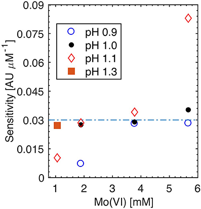
Figure 3. Effect of Mo(VI) concentration and pH on analytical sensitivity. Symbols above the dashed line were characterized with a high reagent blank, highlighting inadequate Mo(VI) and pH reaction conditions (see text for details). The orange square represents the Mo(VI) and pH pair adopted in this study. Analytical sensitivity defined as the slope of a calibration curve (0, 1, 2 μM ${\text{PO}}_4^{3-}$) obtained using Sensor 1 (41 mm measurement cells) at each Mo(VI) and pH condition evaluated.

The maximum, blank free, analytical sensitivity of ~0.03 AU μM⁻¹ can be reached at any of the four Mo(VI) concentrations tested (Figure 3), as long as the reaction pH is low enough to mitigate the reagent blank and Si interference that occur at elevated Mo(VI) concentrations. To minimize the amount of Mo(VI) and sulfuric acid needed to prepare the molybdate reagent, R1 was prepared to obtain a reaction pH of 1.3 and a Mo(VI) concentration of 1.1 mM following diffusional mixing with the sample in the sensor measurement cells. This procedure corresponds to a reaction [Mo(VI)]/[H⁺] ratio of 41, which is identical to that used in Patey et al. (2010) and Zimmer and Cutter (2012) Continuous Segmented Flow Analysis methods. Note, however, that the reaction pH and [Mo(VI)]/[H⁺] ratio reported in Patey et al. (2010) are incorrect, as the authors appear to have assumed that both H₂SO₄ protons fully dissociate in dilute solutions (the second dissociation constant of H₂SO₄ is very small relative to the first one).

Silicate Interferences

After selecting a suitable Mo(VI) concentration and pH pair, the potential for silicate interferences was revisited by comparing the absorbance of UHP water samples spiked with phosphate against that of samples spiked with both ${\text{PO}}_4^{3-}$ and Si(OH)₄. The concentration of Si(OH)₄ (2–300 μM) and ${\text{PO}}_4^{3-}$ (0.1–3 μM) in the test solutions was chosen in order to replicate the range of concentrations likely to occur in surface, thermocline, and deep ocean waters. At the three concentration ranges tested, there were no significant differences in the absorbance of the ${\text{PO}}_4^{3-}$ and ${\text{PO}}_4^{3-}$ + Si(OH)₄ additions (two sample t-test, P > 0.2, df = 4), further confirming that that the selected reaction Mo(VI) concentration and pH maximize sensitivity to phosphate while mitigating silicate interference.

Ascorbic Acid and PVP Dispersant

While the Mo(VI) concentration and acidity of the reaction must be carefully optimized, the molybdenum blue assay tolerates a much greater range of ascorbic acid concentrations (Nagul et al., 2015). To maximize the reaction rate, a 19 mM ascorbic acid concentration was adopted. Increasing the ascorbic acid concentration past 19 mM did not improve the kinetics of the reaction nor its sensitivity over a 300 s stopped flow period (data not shown). Lowering the ascorbic acid concentration to 2.4 mM (Zhang and Chi, 2002; Patey et al., 2010; Zimmer and Cutter, 2012), led to a 15% reduction in analytical sensitivity relative to that obtained with 19 mM ascorbic acid in the reaction mixture (data not shown).

Note that it is critical to prepare the ascorbic reagent with a dispersant in order to mitigate adsorption of the reaction products onto the walls of the chip microfluidic channels. Without dispersant, the analytical sensitivity of the sensor was up to six times lower and did not produce a linear relationship between phosphate concentration and absorbance, presumably because of the aforementioned wall effects. While the sensor can operate adequately at room temperature using Sodium Dodecyl Sulfate (SDS) as a surfactant, precipitation of SDS at temperatures less than ~17°C renders this surfactant unsuitable for in situ operations in most environments (Adornato et al., 2007). For this reason, Clinton-Bailey et al. (2017) recommended adding 0.01% (w/v) polyvynilpyrrolidone (PVP) to the ascorbic reagent since PVP is stable at low temperatures and yields linear calibration results of adequate sensitivity (albeit lower than that obtained with SDS). Interestingly, the need for a dispersant such as PVP or SDS in the reacting mixture appears to be specific to microfluidic instruments, considering that several mesofluidic flow methods operate satisfactorily without surfactant (Wu et al., 2001; Mesquita et al., 2011; Ma et al., 2014). This is likely due to the fact that microfluidic instruments have a surface area to volume ratio two or more orders of magnitude higher than mesofluidic instruments.

Temperature Effects

The analytical performance of Sensor 1 was determined at six different temperatures ranging from 5 to 30°C. During these experiments, the sensor and reagents were placed in a temperature controlled chamber, allowed to equilibrate to the chamber temperature overnight and programmed to run a calibration with a 300 s reaction time the next day (0, 1, 2, and 3 μM ${\text{PO}}_4^{3-}$ in UHP water). Figure 4A shows that analytical sensitivity increases linearly from 5 to 25°C (slope = 6 × 10⁻⁴ AU μM⁻¹ °C⁻¹) prior to reaching a plateau at temperatures >25°C, consistent with the anticipated influence of temperature on the kinetics of the molybdenum blue reaction (Sjösten and Blomqvist, 1997). The Limit of Detection (LOD) of Sensor 1 [defined as three times the blank baseline noise (n = 5)] was 4.0 × 10⁻⁴ AU at 5°C and 6.5 × 10⁻⁴ AU at 25°C. These figures correspond to LODs for phosphate of 40 and 30 nM at 5 and 25°C, respectively, and confirm that the sensor provides a high degree of precision at low temperatures, even if analytical sensitivity decreases. On the other hand, the LOD calculations also show that ambient temperature variations of about one degree Celsius have the potential to produce a small, yet detectable, change in absorbance (i.e., ~6 × 10⁻⁴ AU °C⁻¹ for a 1 μM ${\text{PO}}_4^{3-}$ solution). However, such changes should not impact the infield accuracy of the sensor, considering that each sample analyzed is calibrated against one or two standards in situ.

FIGURE 4

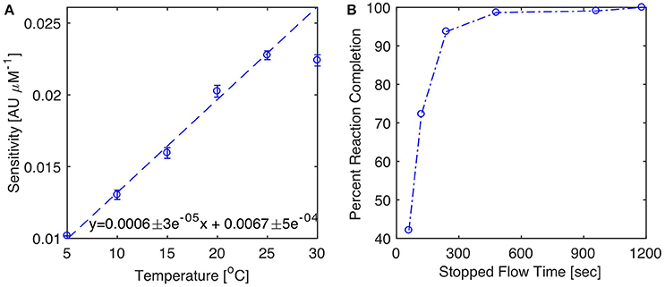
Figure 4. Impact of temperature and reaction time on analytical sensitivity. (A) Analytical sensitivity vs. incubation temperature. Analytical sensitivity defined as slope ± 1 S.E of calibration curves ran at each temperature with a 300 s reaction time. The inset equation is the linear regression between temperature and sensitivity from 5 to 25°C (dashed line). (B) Percent reaction completion at 20°C as a function of length of stopped flow period. The percent reaction completion is defined as the slope of calibration curves obtained at each stopped-flow time (60, 120, 240, 480, 960, 1,180 s) normalized by the slope of the calibration at 1,180 s. This assumes that the reaction is complete after a reaction time of 1,180 s.

Analytical sensitivity increased with the length of time the analyte and reagents are left to react in the measurement cells. At ambient laboratory temperature (20°C), color production is more than 95% complete following a 300 s stopped flow period (Figure 4B). It is not necessary to wait for reaction completion to determine the absorbance and compute sample phosphate concentrations. For example, halving the reaction time will decrease analytical sensitivity by about 30% (Figure 4B), while improving the sensor measurement frequency by 10 min. This approach was successfully implemented during the Nutrient Sensor Challenge, in order to achieve a sampling frequency shorter than 30 min per sample.

Optical Correction: Salinity and Sample Color

Although the analytical sensitivity of the molybdenum blue assay is unaffected by the ionic strength of the sample matrix (Murphy and Riley, 1962; Nagul et al., 2015), a bias will occur if the sensor is operated with onboard blank and standards of different ionic strength than that of the sample analyzed. This effect is illustrated in Figure 5, which displays the measured phosphate concentration of samples of different salinities (0–30) and spiked with the same concentration of phosphate (1.67 μM), while the sensor was operated with blank and standard solutions prepared in UHP water (S = 0). Under these conditions, increasing the salinity of the sample produced an underestimation of the true phosphate concentration, with an error of about −20% at full salinity (S = 35, Figure 5). This salinity bias is purely optical and arises because of matrix dependent variations in light transmission through the measurement cells (Mesquita et al., 2011). At higher sample salinities, the incoming light is better directed toward the photodiode detector compared to deionized water samples. For this reason, photodiode voltages are always higher when the measurement cells are filled with seawater compared to deionized water. As such, at equal phosphate concentrations, the absorbance of a reacted seawater sample will always be lower than that of deionized water, thereby producing a concentration offset when sample concentration is computed.

FIGURE 5

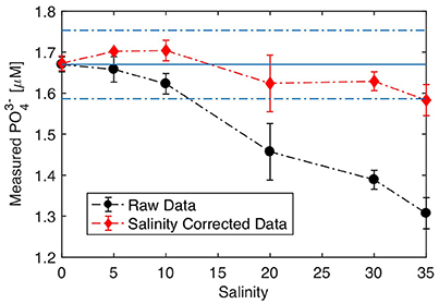
Figure 5. Salinity response. Sensor operating using onboard standard and blanks prepared in UHP water. Samples were prepared by serial dilutions of low nutrient seawater, which was spiked with 1.67 μM ${\text{PO}}_4^{3-}$ at each salinity tested. The solid and dashed lines represent the spiked ${\text{PO}}_4^{3-}$ concentration in the sample ± 5%, respectively. Error bars represent the standard deviation of replicate analyses (n = 3).

This salinity bias can be corrected in situ by recording the photodiode voltages when the measurement cells are filled with blank and sample solution during the manifold flushing steps that precede the injection of the reagents and the color development (Table S1). With this information, an absorbance offset is calculated and then subtracted from the absorbance of the sample recorded after color development. Figure 5 shows that applying this correction scheme allows the sensor to maintain an accuracy of 5% (i.e., ± 0.08 μM) across the full salinity range when it is operated with blanks and standards prepared in UHP water. This optical correction is particularly useful for deployments in estuarine regions or when the operator does not have access to low nutrient seawater to prepare the blanks and standards. Note that a similar optical correction scheme may be applied for the analysis of colored (e.g., high CDOM) samples.

Nevertheless, it is recommended to match the salinity of the onboard blank and standards to the median salinity expected at the deployment location. If the salinity of the onboard solutions is properly adjusted, Figure 5 suggests that the sensor can tolerate salinity fluctuations on the order of ±10 salinity units without correction.

Calibration, LODs, CRM Analysis, and Sensor Endurance

Figure 6 displays typical photodiode reaction rate curves obtained during a 300 s stopped flow period and the calibration graph produced using low nutrient seawater spiked with phosphate (0.12, 0.25, 0.50 μM ${\text{PO}}_4^{3-}$) for the three measurement channels of Sensor 2. These data were obtained in the laboratory prior to the deployment of Sensor 2 in the field. The reaction rate curves show that color formation is rapid, considering that the photodiode voltages of the reacted blank and standard solutions are already significantly different (>10 mV) after ~60 s reaction time (Figure 6A). The gradual decrease in the voltages of the standard solutions from 60 to 300 s confirm that longer reaction times provide higher sensitivity and lower LODs (Figure 6A).

FIGURE 6

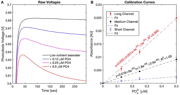
Figure 6. Pre-deployment sensor performance evaluation using acidified low nutrient seawater spiked with 0.12, 0.25, and 0.5 μM ${\text{PO}}_4^{3-}$. (A) Example voltages recorded during a 300 s stopped flow period from the medium channel, (B) pre-deployment calibration curves for the long, medium, and short channels.

After a 300 s stopped flow period, the analytical sensitivity of the long channel was ~2.8 times higher than the medium channel, consistent with Beer-Lambert's law (Figure 6B). The short channel (2.5 mm), which features a LOD around 0.5 μM Clinton-Bailey et al. (2017), is not sensitive enough for the low PO₄ concentrations tested in Figure 6. The LOD of the long and medium channels was 30 nM, similar to that reported by Clinton-Bailey et al. (2017) with a prototype phosphate sensor with 41 mm cells optimized for freshwater deployments. The LOD of the long channel of Sensor 2 was not consistently lower than the medium channel in spite of the higher analytical sensitivity of the long channel, indicating that optical noise may have scaled with the length of the measurement cell.

As part of the optimization work, the accuracy of Sensors 1 and 2 was determined in the laboratory by analyzing Certified Reference Materials (CRM, Kanso Co. Ltd., Japan). Table 1 shows that the accuracy of both sensors was better than 6% for the CD and BW reference samples. The accuracy is defined as the absolute percent error with respect to the CRMs certified values provided by Kanso.

TABLE 1

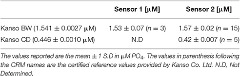
Table 1. Analysis of Kanso Certified Reference Material (CRM) using Sensors 1 and 2.

With the volumes of reagents and standards described in Section Reagent Preparation and when connected to shore power, the sensor can operate in situ for 60-days with an hourly measurement frequency. However, in highly turbid environments, the intake filter may need to be replaced prior to exhaustion of the reagents. Since the reagent consumption (Table S3) is proportional to the sampling rate, the endurance of the sensor may be extended by decreasing the sampling rate. For remote operation, the sensor can be powered using a custom-made 78 Ah, 12 V battery pack. Using such a battery pack, the sensor must be set to sample every 3 h to provide a field endurance of 60 days.

Laboratory Tank Testing

Table 2 summarizes the Sensor and reference method phosphate concentrations obtained at the 17 exposure conditions tested in a 250 L tank as part of the Nutrient Sensor Challenge. A model II regression line was fitted to the paired sensor and reference method phosphate data (n = 62) at all but the highest phosphate concentration (~60 μM) tested, which was beyond the linear quantification range of the sensor (discussed below). The fit indicates that the LOC sensor measurements are accurate to ±0.13 μM (root mean square error of Type II regression) with a measurement accuracy around 5% across the range of exposure conditions tested (Sensor-PO₄ = 0.95 ± 0.005 × Reference-PO₄ + 0.06 ± 0.02 μM, 95% C.I, Figure 7). The sensor precision, calculated using replicate analyses of the tank water at each exposure condition, was lower than 6% at phosphate concentrations >0.3 μM and around 10% below that (Table 2). The excellent agreement between the reference and sensor tank measurements at high salinities, suspended particulate matter (SPM) and CDOM concentrations further confirms that the in situ optical correction protocol allows the sensor to operate in a variety of natural waters while maintaining high precision and accuracy (Table 2). The sensor performance at low temperatures (5°C) was also satisfactory, even though values were biased low relative to the standard method at phosphate concentrations >0.3 μM (Table 2).

TABLE 2

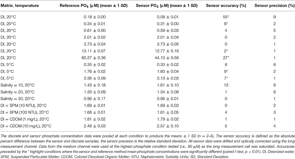
Table 2. Analytical performance of Sensor 2 while immersed in a 250 L tank.

FIGURE 7

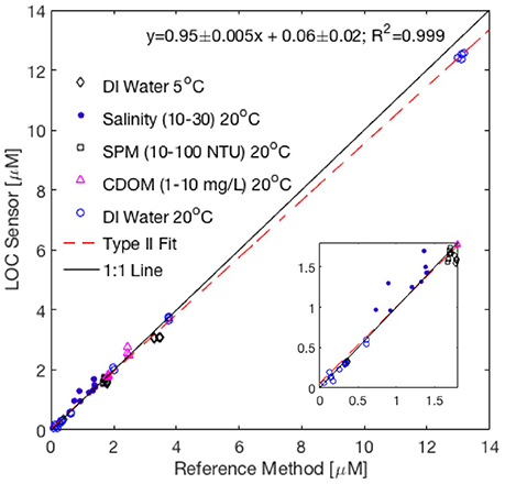
Figure 7. Comparison of phosphate concentrations determined using Sensor 2 and values obtained using USEPA Reference method No 365.5 at the 17 exposure conditions tested as part of the Nutrient Sensor Challenge (n = 62). Also included are reference and sensor measurements performed at the beginning of each day of testing, when the test tank was filled with deionized water (as low as 0.06 μM ${\text{PO}}_4^{3-}$). Data from the highest phosphate concentration tested (60 μM) are not shown nor included in the fit (see text for details). The dashed shows the Type II Linear Regression between sensor and reference method. The inset graph plots the same data at a reduced scale. DI, Deionized water; SPM, Suspended Particulate Matter; NTU, Nephelometric Turbidity Units; CDOM, Colored Dissolved Organic Matter.

The worst agreement between the sensor and reference method occurred at the lowest and highest phosphate concentrations tested (Table 2). At the highest exposure (~60 μM), the long measurement cell was saturated (absorbance >1.7) while the medium and short channels showed no sign of optical saturation (absorbance <0.2). For this reason, the underestimated phosphate concentrations reported by the sensor are most likely due to a limiting concentration of one of the reagents in the reacting mixture. Nagul et al. (2015) showed that the upper end of the linear calibration range of the molybdenum blue reaction occurs when the Sb(III):P ratio becomes <2. With 60 μM phosphate in the tank water, the Sb(III):P ratio in the sensor measurement cells following complete diffusional mixing was 1.87, suggesting that Sb(III) was limiting. As such, in order to operate the sensor near 60 μM phosphate, R1 would need to be prepared with a slightly higher concentration of PAT. Note, however, that such concentrations of phosphate are unlikely to be encountered in any but severely polluted waters.

It is unclear what caused the poor accuracy of the sensor at the lowest phosphate concentration listed in Table 2, considering that the reference and sensor data showed good agreement at the beginning of one of the test days, when the 250 L tank was filled with deionized water (reference = 0.06 μM, sensor: 0.05 μM, data included in Figure 7). Since the sensor operated using only one standard (0.5 or 15 μM) during the tank tests to maintain a 30 min sampling interval, an intermittent calibration issue cannot be entirely ruled out. For this reason, when the sensor is deployed in oligotrophic systems, it is best to operate the sensor using two standards that bracket the expected concentration range at the deployment site.

Field Deployments

Empress Dock, Southampton Water

Southampton Water is a macrotidal, partially mixed estuary located on the south coast of the UK (Figure S1). It receives freshwater inputs from the Rivers Test and Itchen and discharges into the English Channel via the Solent, north of the Isle of Wight. The estuary has been referred to as a hypernutrified system, with elevated nutrient levels maintained by inputs from the Rivers Itchen and Test combined with consented wastewater discharges along its upper reaches (Hydes and Wright, 1999; Holley et al., 2007). Relative to the Test, the River Itchen is more impacted by land use and point source inputs, with phosphate concentrations on the order of 7 μM reported at the saltwater intrusion limit in spring 1998 (Xiong, 2000).

Figure 8 shows phosphate data from the first deployment of Sensor 1 in Southampton Water, during which the sensor performed 1,267 unattended in situ measurements at hourly intervals over a 56-day period. The phosphate concentrations ranged from 0.09 to 2.80 μM (mean ± 1 SD = 1.02 ± 0.40 μM), reached a peak near April 2 coinciding with a 2-fold drop in salinity and showed a pronounced decrease during the last week of April overlapping with an increase in dissolved oxygen (Figure 8). The discrete and sensor data showed broadly coherent trends throughout the deployment period (Figure 8); the infield accuracy of the sensor was superior during the first month of deployment (5 ± 3%, mean ± 1 SD) compared to the second month. The Type II regression between the sensor and reference data (y = 0.90 ± 0.04x + 0.15 ± 0.05; R² = 0.925) suggests that the sensor data in Southampton Water were accurate to ± 0.10 μM relative to the reference data, similar to the value obtained during the laboratory tank tests (0.12 μM). A paired t-test showed that the sensor and reference data were significantly different (p < 0.01, df = 60), with the sensor data displaying a positive bias that was more pronounced after April 20 (Figure 8). However, if only the values prior to April 20 are considered (i.e., the first 36 days of deployment), the sensor and reference data were no longer significantly different (paired t-test, p = 0.08, df = 44). It is unclear what caused the higher bias in some of the sensor values past April 20 (Figure 8), since the ancillary sensor data (i.e., voltages of blank and standard) did not exhibit significant drift past that date. Nevertheless, as discussed below, the general trends recorded by the phosphate sensor past April 20 were still consistent with the salinity, oxygen, and tidal data (Figure 8).

FIGURE 8

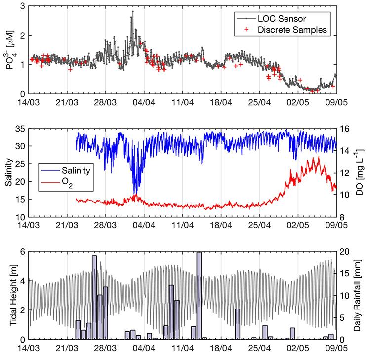
Figure 8. Fifty-six-day time series of phosphate and environmental parameters at Empress Dock, Southampton Water in Spring 2016. (Top) Hourly phosphate sensor data (n = 1,267) and discrete samples (n = 61). (Middle) YSI Salinity and oxygen (5 min sampling frequency). (Bottom) Tide data from SOTONMET (Associated British Ports) and daily rainfall in Southampton City (bars). Rain data from http://www.southamptonweather.co.uk.

Enhanced discharge of nutrient-rich river water and associated urban runoff during storm events can have a significant impact on nutrient concentrations in Southampton Water (Hydes and Wright, 1999; Beaton et al., 2012). Such a storm event occurred from March 26 to 28, when daily rainfall >10 mm was recorded for three consecutive days (Figure 8). This rain event was accompanied by a drop in salinity and increased phosphate concentrations (up to 1.95 μM on March 29) lasting about 4 days at the Empress Dock (Figure 8). Interestingly, the highest phosphate concentrations (2.8 μM on April 2) and lowest salinity (17) of the 8-week time-series occurred during a rain event of significantly lower magnitude (Apr 1–3; Figure 8). However, the latter event occurred during the neap tide (Figure 8), when the fraction of nutrient-rich river water in Southampton Water was significantly greater than that of low nutrient English Channel water. The spring-neap tidal cycle can also be invoked to explain the absence of a pronounced phosphate and salinity signal following the rain event centered on April 9 (Figure 8), which occurred in the middle of the spring tide and was probably buffered by enhanced mixing with low nutrient seawater. Thus, while storm events clearly have an impact on water quality in Southampton Water, the magnitude of these impacts appears to be modulated by the spring-neap tidal cycle.

On a daily timescale, the phosphate sensor provides adequate precision to resolve tidally driven fluctuations in phosphate concentrations at a fixed location in Southampton Water. Figure 9 expands the phosphate, salinity, and oxygen data from April 22–27, 2016 to highlight the tidal periodicity. During this period, phosphate showed a sinusoidal signal with a period of 12 h and amplitude of about 0.2 μM. Peak phosphate values consistently occurred during or shortly after low water (Figure 9), reflecting the greater fraction of nutrient-rich river water invading the deployment location at low tide.

FIGURE 9

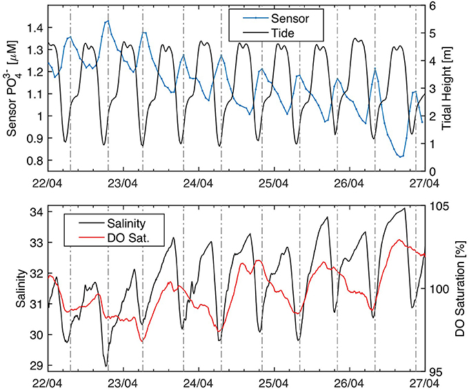
Figure 9. Phosphate tidal cycling at the Empress Dock, Southampton Water. (A) Phosphate and tidal height. (B) YSI salinity and dissolved oxygen. The dashed vertical lines highlight the position of the phosphate maxima recorded by the sensor. A moving average was applied to the sensor (window size = 4) and YSI data (window size = 24). Tide data from SOTONMET (Associated British Ports).

Phosphate and nitrate are generally well correlated with salinity in Southampton Water, except in its upper reaches due to point source discharges and during periods of enhanced biological uptake in spring and summer (Hydes and Wright, 1999; Xiong, 2000). Salinity and phosphate showed an inverse linear correlation during the first 6 weeks of the deployment period (Figure 10), consistent with the notion of conservative mixing in Southampton Water. The salinity-phosphate relationship predicts a river water end member concentration of 3.33 ± 0.06 μM and a Solent Water (S = 34–35) concentration of ~0.9 μM, within the expected range of phosphate concentrations in the Solent prior to the main spring bloom (Holley et al., 2007). Unlike the high-resolution nitrate observations of Beaton et al. (2012) in Southampton Water, the salinity-phosphate relationship prior to and after rain events did not show evidence for dilution of the river end member phosphate concentration during storm events. This suggests that non-point sources of phosphate may have been the dominant source of phosphate to the River Test and Itchen during the deployment period.

FIGURE 10

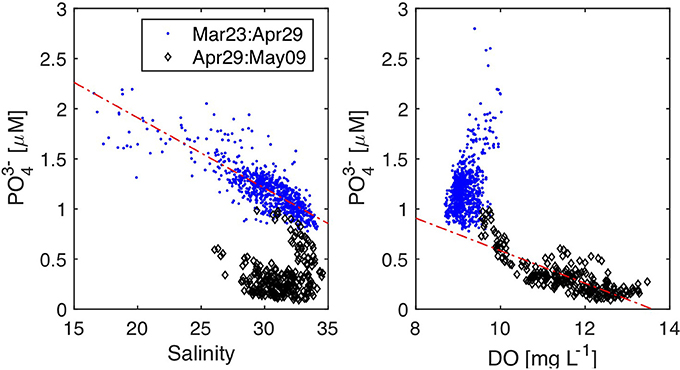
Figure 10. Property-property plots for Southampton Water deployment. (A) Phosphate vs. YSI Salinity y = −0.07 ± 0.002 * x + 3.3 ± 0.06 R² = 0.63 (Mar 23–Apr 29, n = 856), (B) Phosphate vs. YSI Dissolved Oxygen y = −0.16 * x + 2.2 R² = 0.65 (Apr 29–May 09).

Although we did not collect any chlorophyll-a data to estimate biological activity during the deployment, the phosphate and oxygen data strongly suggest that the last 10 days of the Southampton Water deployment were impacted by a spring phytoplankton bloom. After April 29, phosphate concentrations dropped by a factor of 10 over a period of 6 days (Figure 8), reaching values around 0.1 μM on May 4. During the same period, salinity and phosphate were no longer significantly correlated (P > 0.05) while phosphate and dissolved oxygen showed a significant negative correlation (Figure 10). These geochemical considerations strongly suggest that the 10-fold drop in phosphate concentrations recorded by the LOC sensor during the last week of April 2016 was the result of biological uptake. The timing of the 2016 spring bloom in Southampton Water, as evidenced by the phosphate and oxygen data, is consistent with the findings of Iriarte and Purdie (2004), who investigated the timing and magnitude of spring bloom events in the Solent using a 5-year time series.

Kaneohe Bay, Oahu, Hawaii

Figure 11 shows phosphate data from a 31-day deployment in the southern sector of Kaneohe Bay, a semi-enclosed tropical embayment on the windward side of the island of Oahu, Hawaii (Figure S2). Kaneohe Bay is the largest sheltered body of water in the Hawaiian Islands and is relatively oligotrophic, with phosphate concentrations generally <0.2 μM during low rainfall periods (De Carlo et al., 2007; Drupp et al., 2011). Enhanced river discharge associated with storm events can deliver pulses of nutrient-enriched freshwater into the bay, relieving N-limitation and driving short-lived phytoplankton blooms, particularly during light wind conditions that maintain a stratified water column (Drupp et al., 2011 and references therein). However, no significant rainfall event (>0.5 cm) and enhanced river discharge were experienced throughout the deployment period (October 3–November 3, 2016), implying that the biogeochemical condition of Kaneohe Bay was representative of baseline low rainfall season conditions. As such, the phosphate and salinity data were not correlated, even near October 10 when a low salinity plume impacted the deployment site (Figure 11).

FIGURE 11

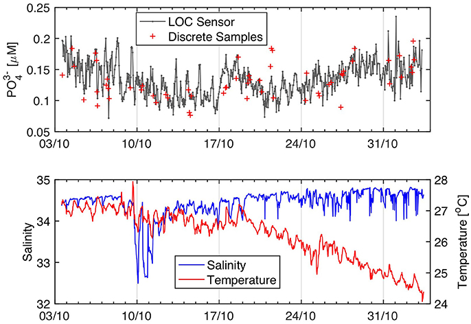
Figure 11. Kaneohe Bay phosphate time-series from Sensor 2. High frequency noise in the salinity data past 20/10 was removed to produce the salinity plot. The phosphate data displayed are from the long channel. The long channel raw voltages were drift corrected to compensate for variations in the intensity of the LEDs. The phosphate concentrations were calculated using a linear regression forced through the origin using the two onboard phosphate standards.

During the 31-day deployment in Kaneohe Bay, Sensor 2 performed 741 hourly phosphate measurements. Five percent of these data (n = 37) were flagged as outliers due to bad standard or blank measurements and are not plotted in Figure 11. The phosphate concentrations recorded by Sensor 2 ranged from 0.07–0.23 μM (0.13 ± 0.03 μM, mean ± 1 SD, n = 704), consistent with the minimal rainfall and river water inputs into the bay during the deployment period. Although the discrete and sensor data were weakly correlated (R² = 0.35), there were no significant differences in the analytical results at the 1% significance level (paired t-test, P = 0.013, df = 56). The standard deviation of the difference between paired sensor and discrete measurements was 0.025 μM, within the error of both methods. Thus, the Kaneohe Bay deployment confirms that Sensor 2 is capable of providing unattended, hourly in situ data of reasonable accuracy (16 ± 12%) relative to reference methods at phosphate levels ranging between 0.1 and 0.2 μM.

While the Kaneohe Bay phosphate time series displays high frequency noise, a closer inspection of the data reveals noteworthy periodical trends, particularly during the second week of deployment (Figure 11). Figure 12 displays data from October 12–16, which were smoothed with a 6 h moving average to remove some of the variability. It shows that, during this time period, phosphate levels tended to peak in the early morning hours (4–8 a.m.) followed by a rapid decline. These observations, although not consistently observed throughout the deployment period, may be interpreted as a diurnal signal driven by biological phosphate uptake during peak daylight hours. However, a tidal influence cannot be entirely ruled out considering that the phosphate peaks with the largest amplitude coincided with the low tide, while high tide conditions were generally associated with lower phosphate concentrations (Figure 12). Thus, it is also possible that the sensor picked up the movement of a nutrient enriched plume of water advecting in and out of the deployment location with the tide. Notwithstanding the origin of this signal, which would require a longer time-series to be confirmed, the Kaneohe Bay time-series further exemplify the utility of sustained high-frequency real time observations to disentangle the impact of overlapping signals on nutrient dynamics.

FIGURE 12

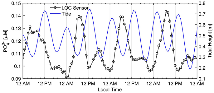
Figure 12. Potential diurnal phosphate variations in Kaneohe Bay. Data from October 12–16, 2016. Sensor phosphate data were smoothed with a 6 h moving average. Tide data from Moku O Loe (Coconut Island) gauging station.

Conclusions and Perspectives

Long-term, high-frequency, in situ observations are crucial to improve our understanding of the fluxes, temporal dynamics and biogeochemical implications of nutrient distributions in coastal and oceanic waters. This work highlights that microfluidic Lab-On-Chip analyzers are mature enough to monitor phosphate at sub-hourly intervals over month long periods with accuracy and precision close to that obtained using state of the art reference methods on discrete samples. Deployments in the hypernutrified Southampton Water estuary and in the oligotrophic tropical waters of Kaneohe Bay highlighted that the sensor can capture stochastic events such as storms, as well as recurring low amplitude phosphate dynamics operating across different time scales. These dynamics, namely the tidal modulation of phosphate concentrations in Southampton Water and a potential phosphate diurnal signal in Kaneohe Bay, further demonstrate that microfluidic wet chemical sensors can provide powerful insights into the biogeochemical variability of natural waters that cannot be captured via traditional discrete sampling.

The optimized phosphomolybdenum blue chemistry and microfluidic sensor architecture described here are well-suited to monitor phosphate in situ in a variety of natural waters. The LOC phosphate sensor features a LOD of 30 nM, linear quantification with a precision better than 10% from 0.05 to 13 μM and a field endurance of ~60 days when the sensor is operated with hourly sampling rate and connected to shore power. The laboratory testing (0.1–12 μM) and field deployment in Southampton Water (0.96 ± 0.4 μM, mean ± 1 SD) showed that the infield accuracy of the sensor was on the order of ± 0.10 μM relative to reference methods. At the oligotrophic site in Kaneohe Bay (0.13 ± 0.03 μM, mean ± 1 SD), the sensor and discrete sample measurements were not statistically different. In addition, the LOC phosphate sensor operated with acceptable precision (<6%) and accuracy (<9%) at temperatures ranging from 5 to 30°C and its analytical performance was unaffected by the salinity, turbidity and CDOM. Thus, LOC phosphate sensors can be deployed in environments ranging from rivers and lakes, to estuaries and coastal waters without user intervention for at least a month.

The production of miniaturized, robust, and easy to use sensors featuring an analytical performance comparable to reference methods are the principal factors that will encourage widespread utilization of in situ sensors by academics and resource managers.

In its present configuration, the figures of merit of the LOC phosphate sensor, its low power consumption (1.8 W) and endurance in the field (30–60 days) make it a viable candidate to instrument cabled observatories and ocean time series sites that are occupied on a monthly basis. The deployment of LOC sensors at ocean time series sites would allow capturing short term variability in nutrient concentrations between monthly discrete sampling events, thus greatly improving temporal resolution without impeding the high quality datasets that have been and will continue to be obtained via monthly discrete shipboard sampling (Karl, 2014). With further testing at low temperatures (<5°C) and using an oil filled pressure compensated housing, the LOC sensor could also be deployed in the deep ocean and appended to deep ocean observatories.

Author Contributions

MG compiled, processed, and interpreted all the field and laboratory sensor data, designed the chemical optimization experiments, and wrote the paper, with edits and contributions from all co-authors. GC identified the potential of PVP for in situ phosphate determinations and collaborated with MG during the chemical optimization. AB and AS designed and developed the sensors. TJ and MT designed and helped conduct the Nutrient Sensor Challenge laboratory and field testing. EA, DC, and MM directed the study and its scope.

Funding

The research leading to these results has received funding from the European Union Seventh Framework Programme (FP7/2007-2013) under grant agreement n°614141 (SenseOCEAN).

Conflict of Interest Statement

The authors declare that the research was conducted in the absence of any commercial or financial relationships that could be construed as a potential conflict of interest.

Acknowledgments

We thank Urska Martincic, Greg Slavik, and Dave Owsianka (NOCS) who collectively manufactured the two sensors used in this study. Thanks are due to John Walk (NOCS) for his support with the sensor GUI and his willingness to fix unavoidable bugs at odd hours and in record time. The laboratory and field help of David Loewensteiner (CBL), Daniel Schar (HIMB), and Heidi Purcell (ACT) during the Nutrient Sensor Challenge is greatly appreciated. MG would like to thank Chris Measures and Mariko Hatta for providing office and lab space at the University of Hawaii at Mānoa, where this paper was written. We thank the two reviewers for their constructive feedback. This manuscript is contribution number 1116 from the Cooperative Institute for Great Lakes Research, University of Michigan.

Supplementary Material

The Supplementary Material for this article can be found online at: https://www.frontiersin.org/article/10.3389/fmars.2017.00255/full#supplementary-material

Figure S1. Southampton water map. The sensor deployment location is shown with the red arrow. Imagery from Google Earth.

Figure S2. Map of Kaneohe Bay, Oahu, Hawaii. The deployment location, on the southwestern side of Coconut Island (Moku O Loe) is highlighted with the red circle. Imagery from Google Earth.

Table S1. Sensor analytical protocol when operated with two onboard standards.

Table S2. Target tank exposure conditions of the Nutrient Sensor Challenge laboratory tests.

Table S3. Reagents, blank, and standard(s) solutions consumption per analytical run (see Table S1). Also listed is the sample waste production, which includes the volume of sample used for flushing the microfluidic channels and analysis and is stored in the flexible waste bag.

References

ACT (2017). Performance Verification Statement for the NOC Phosphate Analyzer. ACT Code CBL 2017-049. Solomons, MD: Alliance for Coastal Technologies. Available online at: http://www.act-us.info/evaluations.php

Adornato, L. R., Kaltenbacher, E. A., Greenhow, D. R., and Byrne, R. H. (2007). High-resolution in situ analysis of nitrate and phosphate in the oligotrophic ocean. Environ. Sci. Technol. 41, 4045–4052. doi: 10.1021/es0700855

PubMed Abstract | CrossRef Full Text | Google Scholar

Barus, C., Romanytsia, I., Striebig, N., and Garçon, V. (2016). Toward an in situ phosphate sensor in seawater using Square Wave Voltammetry. Talanta 160, 417–424. doi: 10.1016/j.talanta.2016.07.057

PubMed Abstract | CrossRef Full Text | Google Scholar

Beaton, A. D., Cardwell, C. L., Thomas, R. S., Sieben, V. J., Legiret, F.-E., Waugh, E. M., et al. (2012). Lab-on-chip measurement of nitrate and nitrite for in situ analysis of natural waters. Environ. Sci. Technol. 46, 9548–9556. doi: 10.1021/es300419u

PubMed Abstract | CrossRef Full Text | Google Scholar

Benitez-Nelson, C. R. (2000). The biogeochemical cycling of phosphorus in marine systems. Earth Sci. Rev. 51, 109–135. doi: 10.1016/S0012-8252(00)00018-0

CrossRef Full Text | Google Scholar

Bricker, S. B., Longstaff, B., Dennison, W., Jones, A., Boicourt, K., Wicks, C., et al. (2008). Effects of nutrient enrichment in the nation's estuaries: a decade of change. Harmful Algae 8, 21–32. doi: 10.1016/j.hal.2008.08.028

CrossRef Full Text | Google Scholar

Clinton-Bailey, G. S., Grand, M. M., Beaton, A. D., Nightingale, A. M., Owsianka, D. R., Slavik, G. J., et al. (2017). A lab-on-chip analyzer for in situ measurement of soluble reactive phosphate: improved phosphate blue assay and application to fluvial monitoring. Environ. Sci. Technol. doi: 10.1021/acs.est.7b01581. [Epub ahead of print].

PubMed Abstract | CrossRef Full Text | Google Scholar

De Carlo, E. H., Hoover, D. J., Young, C. W., Hoover, R. S., and Mackenzie, F. T. (2007). Impact of storm runoff from tropical watersheds on coastal water quality and productivity. Appl. Geochem. 22, 1777–1797. doi: 10.1016/j.apgeochem.2007.03.034

CrossRef Full Text | Google Scholar

Drupp, P., De Carlo, E. H., Mackenzie, F. T., Bienfang, P., and Sabine, C. L. (2011). Nutrient inputs, phytoplankton response, and CO₂ variations in a semi-enclosed subtropical embayment, Kaneohe Bay, Hawaii. Aquat. Geochem. 17, 473–498. doi: 10.1007/s10498-010-9115-y

CrossRef Full Text | Google Scholar

Floquet, C. F., Sieben, V. J., Milani, A., Joly, E. P., Ogilvie, I. R. G., Morgan, H., et al. (2011). Nanomolar detection with high sensitivity microfluidic absorption cells manufactured in tinted PMMA for chemical analysis. Talanta 84, 235–239. doi: 10.1016/j.talanta.2010.12.026

PubMed Abstract | CrossRef Full Text | Google Scholar

Holley, S., Purdie, D., Hydes, D., and Hartman, M. (2007). 5 Years of Plankton Monitoring in Southampton Water and the Solent Including FerryBox, Dock Monitor and Discrete Sample Data. UK National Oceanography Centre Southampton.

Google Scholar

Hydes, D. J., and Wright, P. (1999). SONUS: The Southern Nutrients Study 1995-1997. Southampton: UK Southampton Oceanography Centre.

Google Scholar

Iriarte, A., and Purdie, D. A. (2004). Factors controlling the timing of major spring bloom events in an UK south coast estuary. Estuar. Coast. Shelf Sci. 61, 679–690. doi: 10.1016/j.ecss.2004.08.002

CrossRef Full Text | Google Scholar

Johnson, K. S., Riser, S. C., and Karl, D. M. (2010). Nitrate supply from deep to near-surface waters of the North Pacific subtropical gyre. Nature 465, 1062–1065. doi: 10.1038/nature09170

PubMed Abstract | CrossRef Full Text | Google Scholar

Jońca, J., Comtat, M., and Garçon, V. (2013a). In Situ Phosphate Monitoring in Seawater: Today and Tomorrow. Berlin; Heidelberg: Springer.

Google Scholar

Jońca, J., Giraud, W., Barus, C., Comtat, M., Striebig, N., Thouron, D., et al. (2013b). Reagentless and silicate interference free electrochemical phosphate determination in seawater. Electrochim. Acta 88, 165–169. doi: 10.1016/j.electacta.2012.10.012

CrossRef Full Text | Google Scholar

Jońca, J., León Fernández, V., Thouron, D., Paulmier, A., Graco, M., and Garçon, V. (2011). Phosphate determination in seawater: toward an autonomous electrochemical method. Talanta 87, 161–167. doi: 10.1016/j.talanta.2011.09.056

PubMed Abstract | CrossRef Full Text | Google Scholar

Karl, D. M. (2014). Microbially mediated transformations of phosphorus in the sea: new views of an old cycle. Ann. Rev. Mar. Sci. 6, 279–337. doi: 10.1146/annurev-marine-010213-135046

PubMed Abstract | CrossRef Full Text | Google Scholar

Legiret, F. E., Sieben, V. J., Woodward, E. M., Abi Kaed Bey, S. K., Mowlem, M. C., Connelly, D. P., et al. (2013). A high performance microfluidic analyser for phosphate measurements in marine waters using the vanadomolybdate method. Talanta 116, 382–387. doi: 10.1016/j.talanta.2013.05.004

PubMed Abstract | CrossRef Full Text | Google Scholar

Ma, J., Li, Q., and Yuan, D. (2014). Loop flow analysis of dissolved reactive phosphorus in aqueous samples. Talanta 123, 218–223. doi: 10.1016/j.talanta.2014.02.020

PubMed Abstract | CrossRef Full Text | Google Scholar

Mesquita, R. B., Ferreira, M. T., Tóth, I. V., Bordalo, A. A., McKelvie, I. D., and Rangel, A. O. (2011). Development of a flow method for the determination of phosphate in estuarine and freshwaters–comparison of flow cells in spectrophotometric sequential injection analysis. Anal. Chim. Acta 701, 15–22. doi: 10.1016/j.aca.2011.06.002

PubMed Abstract | CrossRef Full Text | Google Scholar

Murphy, J., and Riley, J. P. (1962). A modified single solution method for the determination of phosphate in natural-waters. Anal. Chim. Acta 27, 31–36. doi: 10.1016/S0003-2670(00)88444-5

CrossRef Full Text | Google Scholar

Nagul, E. A., McKelvie, I. D., Worsfold, P., and Kolev, S. D. (2015). The molybdenum blue reaction for the determination of orthophosphate revisited: opening the black box. Anal. Chim. Acta 890, 60–82. doi: 10.1016/j.aca.2015.07.030

PubMed Abstract | CrossRef Full Text | Google Scholar

National Research Council (2000). Clean Coastal Waters: Understanding and Reducing the Effects of Nutrient Pollution. Washington, DC: National Academies Press.

Nightingale, A. M., Beaton, A. D., and Mowlem, M. C. (2015). Trends in microfluidic systems for in situ chemical analysis of natural waters. Sens. Actuat. B Chem. 221, 1398–1405. doi: 10.1016/j.snb.2015.07.091

CrossRef Full Text | Google Scholar

Ogilvie, I. R. G., Sieben, V. J., Floquet, C. F. A., Zmijan, R., Mowlem, M. C., and Morgan, H. (2010). Reduction of surface roughness for optical quality microfluidic devices in PMMA and COC. J. Micromech. Microeng. 20:65016. doi: 10.1088/0960-1317/20/6/065016

CrossRef Full Text | Google Scholar

Patey, M. D., Achterberg, E. P., Rijkenberg, M. J., Statham, P. J., and Mowlem, M. (2010). Interferences in the analysis of nanomolar concentrations of nitrate and phosphate in oceanic waters. Anal. Chim. Acta 673, 109–116. doi: 10.1016/j.aca.2010.05.029

PubMed Abstract | CrossRef Full Text | Google Scholar

Paytan, A., and McLaughlin, K. (2007). The oceanic phosphorus cycle. Chem. Rev. 107, 563–576. doi: 10.1021/cr0503613

PubMed Abstract | CrossRef Full Text | Google Scholar

Pellerin, B. A., Bergamaschi, B. A., Gilliom, R. J., Crawford, C. G., Saraceno, J., Frederick, C. P., et al. (2014). Mississippi river nitrate loads from high frequency sensor measurements and regression-based load estimation. Environ. Sci. Technol. 48, 12612–12619. doi: 10.1021/es504029c

PubMed Abstract | CrossRef Full Text | Google Scholar

Pellerin, B. A., Stauffer, B. A., Young, D. A., Sullivan, D. J., Bricker, S. B., Walbridge, M. R., et al. (2016). Emerging tools for continuous nutrient monitoring networks: sensors advancing science and water resources protection. J. Am. Water Resour. Assoc. 52, 993–1008. doi: 10.1111/1752-1688.12386

CrossRef Full Text | Google Scholar

Sieben, V. J., Floquet, C. F. A., Ogilvie, I. R. G., Mowlem, M. C., Morgan, H., Izuo, S., et al. (2010). Microfluidic colourimetric chemical analysis system: application to nitrite detection. Anal. Methods 2, 484. doi: 10.1039/c002672g

CrossRef Full Text | Google Scholar

Sjösten, A., and Blomqvist, S. (1997). Influence of phosphate concentration and reaction temperature when using the molybdenum blue method for determination of phosphate in water. Water Res. 31, 1818–1823. doi: 10.1016/S0043-1354(96)00367-3

CrossRef Full Text | Google Scholar

Thouron, D., Vuillemin, R., Philippon, X., Lourenço, A., Provost, C., Cruzado, A., et al. (2003). An autonomous nutrient analyzer for oceanic long-term in situ biogeochemical monitoring. Anal. Chem. 75, 2601–2609. doi: 10.1021/ac020696+

PubMed Abstract | CrossRef Full Text | Google Scholar

Wild-Allen, K., and Rayner, M. (2014). Continuous nutrient observations capture fine-scale estuarine variability simulated by a 3D biogeochemical model. Mar. Chem. 167, 135–149. doi: 10.1016/j.marchem.2014.06.011

CrossRef Full Text | Google Scholar

Wu, C., Ruzicka, J., Blue, I., Epa, T., Yellow, M., Blue, M., et al. (2001). Micro sequential injection: environmental monitoring of nitrogen and phosphate in water using a “Lab-on-Valve” system furnished with a microcolumn. Analyst 126, 1947–1952. doi: 10.1039/b104305f

PubMed Abstract | CrossRef Full Text | Google Scholar

Xiong, J. (2000). Phosphorus Biogeochemistry and Models in Estuaries: Case Study of the Southampton Water System. Ph.D. Thesis, University of Southampton, School of Ocean and Earth Science, 228. Available online at: https://eprints.soton.ac.uk/42178/

Yücel, M., Beaton, A. D., Dengler, M., Mowlem, M. C., Sohl, F., and Sommer, S. (2015). Nitrate and nitrite variability at the seafloor of an oxygen minimum zone revealed by a novel microfluidic in-situ chemical sensor. PLoS ONE 10:e0132785. doi: 10.1371/journal.pone.0132785

PubMed Abstract | CrossRef Full Text | Google Scholar

Zhang, J.-Z., and Chi, J. (2002). Automated analysis of nanomolar concentrations of phosphate in natural waters with liquid waveguide. Environ. Sci. Technol. 36, 1048–1053. doi: 10.1021/es011094v

PubMed Abstract | CrossRef Full Text | Google Scholar

Zimmer, L. A., and Cutter, G. A. (2012). High resolution determination of nanomolar concentrations of dissolved reactive phosphate in ocean surface waters using long path liquid waveguide capillary cells (LWCC) and spectrometric detection. Limnol. Oceanogr. Methods 10, 568–580. doi: 10.4319/lom.2012.10.568

CrossRef Full Text | Google Scholar