Bergy Bit and Melt Water Trajectories in Godthåbsfjord (SW Greenland) Observed by the Expendable Ice Tracker

1. Introduction

Solid ice calved from tidewater glaciers in Greenland makes up a significant component of the total freshwater flux from the ice sheet to the ocean. The freshwater phase and magnitude of the flux vary, both from one fjord to another and also seasonally within individual fjords. Accurate representation of the spatial and temporal variability of solid and liquid freshwater flux from Greenlandic fjords can be an important parameter in numerical ocean models, as well as models of present and future climate (Martin and Adcroft, 2010) and paleoclimate (Death et al., 2006). Tidewater glaciers in Greenland exhibit considerable variability in overall dimensions, grounding line depth, and calving style (Sulak et al., 2017) and these factors determine the initial sizes of the solid ice that enters the fjord. After calving, fjord-specific characteristics, including, but not limited to, size and extent of ice mélange and hydrodynamics, influence both transport and melting of the ice as it transits the fjord. Thus, the cumulative effects of calving style of the glacier, spatial and temporal variability of surface hydrography, and overall residence time in the fjord, as well as residence times in the mélange and in open water, will determine whether ice melts in the fjord or exits onto the continental shelf.

Recent studies have focused on large (>100 m) icebergs in Greenland waters as icebergs of this scale are easier to detect using remote sensing (Buus-Hinkler et al., 2014; Enderlin and Hamilton, 2014; Enderlin et al., 2016; Sulak et al., 2017) and in situ (Andres et al., 2015) techniques. While such data provide important information about volumes, distributions and the geographical extent of icebergs, they do not provide information about transport. Measurements of iceberg trajectories in Greenlandic fjords are somewhat limited (Amundson et al., 2010; Sutherland et al., 2014; Andres et al., 2015; FitzMaurice et al., 2016). GPS-based observations in fjords (Sutherland et al., 2014; Sulak et al., 2017) and in Baffin Bay (Wagner et al., 2014; Larsen et al., 2015) are biased toward larger and, presumably, more stable icebergs. Larger icebergs have been tagged with GPS trackers both for scientific reasons, as large icebergs have been found to account for most of the solid ice volume in specific fjords (Sulak et al., 2017), as well as logistical reasons. Commercial GPS trackers are typically deployed by helicopter (Sutherland et al., 2014; Larsen et al., 2015; Sulak et al., 2017), which requires a large, stable platform. Furthermore, commercial GPS trackers are relatively expensive and the additional cost of helicopter deployments typically limits the number of units available for deployment.

Bergy bits typically calve from a larger parent iceberg (Savage et al., 2000, 2001). Previous studies of bergy bits were motivated by the threat of collision with ships and offshore installations (Crocker and Cammaert, 1994; Crocker and English, 1998; Savage et al., 2000, 2001; Crocker et al., 2004; Gagnon, 2008; Ralph et al., 2008; Eik and Gudmestad, 2010). Some tidewater glaciers produce ice in the bergy bit size range (Dowdeswell and Forsberg, 1992). Bergy bits, by merit of their smaller size, have shorter life expectancies and usually melt in the fjord (Dowdeswell and Forsberg, 1992). GPS trackers have not yet been used to study bergy bit trajectories in Greenlandic fjords.

In an attempt to advance our general understanding of fjord circulation and ice-ocean interactions, and transport of bergy bits (i.e., L < 40 m) in a sub-Arctic fjord in southwest Greenland in particular, we developed the expendable ice tracker (EXITE). EXITE is an open-source and low-cost GPS tracker constructed from off-the-shelf (OTS) components. EXITE transmits GPS positions at relatively high frequency via satellite. The simple, yet rugged design is intended to decrease the cost barrier previously encountered when deploying more expensive commercial trackers. EXITE was designed for deployment from the smaller work and fishing boats available in Greenlandic fjords to make deployments more affordable.

Here we describe the design and construction of the EXITE beacon and present findings from a recent deployment of 7 beacons near a marine-terminating glacier in Godthåbsfjord (southwest Greenland; Figure 1) in August 2016. In addition to being affordable and simple to construct, EXITE was designed to be buoyant, with the hope of detecting the transition from a bergy bit tracker to a surface drifter through a change in drift characteristics. Preliminary attempts to estimate the transition from an ice tracker to a surface drifter are presented, though the transition can be difficult to detect. The initial deployment demonstrated that the EXITE design can survive as a drifter in areas with high ice concentrations. Therefore, future studies will feature simultaneous deployments of EXITE beacons on bergy bits and in nearby surface waters. The bergy bit and surface water trajectories reveal new and complex variability observed over short temporal and small spatial scales. These data demonstrate the effectiveness of the EXITE beacon and represent the first high-resolution observations of bergy bit trajectories.

FIGURE 1

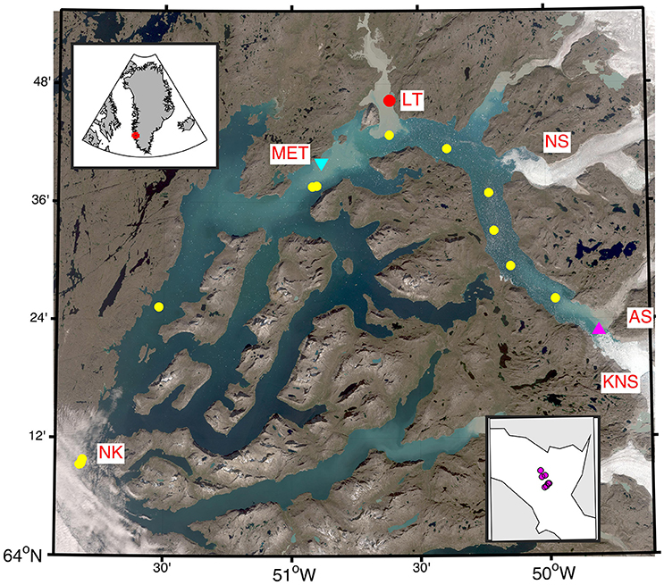
Figure 1. The greater Godthåbsfjord region with the EXITE deployment area near the terminus of the fjord indicated by the pink triangle. The inset at the bottom right shows individual EXITE deployment locations. The inset at the upper left shows the location of Godthåbsfjord (outlined in red) in Greenland. Greenland's capital city of Nuuk (NK) is located near the mouth of the fjord (lower left). CTD profile locations are indicated by yellow circles, with the first profile coinciding with the EXITE deployment location. The location of the Asiaq Greenland Survey meteorological station (MET) is shown by the light blue triangle. The outflow from Lake Tasersuaq (LT) is indicated by a red circle and the turbid outflow plume is visible. The three tidal-outlet glaciers, Narssap Serbia (NS), Akugdlerssûp Serbia (AS), and Kangiata Nunâta Sermia (KNS), are also labeled.

2. Methods

2.1. EXITE Design and Construction

The EXITE beacon was designed specifically to observe trajectories of smaller icebergs and bergy bits in Greenlandic fjords in near-real-time via satellite. The design process considered the following requirements. First, the total cost of each beacon must reflect the relatively short expected lifetime on a host iceberg or bergy bit and the high probability of damage to the EXITE beacon when the iceberg capsizes or disintegrates. Minimizing the cost would also increase the number of beacons available for deployment and make it accessible not only to the academic research community but also to citizen-science initiatives. Second, the EXITE beacon must be constructed from off-the-shelf (OTS) components and must not require any specialized tools or expertise to build. Third, the batteries must provide a minimum lifetime of 30 days. Fourth, and finally, a sufficient number of EXITE beacons must be easily transported on and deployed from the small boats commonly available for charter in western Greenland.

To satisfy the above-mentioned requirements, the EXITE beacon is composed of a Spot Trace GPS powered by a 10 Ah 6V lantern battery and housed in a 50 cm section of 10 cm diameter PVC drain pipe (Figure 2). The Spot Trace GPS unit was selected because of its recent use in large-scale surface drifter deployments in the Gulf of Mexico (Poje et al., 2014) and because of its low cost. The Spot Trace transmits GPS position and time via the Globalstar satellite network every 5 min. The data from each device can be viewed in near-real-time via the company's website. Spot Trace units were ordered directly from the manufacturer with custom firmware installed to prevent the unit from powering down after a period of inactivity. Each Spot Trace unit was removed from its enclosure and 18 gauge wire was soldered to positive and negative terminals located on either side of the power switch. The wires were then connected to the appropriate terminals on a 6V lantern battery with crimp connectors. Prior to installation, the 6V battery was wrapped in pipe insulation to prevent it from moving inside the PVC housing. The Spot Trace was then mounted to a 6 cm plywood disc using self-tapping screws. Short pieces of plastic tubing were used as spacers between the circuit board and the plywood disc (Figure 2A). Before deployment, the Spot Trace was powered on with a long press to the power switch and the top PVC lid was installed. PVC caps are glued on to either end of the drain pipe, creating a low-cost waterproof housing. The GPS antenna is held against the top end-cap using a section of foam pipe insulation. A 5 m tag line is attached to the PVC housing to aid in retrieval in the event that initial attempts to place the EXITE beacon on the ice fail. The total cost of an EXITE beacon is <$300 and requires approximately 4 h to construct.

FIGURE 2

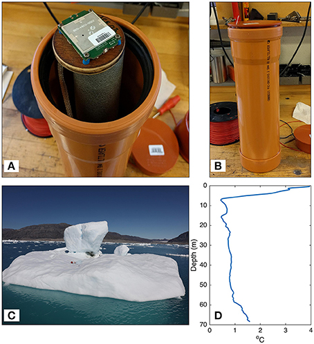
Figure 2. (A) An EXITE tracker showing Spot Trace GPS antenna mounting in a section of PVC drain pipe. (B) An assembled EXITE tracker. (C) EXITE on bergy bit with complex sail geometry resulting from ice debris. (D) A CTD profile of temperature with depth obtained in the vicinity of the EXITE deployment location.

The EXITE beacons were designed to be buoyant, given the short lifetime expectancies on the iceberg as mentioned above. After becoming dislodged from the iceberg or bergy bit, the EXITE beacon would transition from an iceberg tracker to a surface drifter to provide information about meltwater pathways. We planned to identify this transition using observed changes in velocity and/or acceleration, as will be described in detail below. An additional 1.2 kg of ballast was added in the form of scrap metal to the bottom of the PVC pipe. With the battery installed on top of the ballast the EXITE beacon floated nearly vertically with approximately 10 cm of pipe exposed to the air to provide the GPS with a clear view to the sky.

For the cylindrical housing and tag line, the slip speed is estimated following Suara et al. (2015) and references therein

$\begin{array}{cc}\left|U_s\right|=\frac{A}{R}{U}_a& \left(1\right)\end{array}$

where |U_s|, R, and U_a correspond to the slip velocity, ratio of drag on submerged to exposed area, and U_a is the wind speed, respectively. A = 0.07 (Niiler and Paduan, 1995). For the EXITE beacon, R = 6.4 and for wind speeds U_a in the range of 1–10 ms⁻¹ the slip velocity varies from 0.011 ms⁻¹ − 0.11 ms⁻¹. The implications of the larger slip speeds at higher wind speeds is addressed in Section 4. Velocity and acceleration metrics based on dynamic relations presented in Section 2.4 aid in the detection of the transition from ice to surface waters (see Section 2.5).

2.2. Field Study in Godthåbsfjord

Godthåbsfjord (GF) is a long (180 km), narrow (5 km), and deep (400–800 m) sill fjord in southwestern Greenland near Nuuk (Figure 1). During the summer, the fjord is influenced by meltwater and glacial ice input originating from the Greenland Ice Sheet. GF is in contact with three tidal outlet glaciers: Narssap Sermia (NS), Akugdlerssûp Sermia (AS), and Kangiata Nunâta Sermia (KNS) (Mortensen et al., 2011). GF receives runoff from three land-terminating glaciers, of which the largest drains through Lake Tasersuaq (LT; Figure 1). Turbid, freshwater inflow from the glaciers strongly impacts the surface circulation in GF during the summer melt water season (Mortensen et al., 2014). The seasonal water mass formation and resulting changes in circulation have been documented, but trajectories of individual icebergs and bergy bits have yet to be studied in GF.

7 EXITE beacons were thrown by hand into depressions and/or grooves on bergy bits near KNS on 8 August 2016 (Figures 1, 2C). Bergy bits are typically calved from a larger parent iceberg (Savage et al., 2000). However, the bergy bit classification used here is based only on estimated lengths of the tagged ice. The presence of smaller ice debris on the surfaces of the bergy bits suggests that they recently calved from KNS and were not produced by the breakup of larger icebergs. Though calving from KNS was not directly observed prior to tagging, icebergs (i.e., glacial ice with scales larger than those of bergy bits) are not observed in this area. The EXITE beacons were deployed within 1.3 km of each other over a span of 28 min (Figure 1). The tight spacing and short deployment time justifies the reasonable assumption that the tagged bergy bits were subject to the same initial forcing conditions. Furthermore, we can assume that, at least for a short time after deployment, any observed dispersion is due to either to differences in keel and sail geometries, submesoscale variability in ocean currents, or a combination of the two. 2 EXITE beacons were recovered by local hunters, thereby reducing their time in the field. Their retrieval, while unplanned, allowed us to assess their condition approximately 2 weeks after deployment. Additionally, the hunters were able to confirm that the beacons were drifting in the water at the time of retrieval. An attempt to retrieve several EXITE beacons during a routine monitoring cruise on 24 August 2016 proved unsuccessful due to high concentrations of small ice pieces (growlers and smaller) surrounding the beacons.

2.3. Supporting Data

Temperature profiles (Figure 2D) were collected with a CastAway conductivity, temperature, and depth probe (CTD) from a small work boat from the Greenland Institute of Natural Resources (GINR) in Nuuk. A meteorological station maintained by Asiaq Greenland Survey and located mid-fjord (Figure 1B) recorded air temperature, relative humidity, and wind speed during the study (Figures 3A–D). Unfortunately the meteorological station did not record wind direction. While wind speeds were relatively weak during the study period, two events with wind speeds >10 ms⁻¹ were observed. The timing of the stronger wind events coincided with flow reversals in the EXITE trajectories. To provide some indication of wind direction and, therefore, the possible role of winds in the flow reversal, large-scale winds over the study area are examined using 6 h reanalysis winds from the National Center for Environmental Prediction (NCEP)/National Center for Atmospheric Research (NCAR). Given the complex fjord geometry and orography it is unlikely that the coarse resolution reanalysis winds accurately resolved surface wind forcing in the fjord. 10 m resolution imagery of the GF region acquired by the Sentinel-2 satellite during the EXITE study is used to relate observed trajectories to ice concentrations and turbid melt water plumes. Unfortunately, the bergy bits tagged in this study were too small to be detected by the 10 m resolution Sentinel-2 imagery. Surface gravity wave amplitude was small in the inner fjord, likely due to the dampening effect of the ice as also observed and modeled by Ardhuin et al. (2011). A CTD transect obtained 8 August 2016 along the length of GF reveals large variations temperature, salinity, and density in the upper 15 m (Figures 3E,F) and the spatial variability in temperature suggests that melt rates due to basal melting and forced convection will vary with location in the fjord.

FIGURE 3

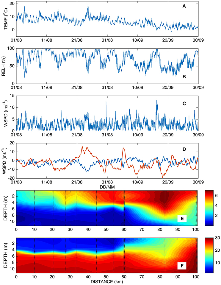
Figure 3. Time series of (A) air temperature, (B) relative humidity, and (C) wind speed during August and September 2016 as observed by the Asiaq Greenland Survey meteorological station. (D) Zonal (blue) and meridional (red) wind speeds from the NCEP/NCAR reanalysis grid point nearest GF. (E) Along-fjord transect of temperature and (F) salinity.

2.4. Bergy Bit Dynamics and Thermodynamics

Estimates of iceberg mass and surface area at the time of tagging are necessary to understand velocities and accelerations computed from EXITE trajectories. Most methods to estimate iceberg keel depth, volume, and mass require a priori knowledge of the waterline length. Dimensional analysis and curve fitting techniques have been employed to obtain desired unknown quantities (Savage et al., 2001) based on waterline length. However, the empirical relationships employed here were generated for bergy bits and icebergs with length scales greater than those of the bergy bits tagged in the present study. Furthermore, some empirical relationships exhibit divergent behavior at the extreme ends of the scales considered (e.g., Barker et al., 2004), calling their validity into question in the context of the present study. When possible, we draw upon studies of bergy bits (Dowdeswell and Forsberg, 1992; Savage et al., 2000, 2001; Ralph et al., 2008), however, melt rates obtained in open-ocean and laboratory environments may differ significantly from melt rates in GF where a warm, ≈ 10 m deep, layer develops in summer (Figures 3E,F).

Following Ralph et al. (2008), ice mass m can be computed

$\begin{array}{cc}m=(\frac{{\rho }_i{\rho }_w}{{\rho }_w-{\rho }_i})V_a& \left(2\right)\end{array}$

where ρ and V_a correspond to density and above-water volume, respectively. Subscripts i and w denote ice and water, respectively. Above water volume can be estimated following

$\begin{array}{cc}{V}_a=7.12LWHf& \left(3\right)\end{array}$

where L, W, H, and f correspond to above-water length, width, height and a shape-dependent scale factor (Ralph et al., 2008).

Savage et al. (2001) estimated iceberg volume using

$\begin{array}{cc}V=\kappa L^3& \left(4\right)\end{array}$

where κ = 0.45. Equation (4) can then be used to estimate mass by multiplying by ice density.

An iceberg of mass m drifts according to net force determined by the following equation

$\begin{array}{cc}m\frac{d{\overrightarrow{v}}_i}{dt}=-mf\overrightarrow{k}\times {\overrightarrow{v}}_i+{\overrightarrow{F}}_a+{\overrightarrow{F}}_w+{\overrightarrow{F}}_r+{\overrightarrow{F}}_s+{\overrightarrow{F}}_p& \left(5\right)\end{array}$

where ${\overrightarrow{v}}_i$, dt, f, $\overrightarrow{k}$ correspond to the iceberg velocity, time rate of change, Coriolis, and the vertical unit vector, respectively (Smith, 1993; Bigg et al., 1996, 1997). $\overrightarrow{F}$ corresponds to a given force and the subscripts a, w, r, s, and p denote forces due to air drag, water drag, wave radiation, sea ice drag, and horizontal pressure gradient, respectively. Following the treatment by FitzMaurice et al. (2016), the Coriolis force, wave radiation force, sea ice drag, and horizontal pressure gradient force can be neglected. In the data presented here, GF was free of sea ice and waves were small. Finally, the bergy bits were too small to exhibit significant horizontal pressure gradient forces or added mass. Under the aforementioned assumptions, Equation (5) reduces to

$\begin{array}{cc}m\frac{d{\overrightarrow{v}}_i}{dt}={\overrightarrow{F}}_a+{\overrightarrow{F}}_w& \left(6\right)\end{array}$

where

$\begin{array}{cc}{\overrightarrow{F}}_a=\frac{1}{2}{\rho }_a{C}_a{A}_a\left|{\overrightarrow{u}}_a-{\overrightarrow{v}}_i\right|({\overrightarrow{u}}_a-{\overrightarrow{v}}_i)& \left(7\right)\end{array}$

and

$\begin{array}{cc}{\overrightarrow{F}}_w=\frac{1}{2}{\rho }_w{C}_w{A}_w\left|{\overrightarrow{u}}_w-{\overrightarrow{v}}_i\right|({\overrightarrow{u}}_w-{\overrightarrow{v}}_i)& \left(8\right)\end{array}$

In Equations (7) and (8) ρ, C, A, and u correspond to fluid density, non-dimensional drag coefficient, cross-sectional area, and fluid velocity, respectively. The subscripts a and w denote air and water, respectively. Following FitzMaurice et al. (2016), C_a = 1.3 and C_w = 0.9. Equation (8) assumes a constant velocity over the keel. While shear was shown to be significant in modeling speeds of larger icebergs with deep (100–400 m) keel depths (FitzMaurice et al., 2016), its effect is likely less pronounced for the smaller, shallow-keeled bergy bits studied here (Dowdeswell and Forsberg, 1992).

Icebergs and bergy bits calved from the Greenland Ice Sheet are typically smaller and irregularly shaped when compared to their large tabular Antarctic counterparts (Bigg, 2016). The stability of tagged bergy bits can be evaluated using the Weeks-Mellor criterion (Bigg, 2016)

$\begin{array}{cc}\frac{L}{Z}<\sqrt{0.92+\frac{58.32}{Z}}& \left(9\right)\end{array}$

where L and Z correspond to the length and keel depth of the iceberg, respectively.

Ice mass and, by extension, volume and cross-sectional area vary over time, both gradually due to melting (Bigg et al., 1997), and episodically due to calving events (Savage et al., 2001). Most melt occurs below water in response to a combination of thermodynamic processes and the dominant processes affecting bergy bits in Godthåbsfjord are summarized here. For a complete treatment, see Bigg (2016). Despite the relatively warm observed air temperatures during the study period (Figure 3A), surface melt due to atmospheric fluxes was likely negligible compared to subsurface melt (Huppert, 1980). Sublimation was probably negligible due to prevailing humid conditions (Figure 3B).

The observed temperature profile (Figure 2D) and empirical relationships for basal and convective melt (Bigg, 2016) suggest depth-dependent melt rates. Warm surface waters (2–4°C) in the upper 10 m likely resulted in significant melting due to forced convection (Dowdeswell and Forsberg, 1992) and make fragmentation due to the footloose mechanism highly likely (Wagner et al., 2014). Likewise, water temperatures of approximately 1°C from 10 m down to the keel depth of the bergy bits likely drove appreciable basal melt. Using the empirical relationships for basal and convective melt summarized in Bigg (2016), the observed temperature profile, and assuming an average keel depth of 30 m, we estimate depth-integrated melt rates above and below 10 m to be >1 m day⁻¹ and 0.2 m day⁻¹, respectively, in the inner fjord.

Savage et al. (2001) estimated the melt rate of bergy bits due to wave erosion as

$\begin{array}{cc}L={\left[L_i^{5/4}-\zeta \Delta t\right]}^{4/5}& \left(10\right)\end{array}$

where L_i and Δt are the initial length of the bergy bit and a time interval, respectively, and

$\begin{array}{cc}\zeta =\frac{5\alpha }{12\kappa {\rho }_i}& \left(11\right)\end{array}$

In Equation (11) κ is the inverse of the aspect ratio and is set to 0.45 (Savage et al., 2000, 2001). ρ_i is the density of ice and

$\begin{array}{cc}\alpha =\beta \frac{k_w\Delta TH}{\Gamma }{\left[\frac{H^2}{\tau \nu }\right]}^{c_1}{\left[\frac{H}{g{\tau }^2}\right]}^{c_2}{\left[\frac{{\kappa }^{1/3}}{H}\right]}^{c_3}& \left(12\right)\end{array}$

In Equation (12), k_w, ΔT, H, τ, Γ, ν, and g correspond to the thermal conductivity of seawater, water/melting ice temperature difference, wave height, wave period, latent heat of fusion, kinematic viscosity of seawater, and acceleration due to gravity, respectively. β, c₁, c₂, and c₃ are constants determined through fitting curves to observed bergy bit melt rates (Savage et al., 2001). Equations 10–12 do not account for temporal variability of parameters such as wave height and, therefore, is valid only for a sufficiently short period of time (e.g., Δt ≈ 1 day).

Wave erosion has been suggested as the dominant process responsible for iceberg mass loss (Huppert, 1980; Savage et al., 2001). In the inner fjord, where ice abundance is high, waves are small due to limited fetch and the dampening effect of the ice. Quantitative wave measurements are lacking in GF, but qualitative visual observations by the authors suggest small waves with high frequencies in the inner part of the fjord. Using H = 0.25 m, τ = 1 s, ΔT = 2°C, and L_i = 20 m, results in a melt rate > 2 m day⁻¹. Combined with forced convection and basal melt, the expected lifetime of bergy bits tracked in this study is approximately 10 days.

2.5. Data Analysis

Observed positions in degrees of latitude and longitude were converted to universal transverse Mercator (UTM) easting ($\overrightarrow{X}$) and northing ($\overrightarrow{Y}$) coordinates. The nominal period between observations was 5 min but gaps were common and were most likely due to poor antenna orientation. Gaps of 20 min or less were common with a few longer gaps of approximately 6 h. Additionally, spurious positions, most likely due to multi-path transmission errors, were also present in the data that could result in erroneously large accelerations. While obvious position errors could be identified by plotting the trajectories (i.e., positions that “jumped” onto land) the more subtle spurious positions were identified by computing a 12 h moving average of displacements with 50% overlap. Displacements larger than the mean plus 2 standard deviations were rejected. Hourly average positions were computed from the resulting dataset. Zonal ($\overrightarrow{u}$) and meridional ($\overrightarrow{v}$) velocities and accelerations were calculated from hourly average UTM positions using a central difference scheme.

Length along the waterline, average height above the waterline, and above-water surface area were estimated from photographs taken during deployment. A 50.6 megapixel Canon 5DSR Mk. III full-frame DSLR camera equipped with a 24 mm lens was used to photograph bergy bits. Lens distortion was corrected using the Camera Calibration Toolbox for Matlab (http://www.vision.caltech.edu/bouguetj/calib_doc/). When possible, the undistorted images were binarized, thresholded, and segmented to create a mask that was then used to extract relevant dimensions in pixels. Pixel measurements were converted to their dimensional equivalents using the EXITE tracker for a reference scale. Thus, the dimensions are estimated to aid in assigning an appropriate size classification and in analyses of observed velocities and accelerations. Keel depths, volume, and mass were estimated using the dimensional analyses of Ralph et al. (2008), Barker et al. (2004), and Savage et al. (2001).

Using the maximum observed EXITE velocities and wind speeds we can estimate the forces due to air and water friction using Equations (7) and (8) using the dimensional estimates for each iceberg (Table 1). Wind speeds in the study area were relatively weak, with a mean of 2.8 ms⁻¹ for the entire period (Figure 3C). Given the relatively small iceberg velocities observed by the EXITE trackers, we approximate ${\overrightarrow{u}}_a-{\overrightarrow{v}}_i$ as ${\overrightarrow{u}}_a$ in Equation (7). Unfortunately we do not have the concurrent observations of ocean currents to estimate the relative velocity between ice and ocean in Equation (8). However, given that iceberg velocities are comparable to upper ocean velocities observed by Mortensen et al. (2014) and given that numerous previous studies found ocean currents to be the dominant force behind iceberg motion, we assume that this relative velocity is ≤ 0.05 ms⁻¹. The upper limit for acceleration for each bergy bit is then estimated by dividing the total force ${\overrightarrow{F}}_t={\overrightarrow{F}}_a+{\overrightarrow{F}}_w$ by the estimates of mass at the time of tagging. This critical acceleration is then used to aid in determining when a given EXITE beacon transitions to a surface drifter.

TABLE 1

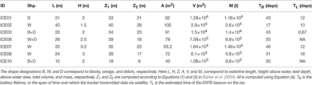
Table 1. Shape and estimated dimensions of icebergs tagged with EXITE beacons.

3. Results

The EXITE beacons exceeded expectations, with 5 of the 7 meeting or exceeding the 30 day battery life requirement (Table 1). Data transmission gaps were typically small (see Section 2.5), with the exception of a 15 day gap for one beacon. The waterline length of the tagged icebergs ranged from 15 to 40 m (Table 1). The lengths of the tagged ice masses placed them in the bergy bit size category. However, we stress that the bergy bits studied here were mostly likely recently calved from their parent glacier, and not the result of fragmentation of a larger iceberg. Estimated keel depths ranged from 9 to 40 m and the subsurface warming observed in the temperature profile suggests a maximum keel depth of ice in the region of <60 m (Figure 2D). All tagged icebergs were between 1 and 3 m in height above the waterline, though the height of some of the debris reached up to 5 m. Initial ice mass ranged from 1 × 10³ tons to 2.9 × 10⁴ tons (Table 1). Based on the estimated waterline lengths and keel depths, and using Equation (9), the bergy bits were most likely unstable when tagged. Assuming a conservative melt rate of 2 m day⁻¹ the lifetime of the bergy bits tagged in this study ranges from 7.5 to 20 days.

The trackers reveal complex bergy bit and surface water transport with evidence of the influence of topographic eddies, collisions with fjord walls, freshwater outflows, and a large flow reversal (Figures 4–10). Observed velocities were generally weak (≈0.1 ms⁻¹), though short bursts up to 0.6 ms⁻¹ were recorded (Figure 11). Typical accelerations observed by a drifting EXITE beacon were ≈10⁻⁵ms⁻² (Figure 12). Collisions with fjord walls shown by EXITE trajectories (Figures 4–10) exhibit corresponding spikes in acceleration up to an order of magnitude larger.

FIGURE 4

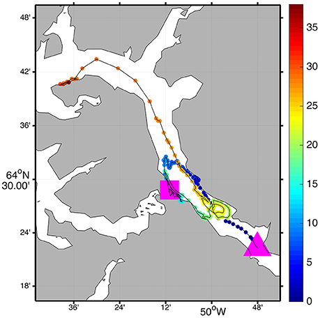
Figure 4. A trajectory of an EXITE beacon initially deployed at the large pink triangle. Locations are color-coded according to time, in days, since deployment. Every 4th measurement is shown for clarity. The location where the critical acceleration was exceeded is indicated by the large pink square.

FIGURE 5

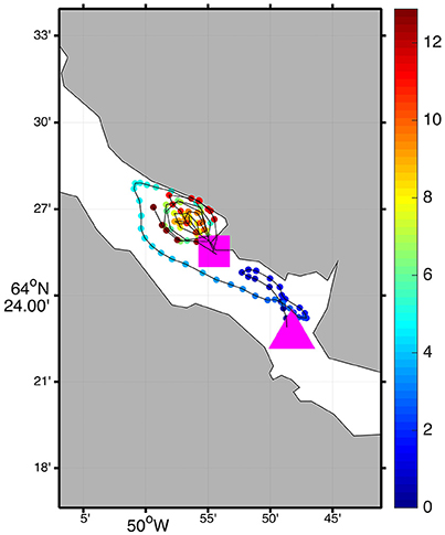
Figure 5. A trajectory of an EXITE beacon initially deployed at the large pink triangle. Locations are color-coded according to time, in days, since deployment. Every 4th measurement is shown for clarity. The location where the critical acceleration was exceeded is indicated by the large pink square.

FIGURE 6

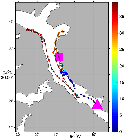
Figure 6. A trajectory of an EXITE beacon initially deployed at the large pink triangle. Locations are color-coded according to time, in days, since deployment. Every 4th measurement is shown for clarity. The location where the critical acceleration was exceeded is indicated by the large pink square.

FIGURE 7

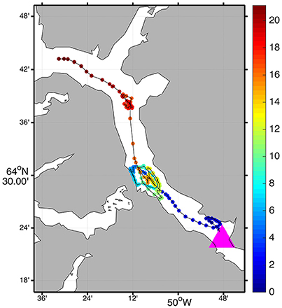
Figure 7. A trajectory of an EXITE beacon initially deployed at the large pink triangle. Locations are color-coded according to time, in days, since deployment. Every 4th measurement is shown for clarity.

FIGURE 8

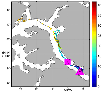
Figure 8. A trajectory of an EXITE beacon initially deployed at the large pink triangle. Locations are color-coded according to time, in days, since deployment. Every 4th measurement is shown for clarity. The location where the critical acceleration was exceeded is indicated by the large pink square.

FIGURE 9

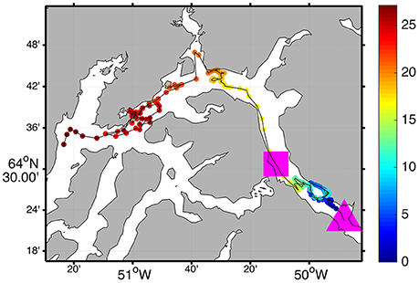
Figure 9. A trajectory of an EXITE beacon initially deployed at the large pink triangle. Locations are color-coded according to time, in days, since deployment. Every 4th measurement is shown for clarity. The location where the critical acceleration was exceeded is indicated by the large pink square.

FIGURE 10

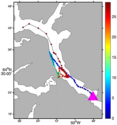
Figure 10. A trajectory of an EXITE beacon initially deployed at the large pink triangle. Locations are color-coded according to time, in days, since deployment. Every 4th measurement is shown for clarity.

FIGURE 11

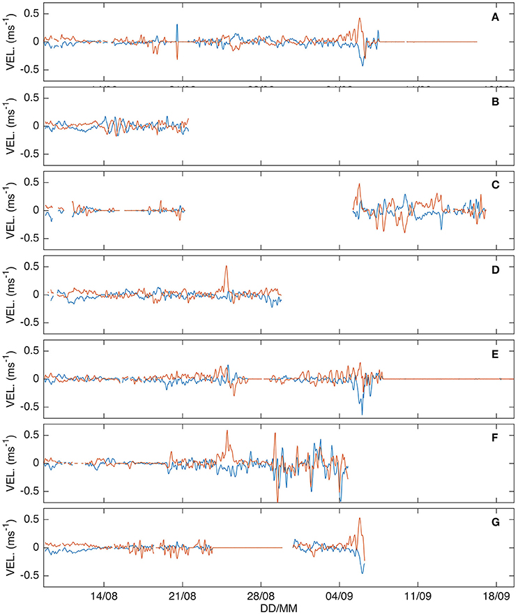
Figure 11. Zonal (blue) and meridional (red) velocity components for each EXITE beacon.

FIGURE 12

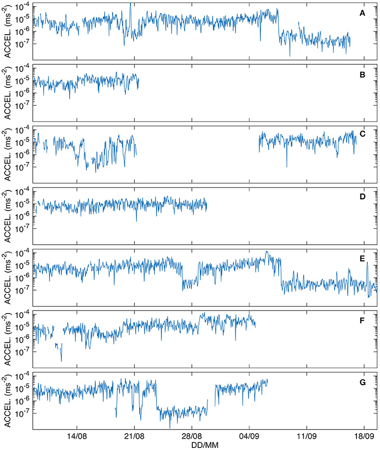
Figure 12. Magnitude of acceleration for each EXITE beacon during August–September 2016.

In general, most EXITE beacons exceeded their respective critical accelerations during collisions with fjord walls. The estimated transition point in each EXITE trajectory is indicated by a pink square, when applicable, in Figures 4–10. Estimated time of an EXITE beacon on a bergy bit ranged from less than 1 day to up to 16 days (Table 1). The critical acceleration metric failed for 2 EXITE beacons that exhibited small accelerations in general and no detectable spikes (Figures 12D,G). In general, the observed speeds increased after the critical accelerations were exceeded. This observed increase in speed likely corresponds to the added slip velocity (Equation 1) that results from wind acting on the exposed portion of the drifting EXITE beacon.

Two beacons were transported to within a few km of the calving front of NS (Figures 6, 8). Upon reaching NS, both beacons reversed course and one was transported back to within 8 km of its deployment location (Figure 6). These reversals were likely due to winds up to 10 ms⁻¹ observed on 8–9 September (Figure 3C). Unfortunately the local meteorological station (Figure 1) did not record wind direction, but the southward reversal and the fact that a third beacon was driven into the southern wall of the fjord (opposite the LT outflow) by the same wind event (Figure 4) suggests that the wind had a strong northerly component. NCEP/NCAR reanalysis winds from the grid point nearest GF show strong northerly winds during this time (Figure 3D). The Sentinel-2 image from 10 September 2016 shows evidence of surface flow toward KNS in turbidity and ice accumulation in small indentations in south/west coast (Figure 13).

FIGURE 13

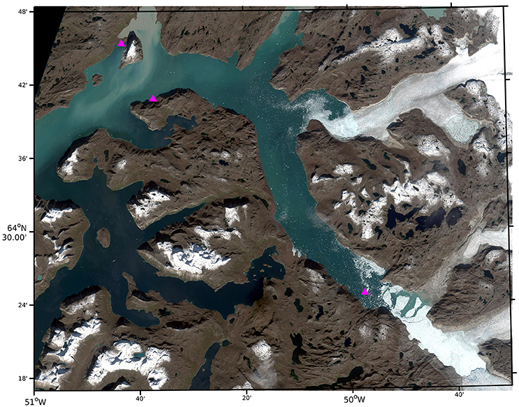
Figure 13. Contrast-enhanced, color image of the inner Godthåbsfjord region acquired 10 September 2016. The positions of the 3 active EXITE beacons at the time of acquisition are shown by pink triangles.

Additional evidence of the complexity of surface transport in GF comes from a tracker that traveled upstream into the LT outflow (Figure 9). The upstream incursion that began around 29 August did not coincide with an increase in wind speed (Figure 3C) and was likely due to variability in strength of the outflow. The shallow (5 m) depths in the LT outflow suggests that this specific beacon was acting as a surface drifter. Sentinel-2 imagery of the area during the EXITE study shows considerable variability in the extent and shape of the LT outflow, with many small-scale fronts and eddies visible.

4. Discussion

The EXITE beacons successfully tracked bergy bits and melt water in their first deployment in GF at a fraction of the cost of commercially available drifters and ice trackers. In addition to tracking general out-fjord transport of solid and liquid freshwater, the EXITE trajectories reveal complexity in the shallow circulation in the form of small-scale eddies and wind-driven reversals. One such reversal transported an EXITE tracker to within 8 km of its original deployment location. The differences in dispersion between initially proximal bergy bits highlight the importance of small-scale variability in ocean currents and the chaotic, unpredictable nature of Lagrangian transport. The importance of and interplay between winds and freshwater plumes is also apparent when the EXITE trajectories are compared to high-resolution satellite imagery.

The observed velocities agree well with previous studies of icebergs in both open water (Smith, 1993) and other fjords in Greenland (Sutherland et al., 2014; Andres et al., 2015). The looping behavior observed is similar to those observed by Sutherland et al. (2014). However, the dimensional relationships used to estimate bergy bit keel depths and mass (Table 1) are based on limited number observations. For example, the smallest iceberg used by Barker et al. (2004) to estimate masses was 50 m in length. For comparison, the largest bergy bit studied here was 40 m in length. Additionally, the presence of debris resulted in complex bergy bit sail geometries (Figure 2C) that were not accounted for in the simplistic estimates of sail area. Similarly, the expressions for iceberg melt rates were also obtained using either data collected in open water or in laboratory tests that attempted to replicate open water conditions (Bigg, 2016).

Empirical relationships for basal and convective melt also need to be verified for icebergs and bergy bits in a fjord setting. The combined lateral and vertical temperature stratification observed in Godthåbsfjord in August 2016 likely resulted in both depth and spatially dependent melt rates (Figures 3E,F). Near the mélanges, the high concentration of ice is likely responsible for the large temperature gradient observed below 10 m (Figure 2D). Subsurface melt rates will likely increase away from the insulating effect of the mélanges. Convective melt rates depend on the relative velocity between ice and water (Bigg, 2016). Thus, observations of velocity and velocity shear around icebergs and bergy bits will also help constrain melt rates.

While a wide range of size classes of ice can be tracked by radar and time lapse imagery (Turnbull et al., 2015; Voytenko et al., 2015) observed trajectories will be limited to the footprint of the radar or camera. Additionally, radar observations require either a dedicated ship or a land station with adequate power and infrastructure. Satellite and aerial remote sensing techniques can provide valuable size and concentration data. However, irregularly shaped icebergs of Greenlandic origin are prone to rolling making identification and tracking of individual icebergs challenging.

The application of historical scaling relationships highlights the need for additional measurements of ice over a wider range of size scales. Understanding of bergy bit drift and deterioration will require comprehensive measurements of both ice geometry and ambient fjord conditions. Ideally, such a comprehensive study would include tagging of drifting icebergs and bergy bits in a region instrumented with acoustic Doppler current profilers (ADCP), CTDs, and weather stations. Time lapse cameras and/or radar would also provide insight into the motion of all the ice in the field of view.

While the EXITE beacons provided the first observations of bergy bit transport in GF, the biggest drawback of the present design is the uncertainty in timing of transition from an ice tracker to a surface drifter. The critical acceleration metric devised to estimate the time of transition relies on dated scaling relationships that were largely developed for larger pieces of ice and in an open ocean setting. The initial mass estimates are, therefore, subject to error, the magnitude of which is difficult estimate given the multiple sources of uncertainty. The critical acceleration metric also uses an estimate of ice mass at the time of tagging and does not take changes in mass due to melting and fragmentation into account. In most cases, the critical acceleration is exceeded when an EXITE beacon decelerates rapidly during a collision with a fjord wall. Given that all of the bergy bits satisfied the criterion for instability (Equation 9) when initially tagged, it comes as no surprise that the bergy bit could capsize during a collision with a solid boundary. Improvements to the existing design are discussed in Section 4.1.

The initial mass used to estimate the critical acceleration also changes in time due to the relatively high (estimated) melt rate. A melt rate of 1.2 m day⁻¹ corresponds to a decrease in ice mass of approximately 700 kg day⁻¹. The highest melt rates will result from wave erosion and, in the absence of waves, the warm (4–5°C) surface (0–10 m) layer will lead to similar melt rates. Both processes result in the undercutting observed below the waterlines of several of the bergy bits tagged in this study (Figure 2D), which can result in complex keel geometries that were not encountered in open-water (Ralph et al., 2008) and laboratory studies (Savage et al., 2001) of ice melt. The depth-dependent melt rate likely leads to gradual tilting of bergy bits and icebergs as suggested by the remnants of multiple waterlines visible on ice in GF and fragmentation due to the footloose mechanism. Given that the lifetime of a 20 m-long bergy bit subject to an average melt rate of 2 m day⁻¹ is 10 days, the estimated times on the ice of the EXITE beacons are fairly reasonable (Table 1).

The recovery of 2 EXITE beacons provided first-hand verification of their drifting status. A dedicated attempt to recover 2 EXITE beacons on 24 August was unsuccessful due to the large amount of growlers and smaller ice fragments in the vicinity of the positions reported by the beacons. The Sentinel-2 image from the same day (not shown) verifies these conditions. The trapping of EXITE beacons in a high concentration of small pieces of ice may have limited their ability to drift freely and, as a result, their observed accelerations likely reflect the collective response, or added mass, of the ice and surface water. In other words, the net effect of many small pieces of ice concentrated in a small area may be to resemble the drift of a larger, single piece of ice. The coherent patches of small ice fragments visible in the Sentinel-2 imagery may result from geostrophic adjustment, especially toward the mouth of the fjord where the density gradients between the localized melt water and ambient water are larger.

A wind-related metric was also devised in an attempt to detect the transition from an ice tracker to a surface drifter. As surface currents typically respond nearly instantaneously to wind forcing (Ursella et al., 2006), the speed of a beacon floating in the water should correlate with local wind speed. To test this possible detection metric, the cross-correlations of 60 h segments of EXITE velocities and wind speeds observed at the Asiaq meteorological station (Figure 2B). However, the EXITE beacons spent much of their lifetimes in the inner fjord where winds could have differed significantly from the observations at the meteorological station. Additionally, if drifting beacons were actually inside a coherent structure of ice fragments (growlers and smaller) and melt water, then their trajectories should differ from an unrestricted surface drifter.

Despite the complex problem of identifying the transition from iceberg tracker to surface drifter we decided that it was a worthwhile exercise to attempt. It is our hope that others will adopt the general design presented here and, should attempts to detect the transition from iceberg tracker to surface drifter fail, the EXITE beacon can be constructed such that it will sink once dislodged from the ice. Negative buoyancy can be achieved simply by increasing the ballast or decreasing the internal volume of the PVC housing, or by doing both. An instrumented tracker, currently under development, is described briefly below. When completed, it provide a more reliable estimate of the time of transition to a surface drifter using conductivity and temperature measurements, as well as observations of these variables along its trajectory.

4.1. Next Generation EXITE

While the EXITE prototype described here exceeded all expectations, the next generation of EXITE trackers has been modified slightly to extend battery life and improve reliability. Two versions are in development. The first version simply improves on the original design and incorporates a higher capacity, industrial-strength battery (6V, 27 Ah) that should result in significantly longer lifetimes. The battery and GPS are still housed in a section of PVC but the internal frame is now constructed out of laser-cut plywood. One-way vents have been installed in the cap to allow any gas buildup in the housing to escape. An optional external collar can be attached to the top of the tracker to provide the GPS antenna with a better view of the sky while on the ice. The second version in development takes advantage of open-source developments in the unmanned aerial systems (UAS) and remotely operated vehicles (ROV) sectors. This version incorporates more internal and external sensors to provide higher temporal resolution measurements of position, rotation, and acceleration, as well as temperature and conductivity. At first glance, EXITE is similar in construction to other low-cost drifters (Johnson et al., 2003; Larsen et al., 2015). The use of low-cost, OTS materials will result in some similarities in available waterproof housings. EXITE differs from other low-cost drifters in the number of components required, ease of construction, high frequency transmission of position data via satellite, and its application as an ice tracker. While there are certainly better surface drifters available to the scientific community, there are few affordable GPS-based ice trackers with high-frequency satellite communication available.

5. Conclusions

Understanding ice sheet-ocean interactions will require application of observations, models, and theory to the fjords where these two systems interact. While remote sensing techniques provide estimates of melt rates of ice in fjords (Enderlin et al., 2016) and the rate of retreat of marine-terminating glaciers, a gaping hole in understanding the fjord system is the lack of Lagrangian observations of transport of ice and melt water. Parameterizing the magnitude, location, and timing of these freshwater fluxes is critical in the development of accurate ocean and climate models. Furthermore, understanding the response of bergy bits to ocean and atmospheric forcing will aid in risk management in Greenlandic waters and enhance safety at sea. We developed the expendable ice tracker (EXITE) specifically to study Lagrangian transport of bergy bits and glacial melt water in Godthåbsfjord in southwest Greenland. Given a total cost of $300, simple, open-source design, and demonstrated ability we hope that the EXITE beacons will be deployed by research groups and citizen science initiatives in other Arctic regions.

Author Contributions

DC, WB, LM, SR, and JA contributed to experiment planning, data collection, and interpretation of results. DC designed and constructed the trackers, analyzed the data, and prepared the bulk of the manuscript.

Conflict of Interest Statement

The authors declare that the research was conducted in the absence of any commercial or financial relationships that could be construed as a potential conflict of interest.

Acknowledgments

Erling Pedersen assisted in the construction of the trackers and Egon Randa Frandsen, Emmelia Wiley, and Carl Isaksen assisted with logistics. Masayo Ogi assisted with deployment of the EXITE beacons and collection of other field data. Diego Mejia at Globalstar provided SPOT Trace units with custom firmware. We gratefully acknowledge the contributions of Arctic Research Centre (ARC), Aarhus University and by the Canada Excellence Research Chair (CERC). This work is a contribution to the Arctic Science Partnership (ASP) http://asp-net.org. The Greenland Research Council and the Greenland Ecosystem Monitoring Subprogram ClimateBasis are acknowledged, as well as Stefan Wacker for AWS management.

Abbreviations

EXITE, expendable ice tracker; GPS, global positioning system; LT, Lake Tasersuaq. Location in Godthåbsfjord (Figure 1B); GF, Godthåbsfjord.

References

Amundson, J. M., Fahnestock, M., Truffer, M., Brown, J., Luüthi, M. P., and Motyka, R. J. (2010). Ice mélange dynamics and implications for terminus stability, Jakobshavn Isbræ, Greenland. J. Geophys. Res. 115:F01005. doi: 10.1029/2009JF001405

CrossRef Full Text | Google Scholar

Andres, M., Silvano, A., Straneo, F., and Watts, D. (2015). Icebergs and sea ice detected with inverted echo sounders. J. Atmospher. Oceanic Technol. 32, 1042–1057. doi: 10.1175/JTECH-D-14-00161.1

CrossRef Full Text | Google Scholar

Ardhuin, F., Tournadre, J., Queffeulou, P., Girard-Ardhuin, F., and Collard, F. (2011). Observation and parameterization of small icebergs: drifting breakwaters in the southern ocean. Ocean Model. 39, 405–410. doi: 10.1016/j.ocemod.2011.03.004

CrossRef Full Text | Google Scholar

Barker, A., Sayed, M., and Carrieres, T. (2004). “Determination of iceberg draft, mass and cross-sectional areas,” in Proceedings of 14th International Offshore and Polar Engineering Conference (Toulon: International Society of Offshore and Polar Engineers), 899–904.

Google Scholar

Bigg, G. (2016). Icebergs: Their Science and Links to Global Change. Cambridge University Press. doi: 10.1017/CBO9781107589278

CrossRef Full Text

Bigg, G., Wadley, M., Stevens, D., and Johnson, J. (1996). Prediction of iceberg trajectories for the North Atlantic and Arctic Oceans. Geophys. Res. Lett. 23, 3587–3590. doi: 10.1029/96GL03369

CrossRef Full Text | Google Scholar

Bigg, G., Wadley, M., Stevens, D., and Johnson, J. (1997). Modelling the dynamics and thermodynamics of icebergs. Cold Regions Sci. Technol. 26, 113–135. doi: 10.1016/S0165-232X(97)00012-8

CrossRef Full Text | Google Scholar

Buus-Hinkler, J., Qvistgaard, K., and Krane, K. (2014). “Iceberg number density - reaching a full picture of the greenland waters,” in 2014 IEEE Geoscience and Remote Sensing Symposium (Québec: IEEE), 270–273. doi: 10.1109/IGARSS.2014.6946409

CrossRef Full Text | Google Scholar

Crocker, G., and Cammaert, G. (1994). “Measurements of bergy bit and growler populations off Canada's east coast,” in IAHR Ice Symposium (Trondheim), 167–176.

Crocker, G., and English, J. (1998). Verification and Implementation of a Methodology for Predicting Bergy Bit and Growler Populations. Tech. rep., Ice Services, Environment Canada.

Crocker, G., English, J., McKenna, R., and Gagnon, R. (2004). Evaluation of bergy bit populations on the Grand Banks. Cold Regions Sci. Technol. 38, 239–250. doi: 10.1016/j.coldregions.2003.12.001

CrossRef Full Text | Google Scholar

Death, R., Siegert, M., Bigg, G., and Wadley, M. (2006). Modelling iceberg trajectories, sedimentation rates and meltwater input to the ocean from the Eurasian Ice Sheet at the Last Glacial Maximum. Palaeogeogr. Palaeoclimatol. Palaeoecol.gy 236, 135–150. doi: 10.1016/j.palaeo.2005.11.040

CrossRef Full Text | Google Scholar

Dowdeswell, J., and Forsberg, C. (1992). The size and frequency of icebergs and bergy bits derived from tidewater glaciers in Kongsfjorden, northwest Spitsbergen. Polar Res. 11, 81–91. doi: 10.3402/polar.v11i2.6719

CrossRef Full Text | Google Scholar

Eik, K., and Gudmestad, O. (2010). Iceberg management and impact on design of offshore structures. Cold Regions Sci. Technol. 63, 15–28. doi: 10.1016/j.coldregions.2010.04.008

CrossRef Full Text | Google Scholar

Enderlin, E., and Hamilton, G. (2014). Estimates of iceberg submarine melting from high-resolution digital elevation models: application to Sermilik Fjord, East Greenland. J. Glaciol. 60, 1084–1092. doi: 10.3189/2014JoG14J085

CrossRef Full Text | Google Scholar

Enderlin, E., Hamilton, G., Straneo, F., and Sutherland, D. (2016). Iceberg meltwater fluxes dominate the freshwater budget in Greenlands iceberg-congested glacial fjords. Geophys. Res. Lett. 43, 11287–11294. doi: 10.1002/2016GL070718

CrossRef Full Text | Google Scholar

FitzMaurice, A., Straneo, F., Cenedese, C., and Andres, M. (2016). Effect of a sheared flow on iceberg motion and melting. Geophys. Res. Lett. 43, 12520–12527. doi: 10.1002/2016GL071602

CrossRef Full Text | Google Scholar

Gagnon, R. (2008). Analysis of data from bergy bit impacts using a novel hull-mounted external impact panel. Cold Regions Sci. Technol. 52, 50–66. doi: 10.1016/j.coldregions.2007.04.018

CrossRef Full Text | Google Scholar

Huppert, H. (1980). The physical processes involved in the melting of icebergs. Ann. Glaciol. 1, 97–101.

Google Scholar

Johnson, D., Stocker, R., Head, R., Imberger, J., and Pattiaratchi, C. (2003). A compact, low-cost GPS drifter for use in the oceanic nearshore zone, lakes, and estuaries. J. Atmospher. Ocean. Technol. 20, 1880–1884. doi: 10.1175/1520-0426(2003)020<1880:ACLGDF>2.0.CO;2

CrossRef Full Text | Google Scholar

Larsen, P.-H., Hansen, M. O., Buus-Hinkler, J., Krane, K. H., and Sønderskov, C. (2015). Field tracking (GPS) of ten icebergs in eastern Baffin Bay, offshore Upernavik, northwest Greenland. J. Glaciol. 61, 421–437. doi: 10.3189/2015JoG14J216

CrossRef Full Text | Google Scholar

Martin, T., and Adcroft, A. (2010). Parameterizing the fresh-water flux from land ice to ocean with interactive icebergs in a coupled climate model. Ocean Model. 34, 111–124. doi: 10.1016/j.ocemod.2010.05.001

CrossRef Full Text | Google Scholar

Mortensen, J., Bendtsen, J., Lennert, K., and Rysgaard, S. (2014). Seasonal variability of the circulation system in a west greenland tidewater outlet glacier fjord, Godthåbsfjord (64°N). J. Geophys. Res. Earth Surf. 119, 2591–2603. doi: 10.1002/2014JF003267

CrossRef Full Text | Google Scholar

Mortensen, J., Lennert, K., Bendtsen, J., and Rysgaard, S. (2011). Heat sources for glacial melt in a sub-Arctic fjord (Godthåbsfjord) in contact with the Greenland ice Sheet. J. Geophys. Res. 116:C01013. doi: 10.1029/2010JC006528

CrossRef Full Text | Google Scholar

Niiler, P., and Paduan, J. (1995). Wind-driven motions in the northeast Pacific as measured by Lagrangian drifters. J. Phys. Oceanogr. 25, 2819–2830. doi: 10.1175/1520-0485(1995)025<2819:WDMITN>2.0.CO;2

CrossRef Full Text | Google Scholar

Poje, A., Ozgokmen, T. M., Lipphardt, B. L. Jr., Haus, B., Haza, A., Jacobs, G., et al. (2014). Submesoscale dispersion in the vicinity of the Deepwater Horizon spill. Proc. Natl. Acad. Sci. U.S.A. 111, 12693–12698. doi: 10.1073/pnas.1402452111

PubMed Abstract | CrossRef Full Text | Google Scholar

Ralph, F., McKenna, R., and Gagnon, R. (2008). Iceberg characterization for the bergy bit impact study. Cold Regions Sci. Technol. 52, 7–28. doi: 10.1016/j.coldregions.2007.04.016

CrossRef Full Text | Google Scholar

Savage, S., Crocker, G., Sayed, M., and Carrieres, T. (2000). Size distributions of small ice pieces calved from icebergs. Cold Regions Sci. Technol. 31, 163–172. doi: 10.1016/S0165-232X(00)00010-0

CrossRef Full Text | Google Scholar

Savage, S., Crocker, G., Sayed, M., and Carrieres, T. (2001). Bergy bit and growler melt deterioration. J. Geophys. Res. 106, 11493–11504. doi: 10.1029/2000JC000270

CrossRef Full Text | Google Scholar

Smith, S. (1993). Hindcasting iceberg drift using current profiles and winds. Cold Regions Sci. Technol. 22, 33–45. doi: 10.1016/0165-232X(93)90044-9

CrossRef Full Text | Google Scholar

Suara, K., Wang, C., Feng, Y., Brown, R., Chanson, H., and Borgas, M. (2015). High-resolution GNSS-tracked drifter for studying surface dispersion in shallow water. J. Atmospher. Ocean. Technol. 32, 579–590. doi: 10.1175/JTECH-D-14-00127.1

CrossRef Full Text | Google Scholar

Sulak, D., Sutherland, D., Enderlin, E., Stearns, L., and Hamilton, G. (2017). Iceberg properties and distributions in three Greenlandic fjords using satellite imagery. Ann. Glaciol. doi: 10.1017/aog.2017.5 Available online at: https://www.cambridge.org/core/journals/annals-of-glaciology/article/iceberg-properties-and-distributions-in-three-greenlandic-fjords-using-satellite-imagery/A9696493A23345C13DD36E378300A264#

CrossRef Full Text | Google Scholar

Sutherland, D., Roth, G., Hamilton, G., Mernild, S., Stearns, L., and Straneo, F. (2014). Quantifying flow regimes in a Greenland glacial fjord using iceberg drifters. Geophys. Res. Lett. 41, 8411–8420. doi: 10.1002/2014GL062256

CrossRef Full Text | Google Scholar

Turnbull, I., Fournier, N., Stolwijk, M., Fosnaes, T., and McGonigal, D. (2015). Operational iceberg drift forecasting in Northwest Greenland. Cold Regions Sci. Technol. 110, 1–18. doi: 10.1016/j.coldregions.2014.10.006

CrossRef Full Text | Google Scholar

Ursella, L., Poulain, P.-M., and Signell, R. P. (2006). Surface drifter derived circulation in the northern and middle Adriatic Sea: response to wind regime and season. J. Geophys. Res. 111:C03S04. doi: 10.1029/2005jc003177

CrossRef Full Text | Google Scholar

Voytenko, D., Dixon, T., Luther, M., Lembke, C., Howat, I., and de la Pena, S. (2015). Observations of inertial currents in a lagoon in southeastern Iceland using terrestrial radar interferometry and automated iceberg tracking. Comput. Geosci. 82, 23–30. doi: 10.1016/j.cageo.2015.05.012

CrossRef Full Text | Google Scholar

Wagner, T., Wadhams, P., Bates, R., Elosegui, P., Stern, A., Vella, D., et al. (2014). The “footloose” mechanism: iceberg decay from hydrostatic stresses. Geophys. Res. Lett. 41, 5522–5529. doi: 10.1002/2014GL060832

CrossRef Full Text | Google Scholar