Comparing Apples to Oranges: Common Trends and Thresholds in Anthropogenic and Environmental Pressures across Multiple Marine Ecosystems
 Jamie C. Tam1*†
  Jason S. Link1
  Scott I. Large2
  Kelly Andrews3
  Kevin D. Friedland4 Jamison Gove5 Elliott Hazen6 Kirstin Holsman7 Mandy Karnauskas8
  Jameal F. Samhouri3
  Rebecca Shuford9 Nick Tomilieri3 Stephani Zador7
- 1NOAA Fisheries, National Marine Fisheries Service, Woods Hole, MA, United States
- 2International Council for the Exploration of the Seas, Copenhagen, Denmark
- 3NOAA Fisheries, Northwest Fisheries Science Center, Seattle, WA, United States
- 4NOAA Fisheries, Northeast Fisheries Science Center, Narragansett, RI, United States
- 5NOAA Fisheries, Pacific Island Fisheries Science Center, Honolulu, HI, United States
- 6NOAA Fisheries, Southwest Fisheries Science Center, Monterey Bay, CA, United States
- 7NOAA Fisheries, Alaska Fisheries Science Center, Seattle, WA, United States
- 8NOAA Fisheries, Southeast Fisheries Science Center, Miami, FL, United States
- 9NOAA Fisheries, Office of Science and Technology, Silver Spring, MD, United States
Ecosystem-based management (EBM) in marine ecosystems considers impacts caused by complex interactions between environmental and anthropogenic pressures (i.e., oceanographic, climatic, socio-economic) and marine communities. EBM depends, in part, on ecological indicators that facilitate understanding of inherent properties and the dynamics of pressures within marine communities. Thresholds of ecological indicators delineate ecosystem status because they represent points at which a small increase in one or many pressure variables results in an abrupt change of ecosystem responses. The difficulty in developing appropriate thresholds and reference points for EBM lies in the multidimensionality of both the ecosystem responses and the pressures impacting the ecosystem. Here, we develop thresholds using gradient forest for a suite of ecological indicators in response to multiple pressures that convey ecosystem status for large marine ecosystems from the US Pacific, Atlantic, sub-Arctic, and Gulf of Mexico. We detected these thresholds of ecological indicators based on multiple pressures. Commercial fisheries landings above approximately 2–4.5 t km−2 and fisheries exploitation above 20–40% of the total estimated biomass (of invertebrates and fish) of the ecosystem resulted in a change in the direction of ecosystem structure and functioning in the ecosystems examined. Our comparative findings reveal common trends in ecosystem thresholds along pressure gradients and also indicate that thresholds of ecological indicators are useful tools for comparing the impacts of environmental and anthropogenic pressures across multiple ecosystems. These critical points can be used to inform the development of EBM decision criteria.
Introduction
Ecosystem-based management (EBM) of the ocean, which considers the management of the broad range of ecosystem services across ocean-use sectors (Slocombe, 1993; Leslie and McLeod, 2007), is designed to balance the needs of society for utilization of ecosystem services (e.g., living marine resources) with the sustainability and conservation of marine ecosystems. Identifying and confronting these tradeoffs within EBM is increasingly critical given the high global demand for ecosystem services, which are valued at over 112 trillion USD from marine ecosystems (Li and Fang, 2014). Ideal EBM considers the numerous threats to global marine ecosystems—such as, overexploitation of desirable fish stocks (Pauly et al., 1998; Jackson et al., 2001; Coll et al., 2008; Khan and Neis, 2010), coastal development including undesirable nutrient inputs from anthropogenic sources (Doney, 2010; Liboiron, 2015), and climate change (Pinsky and Fogarty, 2012)—but also considers the benefits to human well-being (Halpern et al., 2012), including humans as an interacting part of the ecosystem.
Effective EBM requires the quantification of reference points to locate a balance between a healthy ecosystem and multiple human uses (Dearing et al., 2014). There is a convergence of knowledge in multiple disciplines (social sciences, economics, ecology, oceanography) in current EBM research that aims to quantify this socio-ecological “sweet spot” (Levin et al., 2009; Link, 2010; Samhouri et al., 2012). While there is a great deal of interdisciplinary work being done in marine ecosystem science, there is a relatively limited set of comparative studies of ecosystem-level trends and thresholds-based reference points (e.g., Murawski et al., 2010; Samhouri et al., 2010, 2017; Large et al., 2013, 2015a,b; Foley et al., 2015; Link et al., 2015; Connell et al., in press) which are required to fully assess the ability of ecosystem science to effectively manage large marine ecosystems.
Ecological indicators are useful tools to interpret the complexity of ecosystems (Coll and Lotze, 2016). They are the backbone for research on conservation and sustainability of living marine resources in many marine management contexts including the European Union Marine Strategy Framework Directive (Rogers et al., 2010; Palialexis et al., 2014; Shephard et al., 2015; Tam et al., in press), Integrated Ecosystem Assessments (IEAs; Levin et al., 2009, 2014), and Indicators for the Seas (IndiSeas; Bundy et al., 2010; Shin and Shannon, 2010; Shin et al., 2010, 2012). Examining suites of indicators is an important facet of EBM, because they can act as proxies for functional, structural, and resilience attributes of ecosystems. A portfolio of ecological indicators can thus represent important aspects of entire ecosystems and can offer insight into ecosystem trends that may not be apparent when assessed individually (Rice and Rochet, 2005). Furthermore, combinations of ecological indicators that are representative of ecosystem status can more accurately assess how ecosystems respond to natural and human perturbations (Heymans et al., 2014).
Understanding the impacts of pressures on ecosystems is another key element of EBM (Jennings, 2005). Entire frameworks (e.g., Jennings, 2005; Kelble et al., 2013; Levin et al., 2014) have been developed describing the range of responses of indicators to a suite of pressures. Pressure variables that impact marine ecosystems span a wide range of scientific disciplines. Environmental pressures are associated with climate and oceanographic processes (e.g., PDO, AMO, MEI, wind, currents) while anthropogenic pressures include proximate (e.g., fisheries) and distal (e.g., population growth, GDP) interactions with marine ecosystems (Österblom et al., 2016). Cumulative effects of pressure variables on ecosystems can yield surprising and unexpected responses. Teichert et al. (2015) and Crain et al. (2008) both found strong evidence of non-additive, cumulative effects of pressure variables on ecosystem that would be impossible to detect without examining multiple pressure variables together. This suggests that the positive outcomes of mitigating groups of stressors that act synergistically could be disproportionately greater than mitigating a single stressor alone. The impact of pressure variables at differing scales can also reveal unexpected responses. Link et al. (2012) demonstrated that estimates of full system yield from surplus production models at the ecosystem level are lower than the sum of single species yield or multi-species yield. Being more conservative, the ecosystem level estimates indicate a potential for overharvesting certain fish stocks when ecosystem-level considerations are not made. Hence, ecosystem-level studies of multiple indicators and pressures are an important complement to single species and multi-species assessments, providing valuable guidance and a more global understanding of how to better manage marine ecosystems.
In many ecosystem studies, baseline reference points are often typically determined from comparisons of a measured value relative to the long-term average (or maximum/minimum) of a time series, from an expert-opinion derived value, or from estimates from presumed unexploited populations (Shears and Babcock, 2004; Ecosystem Assessment Program, 2012; Levin et al., 2013). More recently, there has been a shift toward thresholds-based reference points as an alternative to traditionally developed baselines (Samhouri et al., 2010; Large et al., 2013, 2015a,b; Foley et al., 2015). Thresholds are derived from pressure-response relationships and are akin to LD50 in toxicology studies where at some point along a pressure gradient (chemical or otherwise) organisms experience a median negative impact (Samhouri et al., 2010). Ecosystem thresholds can help to develop non-arbitrary targets and guide management actions that avoid unwanted shifts in ecosystem state (Samhouri et al., 2011; Foley et al., 2015). Already, there are a number of international efforts that aim to conduct EBM in shared marine spatial domains including the European Union Marine Strategy Framework Directive (Palialexis et al., 2014; Bigagli, 2015; Tam et al., in press) and the Convention for the Conservation of Antarctic Living Marine Resources (Constable et al., 2000; Constable, 2011). Ecosystem-level decision criteria based on operational reference points (quantitative reference points that can be used to make management decisions) will greatly facilitate the success and communication between and within countries regarding synergistic policies (Link, 2010). Identifying thresholds of a common suite of ecological indicators not only allows for an examination of ecosystem status between regions, but also facilitates the discovery of cross-ecosystem trends.
Here, we aim to develop operational reference points by quantifying thresholds for a suite of ecological indicators along multivariate pressure gradients (both anthropogenic and environmental). We further compare these operational reference points among multiple marine ecosystems, recognizing the value in comparative ecosystem studies (Murawski et al., 2010). Broad studies that compare ecosystems can help identify commonalities in patterns, timing and scope of marine ecosystem responses and can generate insight into the vulnerability and resilience of large marine ecosystems to various stressors; over time such consistent patterns can develop into scientific laws. Here we identify thresholds of ecological indicators that can be used for assessing ecosystem status and to identify pressures of concern in specific ecosystems. We also identify common trends across multiple ecosystems cognizant of the cumulative responses to pressure variables using methods that are novel within management context. Ultimately, we aim to provide the scientific basis for development of ecosystem-level reference points for EBM.
Materials and Methods
Study Ecosystems
This study examined four Large Marine Ecosystems (LMEs: Alaska-Eastern Bering Sea, California Current, Northeast US and northern Gulf of Mexico) that are part of NOAA's IEA program (Levin et al., 2009, 2014). Each LME is a distinct type of marine ecosystem (Figure 1) and these LMEs collectively represent not only latitudinal, bathymetric, productivity, and exploitation gradients, but also encapsulate a wide range of variable habitats and taxa groups useful for contrasts (Murawski et al., 2010). The Eastern Bering Sea (hereafter Alaska), is a sub-arctic, high productivity system that is characterized by an extensive gradually sloping shelf and a deep sea basin. While the system has a relatively low population density compared to other IEA LMEs in the US, it experiences a high level of human activity in terms of commercial fishing, and to a lesser extent oil and gas development and transport (Zador et al., 2014). The California Current is a temperate Pacific coast ecosystem that extends from southern British Columbia, Canada to Baja California, Mexico. The California Current LME produces abundant ecosystem goods and services including fisheries, recreation, tourism, and energy production. This ecosystem is fueled by seasonal upwelling of cold nutrient water resulting in a very productive system (Levin et al., 2013). The Northeast US is a temperate Atlantic ecosystem with high productivity that supports a diverse array of invertebrates, pelagic fish, groundfish, seabirds, and marine mammals. With a history of fisheries spanning centuries, the region has experienced sustained impacts on the marine ecosystem (Link et al., 2002). The northern Gulf of Mexico (hereafter Gulf of Mexico) is a semi-enclosed, sub-tropical coastal sea in the Atlantic that supports a large recreational and commercial fishing industry and also provides many goods and services such as, oil and gas production, tourism, and habitat for endangered species (Karnauskas et al., 2013). Further descriptions of these ecosystems are provided in the Supplementary Materials.

Figure 1. Study large marine ecosystem (LME; gray). Solid lines represent the US exclusive economic zone (EEZ) and dotted lines represent the integrated ecosystem assessment large marine ecosystem (IEA LME).
Indicators
Ecological Indicators
The indicator data used in this study were compiled from NOAA's fishery-independent surveys from Alaska (1982–2013), California Current (1981–2012), Northeast US (1964–2013), and Gulf of Mexico (1992–2010) which provide information regarding the ecology and oceanography of each respective LME (Table 1). In short, each region had multiple hundreds of stations that were integrated into yearly estimates using properties of the statistical sampling design from each survey. Ecological indicators were calculated for the California Current as a combination of triennial survey data (collected from 1981 to 2004) and annual surveys (2003–2012). The ecological indicators from each dataset were similarly calculated and standardized by the total area of each study LME (Figure 1). Years with missing data (i.e., only the California Current triennial survey data) were interpolated using rolling averages (R package zoo, R Core Team, 2015). The fishery-independent monitoring program uses a depth stratified survey design run semiannually (spring and autumn in the Northeast US; summer and autumn in the Gulf of Mexico; Reid et al., 1999; Nichols, 2004; Politis et al., 2014; Pollack et al., 2016) and annually (summer in Alaska and the California Current; Levin and Schwing, 2011; Conner and Lauth, 2017). Calculated from these survey data, we chose a suite of six ecological indicators that have been vetted and found to met international standards of useful indicators for assessing ecosystem status (Garrison, 2000; Methratta and Link, 2006; Fay et al., 2013, 2015). The suite of ecological indicators represented a variety of ecosystem attributes (functional, structural, and resilience aspects of marine ecosystems) and were also chosen for universal applicability and the ability to translate across the various ecosystems examined (Table 1). These include: mean length of fish (Length), pelagic to demersal ratio (PDR), planktivore and benthivore to shrimp-fish feeder ratio (low to high trophic ratio; LHTR), mean trophic level (MTL), species richness (Rich), and diversity (effective number; EN).
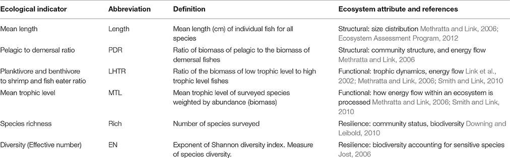
Table 1. Ecological indicators.
Pressure Indicators
A variety of both anthropogenic and environmental variables were selected to reflect pressures on ecosystems (Table 2). Landings (total live weight of commercial species landed weighted by the area of each study ecosystem) and exploitation (the ratio of landings to estimated total biomass of the LME from fishery-independent surveys) served as measures of commercial fishing. We also included a 1-year lag for both landings and exploitation to account for any lagged effects of commercial fishing (Large et al., 2015b). Other variables that track yearly fluctuations in anthropogenic pressures beyond commercial fishing such as, annual human population increase from coastal states that are part of the LME and annual changes in Gross Domestic Product of the coastal community (GDP) demand were also considered (Table 2).
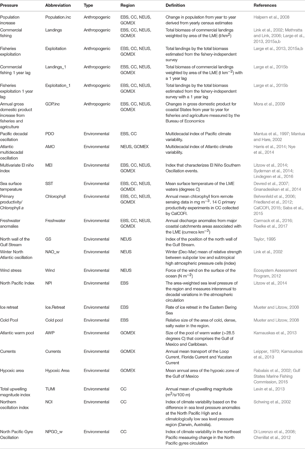
Table 2. Pressure variables from the Alaska (EBS), California Current (CC), Northeast US (NEUS), and Gulf of Mexico (GOMEX) ecosystems.
Environmental variables that influence ecosystem circulation patterns, primary production, availability of nutrients, and vertical mixing were chosen for all LMEs, namely Sea Surface Temperature (SST), and broad scale climatological indicators such as, Pacific Decadal Oscillation (PDO; for the Pacific coast regions), Atlantic Multidecadal Oscillation (AMO; for the Atlantic coast regions), or Multivariate El Niño Index (MEI for all regions). A measure of system production was included (Chlorophyll a). A wide range of other environmental variables that were specific to a given region, for instance ice cover or hypoxic area, were also considered (Table 2).
Statistical Analysis
Gradient Forest Analysis
We used random forest and gradient forest methods on time series of a suite of ecological indicators (Table 1) to assess the importance of anthropogenic and environmental pressures (Table 2) on ecosystems (R package randomForest, R Core Team, 2011; R package gradientForest, R Core Team, 2012) and to identify ecosystem-level thresholds across pressure gradients for each LME. Random forests are methods that can be used to examine multiple responses to pressures. Random forests are comprised of regression tress (or classification trees), where indicators are partitioned into two groups at a specific split value for each pressure to maximize homogeneity within each grouping (Ellis et al., 2012). An independent bootstrap sample of data (resampled with replacement) builds each tree for a given number of simulations. The goodness-of-fit (R2) is partitioned among the pressures and an overall importance is determined by averaging this goodness-of-fit across indicators and time (years). The data not selected in the bootstrap sample (or out-of-bag data) is used to provide cross validations of the generalized error estimates. The synthesized outputs have high classification accuracy and account for interactions among predictor variables.
While random forests are useful for quantifying the ability of pressure variables to predict response variables, gradient forests integrate individual random forest analyses over many response variables and are also used to identify thresholds in those indicator responses along anthropogenic and environmental pressure gradients (Ellis et al., 2012). In gradient forest analysis, the importance values are gathered for each pressure variable for each time period and combined to estimate the threshold of the ecological indicators along the pressure variable. Threshold ranges are determined by calculating the 95% confidence interval about the mean cumulative shift in the aggregate ecological indicator response in R2 units. In short, regression trees indicate the value of potential thresholds and integrating the trees into a “forest” confirms the range of possible shifts and thus delineates thresholds. This range is determined to be where an anticipated ecosystem shift could occur. Detailed description of these methods can be found in Ellis et al. (2012), Baker and Hollowed (2014), and Large et al. (2015a).
Because gradient forest analysis can detect thresholds in a multivariate context, this method is particularly useful for examining thresholds at the ecosystem level (see Pitcher et al., 2011; Baker and Hollowed, 2014; Large et al., 2015b). Consider that a set of species in an ecosystem is sensitive to a particular pressure, but each species within that set responds in a different way. At a given threshold along the pressure gradient, one species is present below that threshold and absent above it; whereas another species exhibits the opposite response at the same threshold. The gradient forest analysis would likely have the first (and most important) split point close to the value of that threshold, thus revealing cumulative importance about the ecosystem threshold (Ellis et al., 2012).
Generalized Additive Models
We used a set of complementary analyses to further examine the multivariate ecosystem trends across pressure variables and to confirm that detected thresholds are robust. We first distilled all of the ecological indicators used in the gradient forest analysis in each LMEinto ecosystem trends using Dynamic Factor Analysis (DFA; R package MARSS, R Core Team, 2013). DFA is a multivariate technique used to identify, detect common patterns in a set of time series (Zuur et al., 2003a,b). We considered two structures for the error covariance matrix R: (1) diagonal and equal and (2) diagonal and unequal (Zuur et al., 2003b; Large et al., 2015a). Diagonal and equal covariance matrices consider the same process variance across all-time series, while diagonal and unequal covariance matrices consider unique variance values for each time series. We selected the ecosystem trends for each region dependent on the DFA model with the lowest AICc score (Hurvich and Tsai, 1989).
Using the best model for the ecosystem, we then used Generalized Additive Models (GAM; R package mgcv, R Core Team, 2014) to examine significant ecosystem trend changes (regions of inflection) as a response to individual pressures (both environmental and anthropogenic) using methods specified in Large et al. (2013). In some instances the DFA model indicated that multiple trends were significant for each LME, in which case, we tested them all in subsequent analyses. We used the GAM models with the formula:
where Y is the ecosystem trend derived from the DFA model, α is held constant, X is the pressure variable, S() is the smoothing function and ε is error. Models that had an estimated p-value > 0.05, estimated degrees of freedom close to the lower limit, and that had generalized cross validation (GCV) scores that decreased when the smoothing term was removed from the models were considered to be linear (Wood, 2004). In this study, GAMs were run with and without a smoothing function to determine the appropriate use of a GAM (with smoothing term) over a GLM (generalized linear model; i.e. GAM without smoothing term). All models had a higher GCV score with the GAM smoother and no GLMs were considered in subsequent analyses. Significant trends and thresholds were determined by examining significant zero crossings of the first and second derivative (as in Large et al., 2013).
A potential strength and weakness of this approach is that it does not rely on a priori identification of functional relationships between response and pressure time-series. The pressure response relationships in this study are multivariate and therefore represent cumulative responses. As such the nature of the ecosystem trend and interpretations of the GAMs will identify threshold points along pressure gradients irrespective of the specific functional responses of each individual ecological indicator to pressure variables. In some cases, the direction of the response of the ecosystem trend against a given pressure may appear to be counterintuitive due to negative factor loadings of the DFA trends (Supplement 1). This combination of analyses, however, offers confirmation (when contrasted with other analyses like gradient forest analysis) of where these threshold ranges are occurring for a total ecosystem response to a given pressure in an LME that allows for comparisons between ecosystems.
Results
Model Performance
The total model prediction performance from the gradient forest analysis (the proportion of variance explained in a random forest) averaged across the suite of ecological indicators from each LME ranged from 0.01 to 0.07 (R2s; Table 3). The model prediction performance for the cumulative ecological indicators had a range of 0–0.30 (R2s), which is consistent with other studies using similar analyses by Large et al. (2015b; 0–0.21 R2s), Pitcher et al. (2011; 0–0.35 R2s), but lower than Baker and Hollowed (2014; 0–0.77 R2s). These model prediction values may appear low; however, in studies with similar results using aggregated ecological indicator data (containing more unexplained variability than raw species abundance metrics) the gradient forest was still able to identify important variables and thresholds (Large et al., 2015b). In contrast to these past studies, this particular analysis focused on cross-ecosystem comparisons and only included ecological indicators that were transferrable across the differing LMEs into the analysis. Inclusion of LME-specific ecological indicators (e.g., longhorn sculpin in the Northeast US; Methratta and Link, 2006) improved the variance explained, but would not allow for true cross-ecosystem comparisons, thus they were excluded from this particular study and account for the lower overall variance explained. Additionally, and more to the point in this comparative study, although the variance explained may be low, multiple (but very different) statistical analyses yielded similar threshold points both within and across ecosystems. In all ecosystems, the ecological indicators that were included in the gradient forest models were mean length (structural) and richness and diversity (resilience) indicators (Table 3). In the Atlantic ecosystems the models maintained a higher number of the ecological indicators in the gradient forest analysis with the fewest in the Alaska ecosystem.
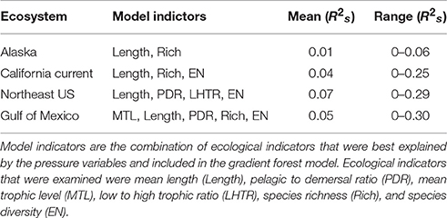
Table 3. Mean Model Performance (R2s) of the out-of-bag samples for the ecological indicators in each region from the gradient forest analyses.
Important Pressure Variables
Both the gradient forest analyses and GAMs did not identify a single driver that was consistently dominant across the four ecosystems, though fisheries landings was an important predictor in models for all systems (Figure 2, Table 4). Generally, anthropogenic variables ranked high in their impact, explaining a larger portion of the changes in the ecosystem trends (at least three of the five most important pressure variables were anthropogenic for all four regions in the gradient forest analysis) than environmental pressures. GAM relationships between ecosystem trends and pressure variables also showed that a larger number of anthropogenic variables significantly impacted ecosystems compared to environmental variables, given the relatively higher values of deviance explained (Table 4). Trends of pressure variable importance were consistent with the historical understanding of each region, with the Northeast US and California Current being strongly impacted by the anthropogenic pressures assessed. The pressures that were specific to a region (e.g., ice cover, hypoxic area; Table 2) were ranked less important than the large scale climatic pressures such as, PDO and AMO in explaining patterns of the cumulative ecological indicators. Exploitation had a high impact in the Atlantic regions.
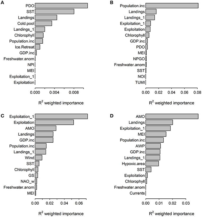
Figure 2. Importance of human and environmental pressure variables across ecological indicator outputs (R2) from the gradient forest analyses for (A) Alaska, (B) California Current, (C) Northeast US, (D) Gulf of Mexico.
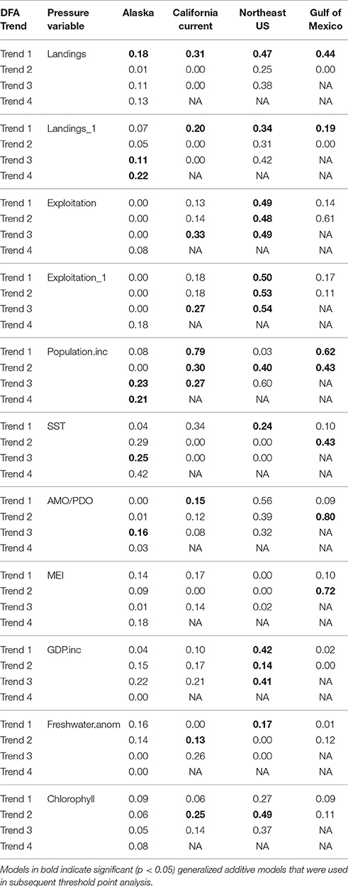
Table 4. Deviance explained for the generalized additive model results for each ecosystem trend (DFA Trend) and pressure variable (using variables common in all ecosystems).
Quantitative Thresholds
Common landings and exploitation thresholds of ~2–4.5 t km−2 landings and ~20–40% exploitation of the total estimated biomass were detected with the gradient forest analyses (Figures 3A,C), bearing in mind that the relative importance of exploitation was low in Alaska and the Gulf of Mexico (Figure 2). Individual thresholds of ecological indicators showed how structural, functional and biodiversity properties of each ecosystem shifted across individual pressure gradients (Figure 4; see Supplement 2). Lagged fishing pressures (landings and exploitation) showed very similar threshold mean and ranges to their non-lagged counterparts (Figures 3B,D). This was also confirmed by the GAM of ecosystem trends (Table 4). The thresholds identified by the GAMs of ecosystem trends along pressure gradients were similar to the thresholds identified by the gradient forest analysis, indicating these ecosystem-level thresholds are robust (Figure 5; see Supplementary Materials). Ecosystem thresholds in response to yearly human population increases were lowest in coastal communities that were (already) most densely populated (Northeast US, Gulf of Mexico); in the lowest populated regions (Alaska) the mean thresholds were highest and they had the widest range (Figure 3E). Yearly changes in the GDP showed ecosystem shifts occurring at higher GDP increases in the Northeast US, Gulf of Mexico, and California Current, compared to Alaska where large ranges of GDP were observed (Figure 3F). SST showed differing thresholds between regions that were unique to the specific ecosystems, largely reflective of the latitudinal position of each ecosystem (Figure 3G). Thresholds for ecological indicators occurred in more positive phases of the AMO, PDO, and MEI (Figures 3H,I), although these tended to have a wide range of threshold. Freshwater anomalies generally ranked lower in terms of importance in explaining ecosystem shifts, but showed a wide threshold region in the California Current (Figure 3J). Chlorophyll a had a higher and wider threshold range in California Current (Figure 3K), indicating that higher levels of primary production in terms of chlorophyll concentration is an important driver there, likely due to upwelling. The three other regions indicate a basal concentration of ~0.7 mg m−3 chlorophyll a to avoid ecosystem shifts (Figure 3K).
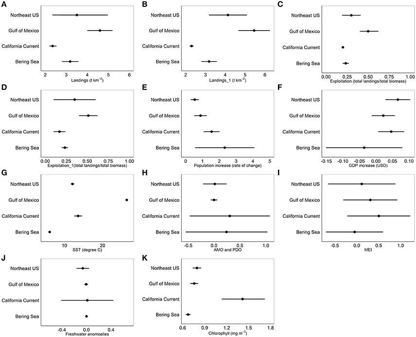
Figure 3. Mean thresholds and 95% CI ranges for (A) Landings, (B) 1 year lagged landings, (C) Exploitation, (D) 1 year lagged exploitation, (E) Population increase of the coastal community, (F) Gross Domestic Product of the coastal community, (G) Sea Surface Temperature, (H) Atlantic Multidecadal Oscillation and Pacific Decadal Oscillation, (I) Multivariate ENSO Index, (J) Freshwater anomalies, and (K) Chlorophyll concentration from the gradient forest analysis for Alaska (Bering Sea), California Current, Northeast US and Gulf of Mexico.
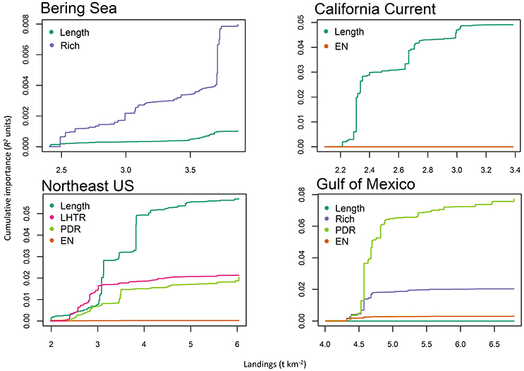
Figure 4. Cumulative shifts (in R2 units) of ecological indicator value in response to landings (t km−2) from the gradient forest analyses for Alaska (Bering Sea), California Current, Northeast US, and Gulf of Mexico. Thresholds are defined as a steep increase in ecological indicator response to a pressure. Ecological indicators are mean length of catch (Length), species richness (Rich), pelagic to demersal ratio (PDR), low to high trophic ratio (LHTR), species diversity (EN).
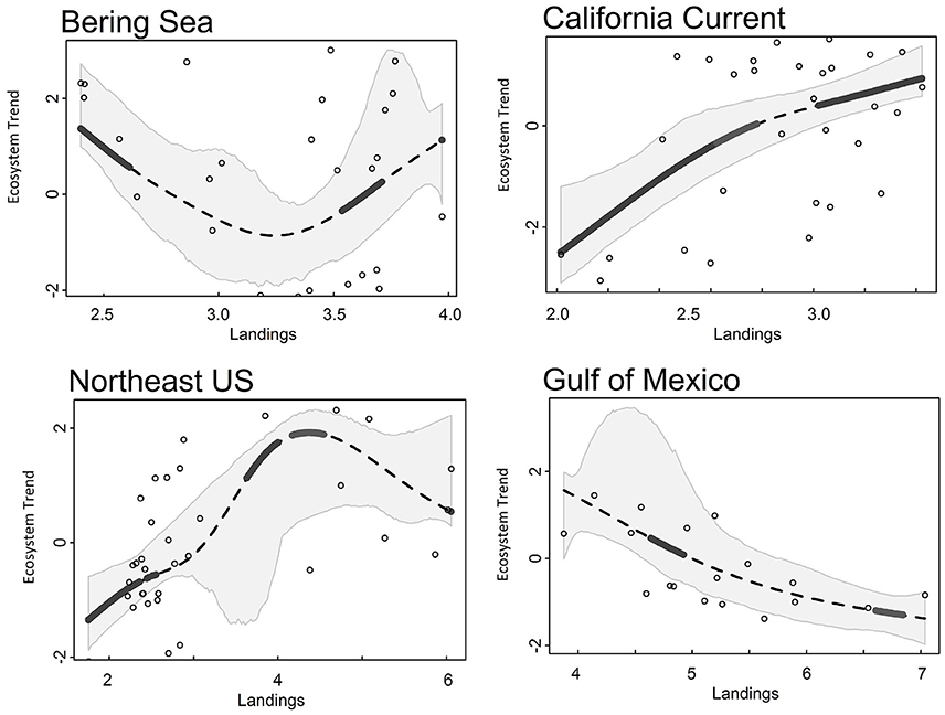
Figure 5. Ecosystem trend (Trend 1 for all LMEs) responses to landings (t km−2) from Alaska (Bering Sea), California Current, Northeast US, and Gulf of Mexico ecosystems. Dotted lines are the smoothed GAM line, gray polygons surrounding the trend line are 95% CI, solid black lines indicate a significant threshold region.
The gradient forest analysis identified the relative size of the cold pool in Alaska as the only region specific pressure variable that ranked within the top five important pressures in explaining ecosystem shifts (Figure 2). The ecosystem thresholds occurred when the cold pool was ~0.2–0.3x relative to the previous year. Ecosystem thresholds along ice retreat index gradients were ~10–50%, while thresholds along north Pacific index were ~−2.0 to 0. In the California Current, ecosystem thresholds were around ~−1.0 to 1.0 for mean annual north Pacific gyre oscillation, 3,000 m3 s−1 100 m−1 total upwelling magnitude index and northern oscillation index at ~−4. Region specific thresholds in the Northeast US were between ~−2.0 and 2.0 for winter north Atlantic oscillation, ~ 0.06–0.07 N m−2 for wind stress and ~1.0–1.3 GS. Ecological indicator thresholds along gradients of mean current transport in the Gulf of Mexico had the lowest importance for the regions according to the gradient forest analysis (Figure 2). Hypoxic area (threshold at ~1.5–2.0 × 10⁴ km2) and Atlantic warm pool (threshold at ~2.0–2.5 × 10⁶ km2) in the Gulf of Mexico explained 0.01 and 0.012 of the ecological indicator response, respectively; which was relatively low compared to other pressure variables in that LME.
Discussion
Patterns in Ecosystem Trends and Thresholds
Our results demonstrate that there are consistent patterns in ecosystem response from common pressures across four large marine ecosystems, and despite multiple potential mechanisms, the detected trends and thresholds to such pressures in these ecosystems were remarkably repeatable. Although each ecosystem examined has different socio-economic histories (Hollowed et al., 2011; Link et al., 2011a; Karnauskas et al., 2013; Levin et al., 2013), different levels of population density, and differential reliance on living marine resources that vary in the use of marine habitats and ultimately shape the stability of the ecosystems, there are a number of common trends that are surprisingly consistent across all ecosystems. These common trends would be difficult to detect if not examined at the ecosystem-level and in a multivariate context, both in terms of detecting baseline reference points and observing emergent properties of marine ecosystems. That these common trends and thresholds exist is insightful for both further understanding of marine ecosystems, as well as management thereof.
One key result is that, at an ecosystem-level, removals of biomass (via landings-based exploitation) do have repeatable and consistent thresholds. There are different ecological mechanisms in which such ecosystem-level responses can be observed, but consistently there is an impact to overall size, congruent with overfishing theory, as well as tendencies toward smaller organisms with hyper-exploitation (Pauly et al., 1998; Pauly and Palomares, 2005; Shackell et al., 2010; Darimont et al., 2015; Worm and Paine, 2016). This exploitation impacts the biomass composition in an entire ecosystem, shifting either biodiversity or measures of biomass ratios (e.g., pelagic to demersal) and implies that exploitation selectively impacts certain facets of an ecosystem consistent with what is known for the ecological effects of targeted fisheries (Shin et al., 2005; Jennings and Collingridge, 2015). Additionally, some form of broad-scale climate forcing is regularly identified as a key driver of ecosystem-level responses. The ecological mechanisms for this can vary, but largely filter through changes in vital rates and related bioenergetics processes (Holsman et al., 2016).
Another commonality was that when examining the impacts of the pressure variables to cumulative ecosystem responses, anthropogenic pressures rank high. Due to the pressure-response relationship of these analyses, this does not necessarily reflect the current status of a given ecosystem, but rather implies that certain pressures have heavily impacted these ecosystems within the history of the time series analyzed. This is not to say that environmental pressures are not important; rather that the anthropogenic pressures tended to more consistently emerge as clearer features that impact observed ecosystem dynamics.
As a particular example of such anthropenic pressures, in all the ecosystems, landings have decreased since the 1970s and 1980s, and some fish stocks have experienced a phase of rebuilding (Rosenberg et al., 2007; Worm et al., 2009; Lotze et al., 2011). Ecosystem responses to commercial fishing are surprisingly consistent in the four regions examined in this study. Ecosystem thresholds were observed at landings of ~2–4.5 t km−2 and fisheries exploitation of ~20–40% of the total estimated biomass. All landings estimates fall within previously determined ecosystem-level surplus production model threshold estimates of 1–6 t km−2 (Bundy et al., 2012; Link et al., 2012; Lucey et al., 2012), further corroborating the robustness of a potentially universal ecosystem-level fisheries yield, at least in the northern hemisphere.
Lower population increases and higher GDP in coastal communities were related to ecosystem shifts where population density is highest (population density of Northeast US: ~300 indv km−2). These threshold values increased with decreasing population densities (Gulf of Mexico: ~56 indv km−2, California Current: ~50 indv km−2. Alaska: ~0.5 indv km−2; U.S. Census Bureau, 2016). Human migration toward more heavily populated areas appears to have a disproportionately large impact on ecosystems. This could relate to a longer history of commercial fishing in a particular region or issues with urban infrastructure (e.g., sewage treatment, erosion prevention). Likely, pressures relating to human population increase act cumulatively to account for these patterns in ecosystem shifts (Halpern et al., 2008; Stallings, 2009; Madin et al., 2016). The Northeast US, California Current, and Gulf of Mexico regions exhibited higher annual GDP increases which were related to ecosystem shifts, compared to Alaska where ecosystem shifts occurred when GDP was both increasing and decreasing. There was a wider range where ecosystem shifts could occur along gradients of population and GDP increase in Alaska, suggesting that less infrastructure, fewer types of industry or lower climate regulation influence ecosystem dynamics and stability (Li and Fang, 2014).
In terms of environmental pressures, another commonality was evidence that all ecosystems appear to influenced by multi-annually varying climate drivers, albeit seen via different indices in each region. The discovery of large-scale climate patterns have been an important step in connecting climate to ecological, biological, and oceanographic patterns in marine ecosystems (Mantua and Hare, 2002; Alheit et al., 2014). Of the environmental drivers examined in this study, the large-scale climate drivers (PDO and AMO) were important in explaining ecosystem shifts when examined at a yearly time scale. Seasonal patterns of climate pressures, however, were not examined in this study to maintain consistency with other indicator and pressure variables, but other relationships and thresholds may certainly exist at different time scales. Both positive PDO and AMO anomalies are associated with dry, hot temperatures in the U.S. (McCabe et al., 2004) and generally correlate positively with SST anomalies that subsequently can cause a shallower ocean mixed layer and lower primary productivity (Mantua and Hare, 2002; Nye et al., 2014). When PDO and AMO anomalies appear to be positive, the ecosystem shifts toward a threshold response. Patterns of chlorophyll across all four ecosystems indicate a base level of primary productivity needed for sustainable fisheries at chlorophyll a concentrations of ~0.7 mg m−3, noting that chlorophyll concentration is positively associated with fisheries yields (Friedland et al., 2012). In the California Current, ecosystem shifts were observed at higher concentrations of chlorophyll which are linked periods of strong upwelling, but ecosystem stability is maintained at lower chlorophyll concentrations (Kahru et al., 2012). Scatterplots of monthly fisheries yields vs. chlorophyll concentration by Friedland et al. (2012) show spikes in observed fisheries yields when chlorophyll concentrations were at or above ~0.7 mg m−3.
The analyses in this study were not used to examine specific mechanistic links between specific pressures and responses, but rather to identify and compare significant threshold ranges of ecosystems (represented by indicators) along pressure gradients. Individual ecological indicator thresholds can also be examined across individual pressure gradients to determine specific reference points at the single indicator level (e.g., Samhouri et al., 2010; Large et al., 2013). This allows for the specific examination of shifts across gradients of individual ecological indicators that can then be examined using other methods (such as, Generalized Linear Models) to determine a trend or directional shift. While doing so would further elucidate the dynamics of a given ecosystem, this study is primarily aimed at examining the location of ecosystem thresholds across pressure gradients across ecosystems. We acknowledge that further insight into individual indicator trends and thresholds are important to gain a fuller understanding of a given ecosystem. We also assert that comparisons across ecosystems, that then detect common trends and thresholds, are equally powerful.
Thresholds as Reference Points in Management
Mechanistic links have been made between fisheries production and multiple drivers including fishing, trophodynamics, and the environment (Gaichas et al., 2012a,b; Holsman et al., 2012; Link et al., 2012; Pranovi et al., 2014; Longo et al., 2015). Multivariate thresholds analyses enable scientists and policy makers to present the complexity of multiple pressures on whole ecosystems in a way that is easier to communicate and comprehend (Peterman, 2004; Large et al., 2015a,b). The methods presented here are complex, in terms of statistical analyses, but are able to offer clear ecosystem-level outputs of threshold ranges across pressure gradients. As such, thresholds provide a powerful tool to delineate and communicate quantifiable tipping points for ecosystems (Foley et al., 2015).
Each ecosystem in this study has, at some stage in the last half century, experienced overfishing (Bakkala et al., 1979; Rosenberg et al., 2007; Walters et al., 2008; Link et al., 2011a; Miller et al., 2014). The impacts of overfishing are complex, but well researched. For example, it has been found that the concentration of fishing on large, predatory species can destabilize ecosystems, resulting in a loss of biodiversity and increasing blooms of lower-trophic organisms, often undesirable species like jellyfish (Pauly et al., 1998; Purcell et al., 2007). More recently, the position of humans within food-webs has been categorized as “hyperkeystone” (Worm and Paine, 2016) or as “super predators” (Milius, 2015), indicating that the current impacts of humans on food webs (marine or otherwise) could lead not only to lower abundances of predatory species, but also size-stunted predator populations with an impaired ability to regulate prey species even in rebuilding scenarios (Darimont et al., 2015). Here we present ecosystem thresholds that can be used as reference points to support coordinated efforts to develop sustainable fisheries via EBM policies that support rebuilding strategies for depleted fish stocks, ecosystem aggregate yield limits, and to explore the social tradeoffs and potential social benefits of changing how we use living marine resources (Murawski, 2000; Balmford, 2002; Howarth and Farber, 2002; Rosenberg et al., 2007; Worm et al., 2009; Khan and Neis, 2010; Link, 2010; Plagányi et al., 2014; DePiper et al., in press).
The thresholds developed here can also be used to build proactive strategies to avoid regime shifts due to overfishing, population increase and climate change, particularly when explored through simulation modeling (Samhouri et al., 2010; Fulton et al., 2011; Fay et al., 2013, 2015; Large et al., 2013). In particular, given the strength of bottom up controls on the systems we evaluated, climate change may be of increasing impact. There have been major breakthroughs in understanding how long-term climatic events and climate change will impact marine species. Many marine communities are predicted to have continued impact by changes in mean SST and are predicted to respond in numerous ways from range shifts (Pinsky and Fogarty, 2012; Gattuso et al., 2015; Heenan et al., 2015) to phenological shifts (Parmesan, 2006; Brown et al., 2016). While the outcomes of climate change are predicted to be overwhelmingly negative, there may be some economic and social benefits for well-managed fisheries in warming scenarios (Barange et al., 2014). Warming climate events in the Gulf of Alaska during the 1970s and 1980s caused dramatic shifts in catch compositions of groundfish, and actually increased the catch biomass of higher trophic-level groundfish by over 250% (Anderson and Piatt, 1999). Anchovy and sardines are known to have multidecadal regime shifts in the Pacific Ocean due to natural, long-term climate variability (Chavez et al., 2003). This can drastically change the catch compositions of these ecosystems over long periods of time and it is important to understand the consequences of unintentionally overfishing during these temporary regime shifts for the long-term sustainability of marine ecosystems. Systems approaches to management, including EBM, can contribute to successful resilience of ecosystems by improving the ability to detect and react to ecological feedbacks (Hughes et al., 2005). Climate thresholds presented in this study can be incorporated into local resource and ocean management and used to develop rules around total harvests of specific species based on known or predicted distributional shifts (Link et al., 2011b; Pinsky et al., 2013; Heenan et al., 2015).
While the location of ranges of ecosystem-level thresholds along both human and environmental pressure gradients are easily interpreted, these insights are best made against a backdrop of dynamic biological and environmental conditions. While it is easy for many to agree that benefits to human well-being correlate positively with ecosystem services, it is often difficult to incorporate these ideas into management (Arkema et al., 2015). Social indicators that examine the mechanistic links between human well-being and ecosystems are being examined, but are generally underdeveloped (McShane et al., 2011; Colburn and Jepson, 2012; Howe et al., 2014; Pollnac et al., 2015; Yang et al., 2015). Studies such as the one undertaken here address issues from an ecosystem-based fisheries management standpoint, but the inclusion of more social indicators (such as, GDP and human population increases) would move this work more fully toward EBM. Improving and expanding on indicators for human well-being would greatly enhance the ability to examine thresholds for societal needs within the context of this study, but also to examine the inherent tradeoffs between the needs of people and marine ecological sustainability and conservation (Dearing et al., 2014; DePiper et al., in press).
Conclusion
There is a sense of urgency to develop management and policy that supports ecosystem-level sustainability and conservation given the current global demand for living marine resources and marine ecosystem services (Pauly and Palomares, 2005; Mollmann et al., 2014; Worm and Paine, 2016). The thresholds presented in this study offer guidance toward developing quantifiable, defensible and robust reference points in policy and management for sustainable marine ecosystems. With the variety of ecosystem types examined (sub-polar, upwelling, temperate, and sub-tropical), these thresholds could become operational not only in the US, but also in other comparable systems globally. They are particularly useful as a baseline to develop similar reference points and policy guidelines in regions that lack sufficient data to develop analogously derived quantitative thresholds. Using ecosystem-level thresholds to make cross-ecosystem comparisons reveal interesting emergent properties that unify the current understanding of large-scale climate drivers, human population growth and commercial fishing which will further enhance global progress toward EBM.
Author Contributions
JT authored/drafted, analyzed, provided final approval, and is accountable for this manuscript. JL and SL provided intellectual content, revised, provided final approval, and is accountable for this manuscript. RS provided intellectual content, revisions, final approval and is accountable for this manuscript. KA, KF, JG, EH, KH, MK, NT, SZ and JS provided data, revisions, final approval, and are accountable for this manuscript.
Conflict of Interest Statement
The authors declare that the research was conducted in the absence of any commercial or financial relationships that could be construed as a potential conflict of interest.
Acknowledgments
We thank the research vessel crews and scientific staff at NOAA-Fisheries, whose hard work make such studies possible. We thank S. Benjamin at the NEFSC (Social Sciences Branch) for map creation. We also thank S. Lucey (NEFSC) and I. Kaplan (NWFSC) for assisting in data procurement and helpful comments. We also thank internal reviewers S. Gaichas, K. Craig, and K. Osgood for their helpful comments and suggestions. This work was supported by a NOAA Postdoctoral Fellowship to JT and funding from the IEA Program. The findings and conclusions in the paper are those of the authors and do not necessarily represent the views of the National Marine Fisheries Service, NOAA. Reference to trade names does not imply endorsement by the National Marine Fisheries Service, NOAA.
Supplementary Material
The Supplementary Material for this article can be found online at: https://www.frontiersin.org/article/10.3389/fmars.2017.00282/full#supplementary-material
References
Alheit, J., Drinkwater, K. F., and Nye, J. A. (2014). Introduction to special issue: Atlantic multidecadal oscillation-mechanism and impact on marine ecosystems. J. Mar. Syst. 133, 1–3. doi: 10.1016/j.jmarsys.2013.11.012
Anderson, P. J., and Piatt, J. F. (1999). Community reorganization in the Gulf of Alaska following ocean climate regime shift. Mar. Ecol. Prog. Ser. 189, 117–123. doi: 10.3354/meps189117
Arkema, K. K., Verutes, G. M., Wood, S. A., Clarke-Samuels, C., Rosado, S., Canto, M., et al. (2015). Embedding ecosystem services in coastal planning leads to better outcomes for people and nature. Proc. Natl. Acad. Sci. U.S.A. 112, 7390–7395. doi: 10.1073/pnas.1406483112
Baker, M. R., and Hollowed, A. B. (2014). Delineating ecological regions in marine systems: Integrating physical structure and community composition to inform spatial management in the eastern Bering Sea. Deep Sea Res. Part II Top. Stud. Oceanogr. 109, 215–240. doi: 10.1016/j.dsr2.2014.03.001
Bakkala, R., Hirschberger, W., and King, K. (1979). The groundfish resources of the Eastern Bering Sea and Aleutian-Islands regions. Mar. Fish. Rev. 41, 1–24.
Balmford, A. (2002). Economic reasons for conserving wild nature. Science 297, 950–953. doi: 10.1126/science.1073947
Barange, M., Merino, G., Blanchard, J. L., Scholtens, J., Harle, J., Allison, E. H., et al. (2014). Impacts of climate change on marine ecosystem production in societies dependent on fisheries. Nat. Clim. Change 4, 211–216. doi: 10.1038/nclimate2119
Behrenfeld, M. J., O'Malley, R. T., Siegel, D. A., McClain, C. R., Sarmiento, J. L., Feldman, G. C., et al. (2006). Climate-driven trends in contemporary ocean productivity. Nature 444, 752–755. doi: 10.1038/nature05317
Bigagli, E. (2015). The EU legal framework for the management of marine complex social–ecological systems. Mar. Policy 54, 44–51. doi: 10.1016/j.marpol.2014.11.025
Brown, C. J., O'Connor, M. I., Poloczanska, E. S., Schoeman, D. S., Buckley, L. B., Burrows, M. T., et al. (2016). Ecological and methodological drivers of species' distribution and phenology responses to climate change. Glob. Change Biol. 22, 1548–1560. doi: 10.1111/gcb.13184
Bundy, A., Bohaboy, E. C., Hjermann, D. O., Mueter, F. J., Fu, C., and Link, J. S. (2012). Common patterns, common drivers: comparative analysis of aggregate surplus production across ecosystems. Mar. Ecol. Prog. Ser. 459, 203–218. doi: 10.3354/meps09787
Bundy, A., Shannon, L., Rochet, J., and Neira, S. (2010). The Good ( ish ), the bad and the ugly : a tripartite classification of ecosystem trends. ICES J. Mar. Sci. 67, 745–768. doi: 10.1093/icesjms/fsp283.
CalCOFI (2015). California Cooperative Oceanic Fisheries Investigations Data. Available at: http://calcofi.org/data.html (Accessed August 1, 2015).
Carmack, E. C., Yamamoto-Kawai, M., Haine, T. W. N., Bacon, S., Bluhm, B. A., Lique, C., et al. (2016). Freshwater and its role in the Arctic marine system: sources, disposition, storage, export, and physical and biogeochemical consequences in the Arctic and global oceans. J. Geophys. Res. G Biogeosci. 121, 675–717. doi: 10.1002/2015JG003140
Chavez, F. P., Ryan, J., Lluch-Cota, S. E., and Niquen, C., M. (2003). From anchovies to sardines and back: multidecadal change in the pacific ocean. Science 299, 217–221. doi: 10.1126/science.1075880
Chenillat, F., Riviére, P., Capet, X., Di Lorenzo, E., and Blanke, B. (2012). North Pacific gyre oscillation modulates seasonal timing and ecosystem functioning in the California Current upwelling system. Geophys. Res. Lett. 39, 1–6. doi: 10.1029/2012GL053111
Colburn, L. L., and Jepson, M. (2012). Social indicators of gentrification pressure in fishing communities: a context for social impact assessment. Coast. Manage. 40, 289–300. doi: 10.1080/08920753.2012.677635
Coll, M., and Lotze, H. K. (2016). “Ecological indicators and food-web models as tools to study historical changes in marine ecosystems,” in Perspectives on Oceans Past, eds K. Schwerdtner Máñez and B. Poulsen (Dordrecht: Springer Netherlands), 103–132.
Coll, M., Libralato, S., Tudela, S., Palomera, I., and Pranovi, F. (2008). Ecosystem overfishing in the ocean. PLoS ONE 3:e3881. doi: 10.1371/journal.pone.0003881
Conner, J., and Lauth, R. R. (2017). Results of the 2016 Eastern Bering Sea Continental Shelf Bottom Trawl Survey of Groundfish and Invertebrate Resources. U.S. Dep. Commer., NOAA Tech. Memo. NMFS-AFSC-352, C-159.
Connell, S. D., Fernandes, M., Burnell, O. W., Doubleday, Z. A., Griffin, K. J., Irving, A. D., et al. (in press), Testing for thresholds of ecosystem collapse in seagrass meadows. Conserv. Biol. doi: 10.1111/cobi.12951
Constable, A. J. (2011). Lessons from CCAMLR on the implementation of the ecosystem approach to managing fisheries. Fish Fish. 12, 138–151. doi: 10.1111/j.1467-2979.2011.00410.x
Constable, A. J., de la Mare, W. K., Agnew, D. J., Everson, I., and Miller, D. (2000). Managing fisheries to conserve the Antarctic marine ecosystem: practical implementation of the Convention on the Conservation of Antarctic Marine Living Resources (CCAMLR). ICES J. Mar. Sci. 57, 778–791. doi: 10.1006/jmsc.2000.0725
Crain, C. M., Kroeker, K., and Halpern, B. S. (2008). Interactive and cumulative effects of multiple human stressors in marine systems. Ecol. Lett. 11, 1304–1315. doi: 10.1111/j.1461-0248.2008.01253.x
Darimont, C. T., Fox, C. H., Bryan, H. M., and Reimchen, T. E. (2015). The unique ecology of human predators. Science 349, 858–860. doi: 10.1126/science.aac4249
Dearing, J. A., Wang, R., Zhang, K., Dyke, J. G., Haberl, H., Hossain, M. S., et al. (2014). Safe and just operating spaces for regional social-ecological systems. Glob. Environ. Change 28, 227–238. doi: 10.1016/j.gloenvcha.2014.06.012
DePiper, G. S., Gaichas, S. K., Lucey, S. M., Pinto, P., Anderson, M. R., Breeze, H., et al. (in press). Operationalizing integrated ecosystem assessments within a multidisciplinary team: lessons learned from a worked example. ICES J. Mar. Sci. doi: 10.1093/icesjms/fsx038
Devred, E., Sathyendranath, S., and Platt, T. (2007). Delineation of ecological provinces using ocean colour radiometry. Mar. Ecol. Prog. Ser. 346, 1–13. doi: 10.3354/meps07149
Di Lorenzo, E., Schneider, N., Cobb, K. M., Franks, P. J. S., Chhak, K., Miller, A. J., et al. (2008). North Pacific Gyre Oscillation links ocean climate and ecosystem change. Geophys. Res. Lett. 35, 2–7. doi: 10.1029/2007GL032838
Doney, S. C. (2010). The growing human footprint on coastal and open-ocean biogeochemistry. Science 328, 1512–1516. doi: 10.1126/science.1185198
Downing, A. L., and Leibold, M. A. (2010). Species richness facilitates ecosystem resilience in aquatic food webs. Freshw. Biol. 55, 2123–2137. doi: 10.1111/j.1365-2427.2010.02472.x
Ecosystem Assessment Program (2012). Ecosystem Status Report for the Northeast Shelf Large Marine Ecosystem - 2011. Woods Hole, MA, USA.
Ellis, N., Smith, S. J., and Pitcher, C. R. (2012). Gradient forests: calculating importance gradients on physical predictors. Ecology 93, 156–168. doi: 10.1890/11-0252.1
Fay, G., Large, S. I., Link, J. S., and Gamble, R. J. (2013). Testing systemic fishing responses with ecosystem indicators. Ecol. Modell. 265, 45–55. doi: 10.1016/j.ecolmodel.2013.05.016
Fay, G., Link, J. S., Large, S. I., and Gamble, R. J. (2015). Management performance of ecological indicators in the Georges Bank finfish fishery. ICES J. Mar. Sci. 72, 1285–1296. doi: 10.1093/icesjms/fsu214
Foley, M. M., Martone, R. G., Fox, M. D., Kappel, C. V., Mease, L. A., Erickson, A. L., et al. (2015). Using ecological thresholds to inform resource management: current options and future possibilities. Front. Mar. Sci. 2:95. doi: 10.3389/fmars.2015.00095
Friedland, K. D., Stock, C., Drinkwater, K. F., Link, J. S., Leaf, R. T., Shank, B. V., et al. (2012). Pathways between primary production and fisheries yields of large marine ecosystems. PLoS ONE 7:e28945. doi: 10.1371/journal.pone.0028945
Fulton, E. A., Link, J. S., Kaplan, I. C., Savina-Rolland, M., Johnson, P., Ainsworth, C., et al. (2011). Lessons in modelling and management of marine ecosystems: the Atlantis experience. Fish Fish. 12, 171–188. doi: 10.1111/j.1467-2979.2011.00412.x
Gaichas, S., Bundy, A., Miller, T., Moksness, E., and Stergiou, K. (2012a). What drives marine fisheries production? Mar. Ecol. Prog. Ser. 459, 159–163. doi: 10.3354/meps09841
Gaichas, S., Gamble, R., Fogarty, M., Benoit, H., Essington, T., Fu, C. H., et al. (2012b). Assembly rules for aggregate-species production models: simulations in support of management strategy evaluation. Mar. Ecol. Prog. Ser. 459, 275–292. doi: 10.3354/meps09650
Garrison, L. (2000). Fishing effects on spatial distribution and trophic guild structure of the fish community in the Georges Bank region. ICES J. Mar. Sci. 57, 723–730. doi: 10.1006/jmsc.2000.0713
Gattuso, J.-P., Magnan, A., Billé, R., Cheung, W. W. L., Howes, E. L., Joos, F., et al. (2015). Contrasting futures for ocean and society from different anthropogenic CO2 emissions scenarios. Science 349:aac4722. doi: 10.1126/science.aac4722
Gnanadesikan, A., Dunne, J. P., and Msadek, R. (2014). Connecting Atlantic temperature variability and biological cycling in two earth system models. J. Mar. Syst. 133, 39–54. doi: 10.1016/j.jmarsys.2013.10.003
Gulf States Marine Fishing Commission, Atlantic States Marine Fisheries Commission, and Puerto Rico Sea Grant College, Program (2015). Annual Report of the Southeast Area Monitoring and Assessment Program (SEAMAP).
Halpern, B. S., Longo, C., Hardy, D., McLeod, K. L., Samhouri, J. F., Katona, S. K., et al. (2012). An index to assess the health and benefits of the global ocean. Nature 488, 615–620. doi: 10.1038/nature11397
Halpern, B. S., Walbridge, S., Slkoe, K. A., Kappel, C. V., Micheli, F., D'Agrosa, C., et al. (2008). A global map of human impact on marine ecosystems. Science 319, 948–952. doi: 10.1126/science.114934
Harris, V., Edwards, M., and Olhede, S. C. (2014). Multidecadal Atlantic climate variability and its impact on marine pelagic communities. J. Mar. Syst. 133, 55–69. doi: 10.1016/j.jmarsys.2013.07.001
Heenan, A., Pomeroy, R., Bell, J., Munday, P. L., Cheung, W., Logan, C., et al. (2015). A climate-informed, ecosystem approach to fisheries management. Mar. Policy 57, 182–192. doi: 10.1016/j.marpol.2015.03.018
Heymans, J. J., Coll, M., Libralato, S., Morissette, L., and Christensen, V. (2014). Global patterns in ecological indicators of marine food webs: a modelling approach. PLoS ONE 9:e95845. doi: 10.1371/journal.pone.0095845
Hollowed, A. B., Aydin, K. Y., Essington, T. E., Ianelli, J. N., Megrey, B. A., Punt, A. E., et al. (2011). Experience with quantitative ecosystem assessment tools in the northeast Pacific. Fish Fish. 12, 189–208. doi: 10.1111/j.1467-2979.2011.00413.x
Holsman, K. K., Essington, T., Miller, T. J., Koen-Alonso, M., and Stockhausen, W. J. (2012). Comparative analysis of cod and herring production dynamics across 13 northern hemisphere marine ecosystems. Mar. Ecol. Prog. Ser. 459, 231–246. doi: 10.3354/meps09765
Holsman, K. K., Ianelli, J., Aydin, K., Punt, A. E., and Moffitt, E. A. (2016). A comparison of fisheries biological reference points estimated from temperature-specific multi-species and single-species climate-enhanced stock assessment models. Deep. Res. Part II Top. Stud. Oceanogr. 134, 360–378. doi: 10.1016/j.dsr2.2015.08.001
Howarth, R. B., and Farber, S. (2002). Accounting for the value of ecosystem services. Ecol. Econ. 41, 421–429. doi: 10.1016/S0921-8009(02)00091-5
Howe, C., Suich, H., Vira, B., and Mace, G. M. (2014). Creating win-wins from trade-offs? Ecosystem services for human well-being: A meta-analysis of ecosystem service trade-offs and synergies in the real world. Glob. Environ. Change 28, 263–275. doi: 10.1016/j.gloenvcha.2014.07.005
Hughes, T. P., Bellwood, D. R., Folke, C., Steneck, R. S., and Wilson, J. (2005). New paradigms for supporting the resilience of marine ecosystems. Trends Ecol. Evol. 20, 380–386. doi: 10.1016/j.tree.2005.03.022
Hurvich, C. M., and Tsai, C.-L. (1989). Regression and time series model selection in small samples. Biometrika 76, 297–307. doi: 10.1093/biomet/76.2.297
Jackson, J. B. C., Kirby, M. X., Berger, W. H., Bjorndal, K. A., Botsford, L. W., Bourque, B. J., et al. (2001). Historical overfishing and the recent collapse of coastal ecosystems. Science 293, 629–639. doi: 10.1126/science.1059199
Jennings, S. (2005). Indicators to support an ecosystem approach to fisheries. Fish Fish. 6, 212–232. doi: 10.1111/j.1467-2979.2005.00189.x
Jennings, S., and Collingridge, K. (2015). Predicting consumer biomass, size-structure, production, catch potential, responses to fishing and associated uncertainties in the world's marine ecosystems. PLoS ONE 10:e0133794. doi: 10.1371/journal.pone.0133794
Kahru, M., Kudela, R. M., Manzano-Sarabia, M., and Greg Mitchell, B. (2012). Trends in the surface chlorophyll of the California Current: merging data from multiple ocean color satellites. Deep. Res. Part II Top. Stud. Oceanogr. 77–80, 89–98. doi: 10.1016/j.dsr2.2012.04.007
Karnauskas, M., Schirripa, M. J., Kelble, C. R., Cook, G. S., and Craig, J. K. (2013). Ecosystem Report for the Gulf of Mexico. NOAA Technical Memorandum NMFS-SEFSC-653, 52.
Kelble, C. R., Loomis, D. K., Lovelace, S., Nuttle, W. K., Ortner, P. B., Fletcher, P., et al. (2013). The EBM-DPSER conceptual model: integrating ecosystem services into the DPSIR framework. PLoS ONE 8:e70766. doi: 10.1371/journal.pone.0070766
Khan, A. S., and Neis, B. (2010). The rebuilding imperative in fisheries: clumsy solutions for a wicked problem? Prog. Oceanogr. 87, 347–356. doi: 10.1016/j.pocean.2010.09.012
Large, S. I., Fay, G., Friedland, K. D., and Link, J. S. (2013). Defining trends and thresholds in responses of ecological indicators to fishing and environmental pressures. ICES J. Mar. Sci. 70, 755–767. doi: 10.1093/icesjms/fst067
Large, S. I., Fay, G., Friedland, K. D., and Link, J. S. (2015a). Critical points in ecosystem responses to fishing and environmental pressures. Mar. Ecol. Prog. Ser. 521, 1–17. doi: 10.3354/meps11165
Large, S. I., Fay, G., Friedland, K. D., and Link, J. S. (2015b). Quantifying patterns of change in marine ecosystem response to multiple pressures. PLoS ONE 10:e0119922. doi: 10.1371/journal.pone.0119922
Leipper, D. F. (1970). A sequence of current patterns in the Gulf of Mexico. J. Geophys. Res. 75, 637–657. doi: 10.1029/JC075i003p00637
Leslie, H. M., and McLeod, K. L. (2007). Confronting the challenges of implementing marine ecosystem-based management. Front. Ecol. Environ. 5, 540–548. doi: 10.1890/060093
Levin, P. S., and Schwing, F. B. (eds.) (2011). Technical Background for an Integrated Ecosystem Assessment of the California Current: Groundfish, Salmon, Green Sturgeon, and Ecosystem Health. U.S. Dept. Commer; NOAA Tech. Memo; NMFS-NWFSC-109, 330.
Levin, P. S., Fogarty, M. J., Murawski, S. A., and Fluharty, D. (2009). Integrated ecosystem assessments: developing the scientific basis for ecosystem-based management of the ocean. PLoS Biol. 7:e14. doi: 10.1371/journal.pbio.1000014
Levin, P. S., Kelble, C. R., Shuford, R. L., Ainsworth, C., Dunsmore, R., Fogarty, M. J., et al. (2014). Guidance for implementation of integrated ecosystem assessments: a US perspective. ICES 71, 1198–1204. doi: 10.1093/icesjms/fst112
Levin, P. S., Wells, B. K., and Sheer, M. B., (eds). (2013). Integrated Ecosystem Assessment of the California Current: Phase II Report. Seattle, WA. Available online at: http://www.noaa.gov/iea/CCIEA-Report/index
Li, G., and Fang, C. (2014). Global mapping and estimation of ecosystem services values and gross domestic product: a spatially explicit integration of national “green GDP” accounting. Ecol. Indic. 46, 293–314. doi: 10.1016/j.ecolind.2014.05.020
Liboiron, M. (2015). Redefining pollution and action: the matter of plastics. J. Mater. Cult. 21, 87–110. doi: 10.1177/1359183515622966
Lindegren, M., Checkley, D. M. Jr., Ohman, M. D., Koslow, J. A., and Goericke, R. (2016). Resilience and stability of a pelagic marine ecosystem. Proc. R Soc. B 283:20151931. doi: 10.1098/rspb.2015.1931
Link, J. S. (2010). Ecosystem-Based Fisheries Management: Confronting Tradeoffs, 1st Edn. New York, NY: Cambridge University Press.
Link, J. S., Brodziak, J. K. T., Dow, D. D., Edwards, S. F., Fabrizio, M. C., Fogarty, M. J., et al. (2002). Status of the Northeast U.S. Continental Shelf Ecosystem. Northeast Fisheries Science Center Reference Document 02–11, Woods Hole, MA.
Link, J. S., Bundy, A., Overholtz, W. J., Shackell, N., Manderson, J., Duplisea, D., et al. (2011a). Ecosystem-based fisheries management in the Northwest Atlantic. Fish Fish. 12, 152–170. doi: 10.1111/j.1467-2979.2011.00411.x
Link, J. S., Gaichas, S., Miller, T. J., Essington, T., Bundy, A., Boldt, J., et al. (2012). Synthesizing lessons learned from comparing fisheries production in 13 northern hemisphere ecosystems: emergent fundamental features. Mar. Ecol. Prog. Ser. 459, 293–302. doi: 10.3354/meps09829
Link, J. S., Nye, J. A., and Hare, J. A. (2011b). Guidelines for incorporating fish distribution shifts into a fisheries management context. Fish Fish. 12, 461–469. doi: 10.1111/j.1467-2979.2010.00398.x
Link, J. S., Pranovi, F., Libralato, S., Coll, M., Christensen, V., Solidoro, C., et al. (2015). Emergent properties delineate marine ecosystem perturbation and recovery. Trends Ecol. Evol. 30, 649–661. doi: 10.1016/j.tree.2015.08.011
Litzow, M. A., Mueter, F. J., and Hobday, A. J. (2014). Reassessing regime shifts in the North Pacific: incremental climate change and commercial fishing are necessary for explaining decadal-scale biological variability. Glob. Change Biol. 20, 38–50. doi: 10.1111/gcb.12373
Longo, C., Hornborg, S., Bartolino, V., Tomczak, M., Ciannelli, L., Libralato, S., et al. (2015). Role of trophic models and indicators in current marine fisheries management. Mar. Ecol. Prog. Ser. 538, 257–272. doi: 10.3354/meps11502
Lotze, H. K., Coll, M., Magera, A. M., Ward-Paige, C., and Airoldi, L. (2011). Recovery of marine animal populations and ecosystems. Trends Ecol. Evol. 26, 595–605. doi: 10.1016/j.tree.2011.07.008
Lucey, S. M., Cook, A. M., Boldt, J. L., Link, J. S., Essington, T. E., and Miller, T. J. (2012). Comparative analyses of surplus production dynamics of functional feeding groups across 12 northern hemisphere marine ecosystems. Mar. Ecol. Prog. Ser. 459, 219–229. doi: 10.3354/meps09825
Madin, E. M. P., Dill, L. M., Ridlon, A. D., Heithaus, M. R., and Warner, R. R. (2016). Human activities change marine ecosystems by altering predation risk. Glob. Change Biol. 22, 44–60. doi: 10.1111/gcb.13083
Mantua, N. J., and Hare, S. R. (2002). The pacific decadal oscillation. J. Oceanogr. 44, 35–44. doi: 10.1023/A:1015820616384
Mantua, N. J., Hare, S. R., Zhang, Y., Wallace, J. M., and Francis, R. C. (1997). A pacific interdecadal climate oscillation with impacts on salmon production. Bull. Am. Meteorol. Soc. 78, 1069–1079. doi: 10.1175/1520-0477(1997)078<;1069:APICOW>2.0.CO;2
McCabe, G. J., Palecki, M. A., and Betancourt, J. L. (2004). Pacific and Atlantic Ocean influences on multidecadal drought frequency in the United States. Proc. Natl. Acad. Sci. U.S.A. 101, 4136–4141. doi: 10.1073/pnas.0306738101
McShane, T. O., Hirsch, P. D., Trung, T. C., Songorwa, A. N., Kinzig, A., Monteferri, B., et al. (2011). Hard choices: Making trade-offs between biodiversity conservation and human well-being. Biol. Conserv. 144, 966–972. doi: 10.1016/j.biocon.2010.04.038
Methratta, E. T., and Link, J. S. (2006). Evaluation of quantitative indicators for marine fish communities. Ecol. Indic. 6, 575–588. doi: 10.1016/j.ecolind.2005.08.022
Milius, S. (2015), Life & evolution: seeing humans as superpredators: many hunting, fishing habits may be unsustainable for prey. Sci. News 188:9. doi: 10.1002/scin.2015.188006008
Miller, R. R., Field, J. C., Santora, J. A., Schroeder, I. D., Huff, D. D., Key, M., et al. (2014). A spatially distinct history of the development of California groundfish fisheries. PLoS One 9:e99758. doi: 10.1371/journal.pone.0099758
Mollmann, C., Folke, C., Edwards, M., and Conversi, A. (2014). Marine regime shifts around the globe : theory, drivers and impacts. Philos. Trans. R. Soc. B 370:20130260. doi: 10.1098/rstb.2013.0260
Mora, C., Myers, R. A., Coll, M., Libralato, S., Pitcher, T. J., Sumaila, R. U., et al. (2009). Management effectiveness of the world's marine fisheries. PLoS Biol. 7:e1000131. doi: 10.1371/journal.pbio.1000131
Mueter, F., and Litzow, M. (2008). Sea ice retreat alters the biogeography of the Bering sea continental shelf. Ecol. Appl. 18, 309–320. doi: 10.1890/07-0564.1
Murawski, S. A. (2000). Definitions of overfishing from an ecosystem perspective. ICES J. Mar. Sci. 57, 649–658. doi: 10.1006/jmsc.2000.0738
Murawski, S. A., Steele, J. H., Taylor, P., Fogarty, M. J., Sissenwine, M. P., Ford, M., et al. (2010). Why compare marine ecosystems? ICES J. Mar. Sci. 67, 1–9. doi: 10.1093/icesjms/fsp221
Nichols, S. (2004). Derivation of Red Snapper Times Series from SEAMAP and Groundfish Trawl Surveys. SEDAR7-DW-1. North Charleston, SC: SEDAR. 28.
Nye, J. A., Baker, M. R., Bell, R., Kenny, A., Kilbourne, K. H., Friedland, K. D., et al. (2014). Ecosystem effects of the Atlantic multidecadal oscillation. J. Mar. Syst. 133, 103–116. doi: 10.1016/j.jmarsys.2013.02.006
Österblom, H., Crona, B. I., Folke, C., and Nyström, M. (2016). Marine ecosystem science on an intertwined planet. Ecosystems 20, 54–61. doi: 10.1007/s10021-016-9998-6
Palialexis, A., Tornero, V., Barbone, E., Gonzalez, D., Hanke, G., Cardoso, A. C., et al. (2014). In-depth Assessment of the EU Member States' Submissions for the Marine Strategy Framework Directive under Articles 8, 9 and 10. JRC Scientific and Technical Reports. Joint Research Centre, Institute for Environment and Sustainability, Ispra.
Parmesan, C. (2006). Ecological and evolutionary responses to recent climate change. Annu. Rev. Ecol. Evol. Syst. 37, 637–669. doi: 10.1146/annurev.ecolsys.37.091305.110100
Pauly, D., and Palomares, M. (2005). Fishing down marine food web: It is far more pervasive than we thought. Bull. Mar. Sci. 76, 197–211.
Pauly, D., Christensen, V., Dalsgaard, J., Froese, R., and Torres, F. Jr., (1998). Fishing down marine food webs. Science (80-. ). 279, 860–863. doi: 10.1126/science.279.5352.860
Peterman, R. M. (2004). Possible solutions to some challenges facing fisheries scientists and managers. ICES J. Mar. Sci. 61, 1331–1343. doi: 10.1016/j.icesjms.2004.08.017
Pinsky, M. L., and Fogarty, M. (2012). Lagged social-ecological responses to climate and range shifts in fisheries. Clim. Change 115, 883–891. doi: 10.1007/s10584-012-0599-x
Pinsky, M. L., Worm, B., Fogarty, M. J., Sarmiento, J. L., and Levin, S. A. (2013). Marine taxa track local climate velocities. Science 341, 1239–1242. doi: 10.1126/science.1239352
Pitcher, C. R., Ellis, N., and Smith, S. J. (2011). Example Analysis of Biodiversity Survey Data with R Package Gradientforest. Gradient Forest Basics.
Plagányi, É. E., Punt, A. E., Hillary, R., Morello, E. B., Thébaud, O., Hutton, T., et al. (2014). Multispecies fisheries management and conservation: tactical applications using models of intermediate complexity. Fish Fish. 15, 1–22. doi: 10.1111/j.1467-2979.2012.00488.x
Politis, P. J., Galbraith, J. K., Kostovick, P., and Brown, R. W. (2014). Northeast Fisheries Science Center Bottom Trawl Survey Protocols for the NOAA Ship Henry B. Bigelow. US Dept Commer; Northeast Fish Sci Cent Ref Doc. 14-06, 138.
Pollack, A. G., Hanisko, D. S., and Ingram, G. W. (2016). Wenchman Abundance Indices from SEAMAP Groundfish Surveys in the Northern Gulf of Mexico. SEDAR49-DW-19. North Charleston, SC: SEDAR. 27.
Pollnac, R. B., Seara, T., and Colburn, L. L. (2015). Aspects of fishery management, job satisfaction, and well-being among commercial fishermen in the northeast region of the United States. Soc. Nat. Resour. 28, 75–92. doi: 10.1080/08941920.2014.933924
Pranovi, F., Libralato, S., Zucchetta, M., and Link, J. S. (2014). Biomass accumulation across trophic levels: analysis of landings for the Mediterranean Sea. Mar. Ecol. Prog. Ser. 512, 201–216. doi: 10.3354/meps10881
Purcell, J. E., Uye, S., and Lo, W. (2007). Anthropogenic causes of jellyfish blooms and their direct consequences for humans: a review. Mar. Ecol. Prog. Ser. 350, 153–174. doi: 10.3354/meps07093
R Core Team (2011). R: A Language and Environment for Statistical Computing. Vienna: R Foundation for Statistical Computing. Available online at: https://www.R-project.org/
R Core Team (2012). R: A Language and Environment for Statistical Computing. Vienna: R Foundation for Statistical Computing. Available online at: https://www.R-project.org/
R Core Team (2013). R: A Language and Environment for Statistical Computing. Vienna: R Foundation for Statistical Computing. Available online at: https://www.R-project.org/
R Core Team (2014). R: A Language and Environment for Statistical Computing. Vienna: R Foundation for Statistical Computing. Available online at: https://www.R-project.org/
R Core Team (2015). R: A Language and Environment for Statistical Computing. Vienna: R Foundation for Statistical Computing. Available online at: https://www.R-project.org/
Rabalais, N. N., Turner, R. E., and Wiseman, W. J. Jr. (2002). Gulf of Mexico Hypoxia, a.k.a. “The Dead Zone.” Annu. Rev. Ecol. Syst. 33, 235–263. doi: 10.1146/annurev.ecolsys.33.010802.150513
Reid, R. N., Almeida, F. P., and Zetlin, C. A. (1999). Essential Fish Habitat Source Document: Fishery Independent Surveys, Data Sources, and Methods. U.S. Dep. Commer. NOAA Tech. Memo. NMFS-NE-122: E-139.
Rice, J. C., and Rochet, M. (2005). A framework for selecting a suite of indicators for fisheries management. ICES J. Mar. Sci. 62, 516–527. doi: 10.1016/j.icesjms.2005.01.003
Roelke, D. L., Li, H.-P., Miller-DeBoer, C. J., Gable, G. M., and Davis, S. E. (2017). Regional shifts in phytoplankton succession and primary productivity in the San Antonio Bay System (USA) in response to diminished freshwater inflows. Mar. Freshw. Res. 68, 131–145. doi: 10.1071/MF15223
Rogers, S. I., Casini, M., Cur, P., Heat, M., Irigoe, X., Kuos, H., et al. (2010). Marine Strategy Framework Directive Task Group 4 Report Food Webs.
Rosenberg, A. A., Swasey, J. H., and Bowman, M. (2007). Rebuilding US fisheries: progress and problems. Front. Ecol. Environ. 9295:282006. doi: 10.1890/1540-9295(2006)4[303:RUFPAP]2.0.CO;2
Saba, V. S., Hyde, K. J. W., Rebuck, N. D., Friedland, K. D., Hare, J. A., Kahru, M., et al. (2015). Physical associations to spring phytoplankton biomass interannual variability in the U.S. Northeast continental shelf. J. Geophys. Res. G Biogeosciences 120, 205–220. doi: 10.1002/2014JG002770
Samhouri, J. F., Andrews, K., Fay, G., Harvey, C. J., Hazen, E. L., Hennessy, S. M., et al. (2017). Defining ecosystem thresholds for human activities and environmental pressures in the California Current. Ecosphere 8:e01860. doi: 10.1002/ecs2.1860
Samhouri, J. F., Lester, S. E., Selig, E. R., Halpern, B. S., Fogarty, M. J., Longo, C., et al. (2012). Sea sick? Setting targets to assess ocean health and ecosystem services. Ecosphere 3, 41. doi: 10.1890/ES11-00366.1
Samhouri, J. F., Levin, P. S., and Ainsworth, C. H. (2010). Identifying thresholds for ecosystem-based management. PLoS ONE 5:e8907. doi: 10.1371/journal.pone.0008907
Samhouri, J. F., Levin, P. S., Andrew James, C., Kershner, J., and Williams, G. (2011). Using existing scientific capacity to set targets for ecosystem-based management: a puget sound case study. Mar. Policy 35, 508–518. doi: 10.1016/j.marpol.2010.12.002
Schwing, F. B., Murphree, T., and Green, P. M. (2002). The Northern Oscillation Index (NOI): a new climate index for the northeast Pacific. Prog. Oceanogr. 53, 115–139. doi: 10.1016/S0079-6611(02)00027-7
Shackell, N. L., Frank, K. T., Fisher, J. A. D., Petrie, B., and Leggett, W. C. (2010). Decline in top predator body size and changing climate alter trophic structure in an oceanic ecosystem. Proc. R. Soc. B 277, 1353–1360. doi: 10.1098/rspb.2009.1020
Shears, N. T., and Babcock, R. C. (2004). Indirect Effects of Marine Reserve Protection on New Zealand's Rocky Coastal Marine Communities. Department of Conservation Report. Wellington.
Shephard, S., Greenstreet, S. P. R., Piet, G. J., Rindorf, A., and Dickey-collas, M. (2015). Surveillance indicators and their use in implementation of the marine strategy framework directive. ICES J. Mar. Sci. 72, 2269–2277. doi: 10.1093/icesjms/fsv131
Shin, Y.-J., and Shannon, L. J. (2010). Using indicators for evaluating, comparing, and communicating the ecological status of exploited marine ecosystems. 1. The IndiSeas project. ICES J. Mar. Sci. 67, 686–691. doi: 10.1093/icesjms/fsp273
Shin, Y.-J., Bundy, A., Shannon, L. J., Blanchard, J. L., Chuenpagdee, R., Coll, M., et al. (2012). Global in scope and regionally rich: an IndiSeas workshop helps shape the future of marine ecosystem indicators. Rev. Fish Biol. Fish. 22, 835–845. doi: 10.1007/s11160-012-9252-z
Shin, Y.-J., Rochet, M.-J., Jennings, S., Field, J., and Gislason, H. (2005). Using size-based indicators to evaluate the ecosystem effects of fishing. ICES J. Mar. Sci. 62, 384–396. doi: 10.1016/j.icesjms.2005.01.004
Shin, Y.-J., Shannon, L. J., Bundy, A., Coll, M., Aydin, K., Bez, N., et al. (2010). Using indicators for evaluating, comparing, and communicating the ecological status of exploited marine ecosystems. 2. Setting the scene. ICES J. Mar. Sci. 67, 692–716. doi: 10.1093/icesjms/fsp294
Slocombe, D. S. (1993). Implementing ecosystem-based management. Bioscience 43, 612–622. doi: 10.2307/1312148
Smith, B. E., and Link, J. S. (2010). The Trophic Dynamics of 50 Finfish and 2 Squid Species on the Northeast US Continental Shelf. NOAA Tech Memo NMFS-NEFSC-216, Woods Hole, MA.
Stallings, C. D. (2009). Fishery-independent data reveal negative effect of human population density on Caribbean predatory fish communities. PLoS ONE 4, 1–9. doi: 10.1371/journal.pone.0005333
Sydeman, W. J., Thompson, S. A., García-Reyes, M., Kahru, M., Peterson, W. T., and Largier, J. L. (2014). Multivariate ocean-climate indicators (MOCI) for the central California Current: environmental change, 1990–2010. Prog. Oceanogr. 120, 352–369. doi: 10.1016/j.pocean.2013.10.017
Tam, J. C., Link, J. S., Rossberg, A. G., Rogers, S. I., Levin, P. S., Rochet, M.-J., et al. (in press). Towards ecosystem-based management: identifying operational food-web indicators for marine ecosystems. ICES J. Mar. Sci. doi: 10.1093/icesjms/fsw230
Taylor, A. H. (1995). North-South shifts of the Gulf Stream and their climatic connection with the abundance of zooplankton in the UK and its surrounding seas. ICES J. Mar. Sci. 52, 711–721. doi: 10.1016/1054-3139(95)80084-0
Teichert, N., Borja, A., Chust, G., Uriarte, A., and Lepage, M. (2015). Restoring fish ecological quality in estuaries: Implication of interactive and cumulative effects among anthropogenic stressors. Sci. Total Environ. 542, 383–393. doi: 10.1016/j.scitotenv.2015.10.068
U.S.Census Bureau (2016). Census 2010 Datasets. Available online at: http://www.census.gov/(Accessed June 14, 2016).
Walters, C. J., Martell, S. J., and Mahmoudi, B. (2008). Ecosim model for exploring ecosystem management options for the Gulf of Mexico: implications of including multistanza life history models for policy predictions. Bull. Mar. Sci. 83, 251–271
Wood, S. N. (2004). Stable and efficient multiple smoothing parameter estimation for generalized addative models. J. Am. Stat. Assoc. 99, 673–686. doi: 10.1198/016214504000000980
Worm, B., and Paine, R. T. (2016). Humans as a hyperkeystone species. Trends Ecol. Evol. 2118, 137–193. doi: 10.1016/j.tree.2016.05.008
Worm, B., Hilborn, R., Baum, J. K., Branch, T. A., Collie, J. S., Costello, C., et al. (2009). Rebuilding global fisheries. Science 325, 578–585. doi: 10.1126/science.1173146
Yang, W., Dietz, T., Kramer, D. B., Ouyang, Z., and Liu, J. (2015). An integrated approach to understanding the linkages between ecosystem services and human well-being. Ecosyst. Heal. Sustain. 1, 1–12. doi: 10.1890/EHS15-0001.1
Zador, S., Aydin, K., Barbeaux, S., Batten, S., Bengston, J., Bond, N., et al. (2014). Eastern Bering Sea 2014 Report Card. Stock Assessment and Fishery Evaluation Report, North Pacific Fishery Management Council, Anchorage, AK.
Zuur, A. F., Fryer, R. J., Jolliffe, I. T., Dekker, R., and Beukema, J. J. (2003a). Estimating common trends in multivariate time series using dynamic factor analysis. Environmetrics 14, 665–685. doi: 10.1002/env.611
Keywords: ecosystem-based management, gradient forest, thresholds-based reference points, ecological indicators, anthropogenic and environmental pressures, comparative analysis
Citation: Tam JC, Link JS, Large SI, Andrews K, Friedland KD, Gove J, Hazen E, Holsman K, Karnauskas M, Samhouri JF, Shuford R, Tomilieri N and Zador S (2017) Comparing Apples to Oranges: Common Trends and Thresholds in Anthropogenic and Environmental Pressures across Multiple Marine Ecosystems. Front. Mar. Sci. 4:282. doi: 10.3389/fmars.2017.00282
Received: 06 June 2017; Accepted: 21 August 2017;
Published: 06 September 2017.
Edited by:
Christos Dimitrios Arvanitidis, Hellenic Centre for Marine Research, GreeceReviewed by:
Nils Teichert, National Research Institute of Science and Technology for Environment and Agriculture, FranceLaura Uusitalo, Finnish Environment Institute (SYKE), Finland
Copyright © 2017 Tam, Link, Large, Andrews, Friedland, Gove, Hazen, Holsman, Karnauskas, Samhouri, Shuford, Tomilieri and Zador. This is an open-access article distributed under the terms of the Creative Commons Attribution License (CC BY). The use, distribution or reproduction in other forums is permitted, provided the original author(s) or licensor are credited and that the original publication in this journal is cited, in accordance with accepted academic practice. No use, distribution or reproduction is permitted which does not comply with these terms.
*Correspondence: Jamie C. Tam, jamiectam.phd@gmail.com
†Present Address: Jamie C. Tam, Fisheries and Oceans Canada, Bedford Institute of Oceanography, Halifax, NS, Canada