An Exact Solution For Modeling Photoacclimation of the Carbon-to-Chlorophyll Ratio in Phytoplankton

1. Introduction

When quantifying the standing stock of marine phytoplankton or its rate of change, various metrics can be used, depending on the application envisaged. The possibilities include cell count, cell volume, carbon content, nitrogen content and chlorophyll concentration. Primary production (rate of production of organic material by phytoplankton through photosynthesis) is typically measured in carbon units, a convenient measure in studies of the global carbon cycle. It is also a practical unit in calculations of fluxes of material through the food chain or through the water column. On the other hand, chlorophyll-a concentration is by far the most commonly-used measure of phytoplankton abundance. There are many reasons for this choice also, including its principal role in the photosynthetic apparatus and in primary production; its presence in all types of phytoplankton, either in its common form or as derivates such as divinyl chlorophyll-a; and the ease with which it can be measured at a variety of scales, from single cells in the laboratory to ocean-basin scales using remote sensing by satellites.

The carbon-to-chlorophyll ratio, necessary to convert between these two common measures of phytoplankton biomass, is a dynamic, and highly-variable property of phytoplankton. Phytoplankton growing in high-light environments need to absorb only a small fraction of the available light, and they adapt to the ambient light field by reducing their pigment quota, resulting in a high carbon-to-chlorophyll ratio. The opposite is true in low-light conditions, for example in deep chlorophyll maxima in the ocean gyres, where chlorophyll concentration increases relative to the carbon concentration (Cullen, 1982, 2015; Morel and Berthon, 1989). Estimating such changes in carbon-to-chlorophyll ratio in response to variations in available light, i.e., due to photo-acclimation, is not a trivial task, but it is an essential step in many biogeochemical models. As reviewed by Halsey and Jones (2015), nutrients can also play a role in carbon-to-chlorophyll variations, although the sign of the change depends on the nutrient in question, with some nutrients being utilized for the production of pigments and others for photosystem reaction centers.

The links between carbon-to-chlorophyll-a ratios, photosynthesis and photo-acclimation are discussed in the works of Platt and Jassby (1976) and Geider (1987). Subsequently, Geider et al. (1996, 1997) developed a mechanistic model of photo-acclimation that has become commonly used to assign the chlorophyll:carbon ratio of phytoplankton populations in ecosystem models (Hickman et al., 2010; Dutkiewicz et al., 2015; Laufkötter et al., 2015). In a further development, Geider et al. (1998) dealt with the possible variations in photosynthetic parameters with nutrients and temperature. But the approximation used to derive the solution to the photoacclimation model (Geider et al., 1997) still limits the range of irradiance levels for which the solution holds. Some authors have addressed this problem by a numerical solution to the Geider et al. (1997) model rather than the approximation (e.g., Li et al., 2010), while others have imposed a numerical upper limit on the C:Chl ratio (Butenschön et al., 2016) to constrain model output.

Here, we present an exact solution that dispenses with the need for an approximation, removes the existing limitation and is therefore universally applicable. We examine conditions under which the differences between the approximate solution and the exact solution become significant, and discuss some of the implications for implementation of the model to compute carbon-to-chlorophyll ratios under natural environmental conditions. We show that, in some instances, the differences between the exact and approximate solutions depend on the assumptions in the model regarding the time scales on which photo-acclimation occurs in phytoplankton.

2. Data

To demonstrate some applications of the new solution, a variety of datasets were used, which are described here briefly.

Monthly, climatological Photosynthetically Available Radiation (PAR) data from SeaWiFS (Frouin et al., 2002) are used for demonstrating an application of the new solution at large scales (http://oceancolor.gsfc.nasa.gov/cms/atbd/par). We used monthly composites to minimize data gaps. Climatological mixed-layer depth (MLD) was obtained from de Boyer Montégut et al. (2004) and also re-gridded onto a 9 km grid to match the input PAR data.

We used mean values of photosynthesis-irradiance parameters (the assimilation number $P_m^B$ and the initial slope α^B, where the superscript B indicates normalisation to biomass B, in chlorophyll units; see Table 1) organized by season and by ecological provinces (as defined by Longhurst et al. 1995), from Mélin and Hoepffner (2004), which were then re-gridded, with a 30 × 30 pixel smoothing filter, to 9 km resolution to match the PAR data. These parameters can be used to calculate the chlorophyll-normalized production (P^B) at any value I of photosynthetic irradiance (PAR), in the absence of photoinhibition, as described by Platt et al. (1980):

$\begin{array}{ll}{P}^B=P_m^B\left(1-\text{exp}(\frac{-{\alpha }^{B}I}{P_m^B})\right).& \left(1\right)\end{array}$

TABLE 1

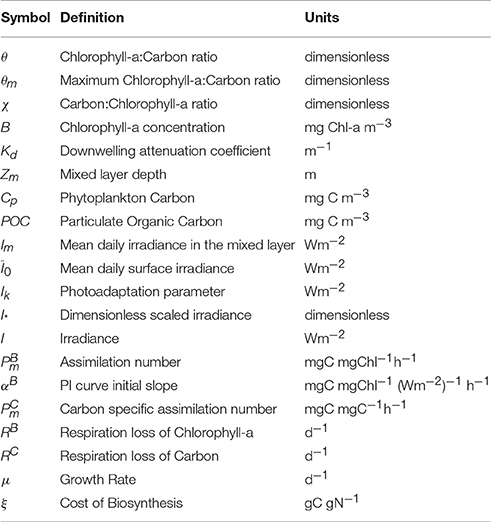
Table 1. Definitions of symbols.

The $P_m^B$ and α^B values allow the calculation of the photoadaptation parameter I_k, defined as $P_m^B/{\alpha }^B$. Surface Chl-a concentration from the Ocean Colour Climate Change Initiative (OC-CCI) dataset, Version 2.0 (European Space Agency, available online at http://www.esa-oceancolour-cci.org/) and the spectral light-transmission model of Sathyendranath and Platt (1988) were used to compute K_d, the diffuse attenuation coefficient for photosynthetically-active radiation for the mixed layer. The daily average irradiance in the mixed layer (I_m) was computed as

$\begin{array}{ll}{I}_m=\frac{{\overline{I}}_0}{K_d{Z}_m}(1-\text{exp}(-K_d{Z}_m)),& \left(2\right)\end{array}$

where ${\overline{I}}_0$ is the daily (24 h) average PAR at the sea-surface and Z_m is the mixed-layer depth (Platt et al., 1991; Cloern et al., 1995).

An in-situ bio-optical dataset of particulate organic carbon (POC), chlorophyll, and photosynthesis-irradiance parameters (Sathyendranath et al., 2009) was also used in this work. This dataset lacked information on PAR and MLD, which were filled in using the climatological data mentioned above.

3. Exact Solution for the Chlorophyll-to-Carbon Ratio (θ) in the Geider et al. (1997) Model

According to Geider et al. (1997), the chlorophyll-to-carbon ratio, θ, is a function of irradiance I:

$\begin{array}{ll}{\theta }^2={\theta }_{m}a\left(1-\text{exp}\left(-\frac{\theta }{a}\right)\right),& \left(3\right)\end{array}$

where (θ_m) is a prescribed model parameter, corresponding to the maximum attainable value of θ. The above equation is equivalent to equation A12 in Geider et al. (1997), noting that there is a typographical error in the equation, such that the denominator of the argument to the exponential term should be a, and not α^BI. For conditions of balanced growth, Geider et al. (1997) point out that their parameter k_chl, which represents the maximum proportion of photosynthesis that can be directed to chlorophyll-a synthesis, would be equivalent to the parameter θ_m. We have applied the equivalence here, such that the solution would be valid only for balanced growth. The model development also assumes that the specific respiration rates of carbon and chlorophyll are either negligible or equal to each other.

We note that $a=P_m^C/({\alpha }^{B}I)$, where $P_m^C$ is the carbon-specific, light saturated photosynthesis. By definition, $P_m^C=P_m^B\theta$, such that $a=P_m^B\theta /({\alpha }^{B}I)$. Substitution into Equation (3) gives:

$\begin{array}{ll}{\theta }^2={\theta }_{m}a\left(1-\text{exp}\left(-\frac{\theta {\alpha }^{B}I}{P_m^B\theta }\right)\right).& \left(4\right)\end{array}$

Applying the equivalence $I_k=P_m^B/{\alpha }^B$, we get

$\begin{array}{ll}{\theta }^2={\theta }_{m}a\left(1-\text{exp}\left(-\frac{I}{I_k}\right)\right),& \left(5\right)\end{array}$

and setting I/I_k = I_∗, a dimensionless irradiance, the equation becomes

$\begin{array}{ll}{\theta }^2={\theta }_m\frac{\theta }{I_{*}}(1-\text{exp}(-I_{*})).& \left(6\right)\end{array}$

Solution for θ is obtained by simplifying the equation above:

$\begin{array}{ll}\theta =\frac{{\theta }_m}{I_{*}}(1-\text{exp}(-I_{*})).& \left(7\right)\end{array}$

The solution expresses θ as a function I_∗, such that the chlorophyll-to-carbon ratio can be calculated explicitly as a function of the dimensionless scaled irradiance (I_∗). Note that the carbon-to-chlorophyll ratio χ = 1/θ. As I_∗ tends to zero, the exact solution (Equation 7) tends to θ_m. As I_∗ tends to infinity, the solution tends to zero. However, this limit for high values of I_∗ is approached very slowly, well beyond reasonable values of I_∗ that might be expected in the natural environment. The solution remains well-constrained for plausible values of I_∗.

We note that the same solution is obtained when, instead of substituting $P_m^C=P_m^B\theta$, we make the equivalent change of ${\alpha }_B={\alpha }^C/\theta$. The key to solution is consistency: both parameters have to be normalized to the same quantity, carbon or chlorophyll, it does not matter which. The solution is indifferent to the choice as (apart from θ) it contains only the dimensionless quantity I_∗. However, ecosystem models are often formulated to use carbon-normalized $P_m^C$ as input, along with α^B, in which case, Equation 7 becomes (see also Li et al., 2010):

$\begin{array}{ll}\theta =(({\theta }_m{P}_m^C)/(I{\alpha }^B\theta ))(1-\text{exp}((-I{\alpha }^B\theta )/P_m^C)).& \left(8\right)\end{array}$

In this context, θ can be retrieved from the above equation iteratively.

It is is also possible to calculate the sensitivity (relative) of θ to changes (relative) in I_∗; and we find

$\begin{array}{ll}\left|\left(\frac{d\theta }{\theta }/\frac{d{I}_{*}}{I_{*}}\right)\right|=\frac{\left(\text{exp}(-I_{*})(1+I_{*})-1\right)}{\left(1-\text{exp}(-I_{*})\right)}\le 1,& \left(9\right)\end{array}$

such that the relative error in θ will not be greater than that in I_∗.

3.1. The Approximate Solution

Geider et al. (1997) provided an approximate solution for θ using the first three terms of the Taylor expansion of exp(−θ/a):

$\begin{array}{ll}{\theta }^2={\theta }_{m}a\left(1-1+\frac{\theta }{a}-\frac{{\theta }^2}{2a^2}\right).& \left(10\right)\end{array}$

For comparison with the exact solution (Equation 7), we can rearrange terms in the approximate solution, such that it is also expressed as a function of I_∗. Following an initial simplification:

$\begin{array}{ll}{\theta }^2={\theta }_{m}a\left(\frac{\theta }{a}-\frac{{\theta }^2}{2a^2}\right);\theta ={\theta }_m\left(1-\frac{\theta }{2a}\right).& \left(11\right)\end{array}$

We can then substitute for $a=P_m^B\theta /({\alpha }^{B}I)$ to find

$\begin{array}{ll}\theta ={\theta }_m\left(1-\frac{I_{*}}{2}\right).& \left(12\right)\end{array}$

Geider et al. (1997) noted that the approximation holds for only for I_∗ < 1. This limitation is overcome by the analytic solution for θ (Equation 7), which is valid for all values of I_∗.

The approximate solution (Equation 12) and the exact solution (Equation 7) are identical and equal to θ_m as I_∗ tends to zero. But the approximate solution θ becomes zero when I_∗ = 2, and becomes negative for higher values. Hence the limitation with using the approximate solution for high values of I_∗.

3.2. Effects of Nutrients and Temperature

We see from the exact solution (Equation 7) that θ depends on $P_m^B$ through I_k. In the Geider et al. (1998) model, effects of nutrient limitation and ambient temperature on $P_m^B$ are accounted for, as follows:

$\begin{array}{ll}{P}_m^C=P_{ref}^C\frac{N}{N+K_N}f(T),& \left(13\right)\end{array}$

where $P_{ref}^C$ is the maximum C-specific rate of photosynthesis at a reference temperature, T is the ambient temperature, f(T) is the Arrhenius function, N is the nitrate concentration and K_N is the half saturation constant for nitrate uptake.

$P_m^B$, defined as $P_m^C\times \theta$, therefore contains implicitly the effects of temperature and nutrients on photosynthetic rates. Consequently, Equation 7 accounts for their effects on θ through $P_m^B$. Since $P_m^B$ is more readily measured in the field than $P_m^C$, the new solution facilitates the study of C:Chl ratio in the natural environment.

4. Results

4.1. Comparison between Exact and Approximate Solutions

4.1.1. Theoretical Comparison

The approximate solution (Equation 12) and the exact solution (Equation 7) for 1/θ = χ are shown in Figure 1 for three values of θ_m: 0.005, 0.01 and 0.02 (corresponding to carbon-to-chl ratios of 200, 100, and 50). For low values of I_∗ the exact and approximate solutions are practically indistinguishable from each other. But as I_∗ approaches and exceeds 0.8, the deviation between them becomes significant. For I_∗ close to 2.0 the approximate solution for θ tends to zero and the inverse of θ (the carbon-to-chlorophyll ratio, χ) tends to infinity, whereas the exact solution remains stable. Figure 1A shows that the absolute error is dependent on both θ_m and I_∗. However, the relative error (Figure 1B) is independent of θ_m. The approximation overestimates the carbon-to-chlorophyll ratio by around 15% when I_∗ = 0.8, by 50% at I_∗ = 1.235 and by 100% at I_∗ = 1.478.

FIGURE 1

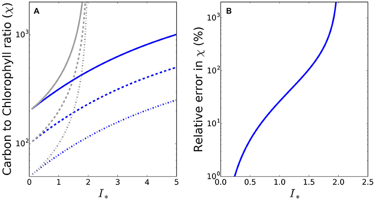
Figure 1. (A) The divergence of the approximate (gray) and exact (blue) solution estimates of the C:Chl ratio as a function of I_∗. Solid, dotted and dot-dash lines are for θ_m values of 0.005, 0.01, and 0.02 respectively. The exact solution is clearly stable across the full range of I_∗ values, while the approximate solution is not. (B) The relative difference between the approximate and the exact solutions as a function of I_∗.

4.1.2. A practical example

To see whether the differences between the exact and approximate solutions are likely to be significant under conditions encountered in the natural environment, we made some calculations at the global scale, using a combination of satellite and in situ data. The sequence of images in Figure 2 shows the input data fields (daily mean irradiance at the surface, mixed-layer depth, photoadaptation parameter I_k and chlorophyll-a concentration) and resultant daily mean irradiance in the mixed layer (I_m) and I_∗ for May 2010, where in this instance I_∗ = I_m/I_k. Of the valid ocean pixels in Figure 2F), 70.3% in the Northern hemisphere (which at the time would be the hemisphere of greater phytoplankton growth due to the spring bloom) have I_∗ values greater than 0.8, such that for these pixels the difference between the approximate and exact solutions would be greater than 15%. The error in the approximate solution is greater than 50% in some 24% of the Northern hemisphere pixels. During November a similar situation occurs in the Southern hemisphere, with I_∗ values greater than 0.8 in 61.5% of pixels (results not shown).

FIGURE 2

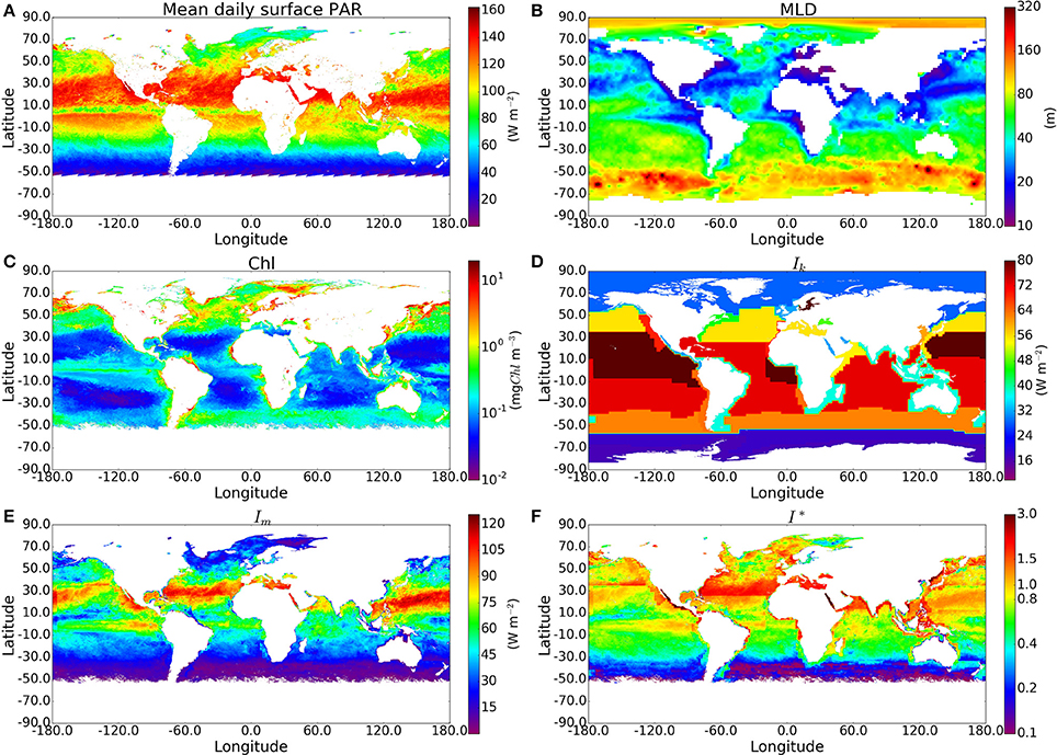
Figure 2. Map showing the input data and resulting I_∗ estimates at the global scale during May 2010. (A) SeaWiFS PAR product converted into W m⁻² (Morel and Smith, 1974) and averaged over the day (24 h), (B) MLD climatology (de Boyer Montégut et al., 2004), (C) OC-CCI v2.0 monthly composite of chlorophyll-a, (D) Biogeochemical-province based I_k (Mélin and Hoepffner, 2004), (E) daily-mean mixed-layer irradiance, and (F) daily-mean mixed-layer dimensionless irradiance. Values of I_∗ around 0.8 or greater (yellow and warmer colors) will give a significant difference between the approximate and exact solutions for C:Chl.

This demonstrates that phytoplankton in the surface oceans are frequently exposed to conditions in which the difference between the approximate and exact solution for θ is significant, and worth accounting for.

4.2. Computation of Phytoplankton Carbon in the Ocean

In this section, we first impliment the analytic solution using the in situ bio-optical data to compute phytoplankton carbon at the observation points. Since it is known that θ_m varies with phytoplankton type (Geider et al., 1997), we assigned values of θ_m according to phytoplankton size classes. First, based on the work of Brewin et al. (2010), the chlorophyll-a concentration at each data point was used to estimate the proportions of the three phytoplankton size classes (micro-, nano- and pico-plankton) present in the sample. Next, based on the C:Chl ratios given in Sathyendranath et al. (2009) for different phytoplankton types sampled in the natural environment, θ_m was set to 0.05, 0.02, 0.008 for micro-, nano- and pico-phytoplankton, corresponding to a minimum C:Chl ratio of 20, 50 and 125 for each size class. These values are consistent with θ_m values reported by Geider et al. (1997) for various phytoplankton species in culture and also by Li et al. (2010) in the natural marine environment. The θ_m for the populations was then computed as a weighted sum of the three components of the population. As θ_m dictates a maximum Chl:C ratio, it also sets a minimum C:Chl ratio. The photosynthesis-irradiance parameters ($P_m^B$ and α^B) in the database were then used to compute I_k (in situ) and the daily average I_∗ for the mixed layer, given the daily average I_m for the layer.

For each sample in the in situ dataset taken at a depth within the climatological mixed-layer depth (410 samples), we calculated the C:Chl ratio χ using I_∗ and θ_m, and then multiplied χ by the chlorophyll concentration measured in situ to estimate total phytoplankton carbon (C_p). Figure 3 shows measured POC plotted against computed phytoplankton carbon (C_p). The model imposes no upper limit on the C:Chl ratio. Therefore, if the model parameters were incorrectly assigned, it could lead to many C_p values being greater than the measured POC, which would clearly indicate an overestimation of phytoplankton carbon, since it should not exceed POC concentration. The C_p estimated using the analytical solution and estimated θ_m exceeds total POC in only 4 of the 410 points. Most of the C_p:POC ratios lie in the range of ≈10–70% with a mean of 31%, which is consistent with existing in situ measurements from the Atlantic and Pacific oceans (Martinez-Vicente et al., 2013; Graff et al., 2015), suggesting that θ values are not grossly underestimated either. The results using the approximate solution are significantly higher (I_∗ > 0.8 and difference >15%) in 130 of the 410 in situ measurements. The differences when using the in situ I_k values were greater than when the calculations were performed using the province-based average I_k values, demonstrating that sometimes, the errors from the approximate solution are reduced when using broadly-averaged fields of I_k, since averaging eliminates extreme values.

FIGURE 3

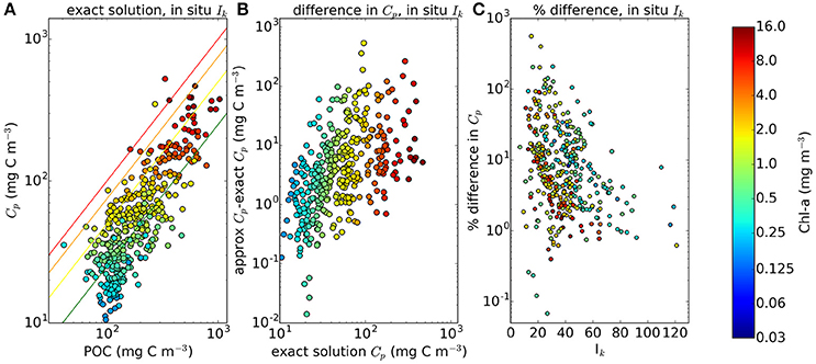
Figure 3. Comparison of phytoplankton Carbon estimates using the approximate and exact solution with in situ I_k data from around 400 samples, mostly from the N.W Atlantic region. (A) Calculated Phytoplankton Carbon (θ*B) in relation to POC measured for the BIO samples using the exact solution. Red, orange, yellow and green lines correspond to phytoplankton carbon equalling 100, 75, 50, and 25% of POC respectively. The θ_m values are calculated using an estimate of the community size structure calculated using the method of Brewin et al. (2010). (B,C) show the absolute and % difference between results from the exact and approximate solutions.

As the calculations yielded plausible values of phytoplankton carbon when compared with measured POC values, we applied the method to the I_∗ map and the satellite-derived chlorophyll field shown in Figure 2 to produce global maps of C:Chl ratio and C_p. The results are compared with the approximate solution to the Geider et al. (1997) model and with the method of Sathyendranath et al. (2009) (see Figure 4), which implemented the equation $C_p=64B^{0.63}$, where B is Chlorophyll-a concentration (see their Figure 1B). As expected, the C:Chl ratios from the exact solution are lower than those from the approximate solution, with the largest differences occurring in regions of high I_∗. The corresponding C_p values are also lower for the exact solution. The distribution of C_p values using the analytical solution appears more natural than those using the approximate solution, with fewer artificial boundaries present in the output fields.

FIGURE 4

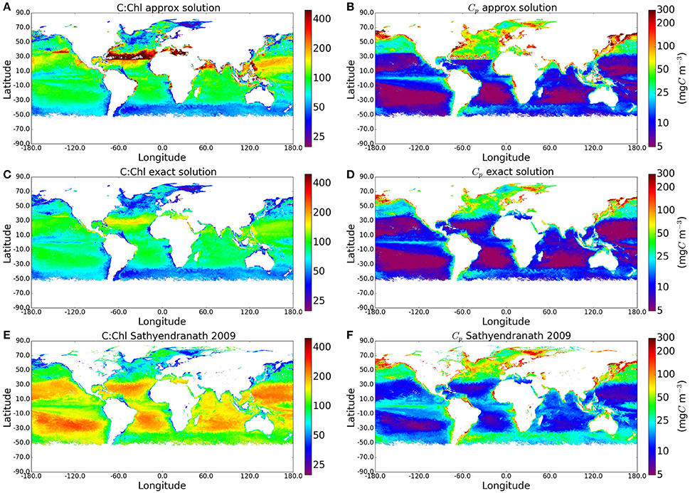
Figure 4. Maps comparing the C:Chl and C_p estimates using the original approxmiate solution, the new exact solution, and the method of Sathyendranath et al. (2009) globally for May 2010. The I_∗ and Chl input fields can be seen in Figure 2.

The exact solution for C_p is also closer (smaller mean absolute-difference) than the approximate one to the results from the empirical approach of Sathyendranath et al. (2009), but some of the similarities have to be attributed to the use of θ_m values from Sathyendranath et al. (2009) in this work. Both the exact solution and the method of Sathyendranath et al. (2009) show the anticipated increase in C:Chl ratio toward the subtropical gyres (associated with the dominance of pico-plankton in these areas), although the magnitudes differ. Similarly, in both these examples, the C:Chl ratio decrease toward the Southern Ocean. The similarities in patterns are encouraging. However, the exact solution provides a lower range for the C:Chl ratio globally, when compared with the outputs from the method of Sathyendranath et al. (2009). This is to be expected as the averaging of I_k by province and by season removes extreme values, as well as any small-scale variability that might otherwise be present in a dynamic assignment of I_k. On the other hand, we recognize that the method of Sathyendranath et al. (2009) is purely empirical and was designed to provide something of an upper limit to the carbon-to-chlorophyll ratio, whereas the Geider et al. (1997) model has a strong mechanistic basis and is able to account for the effects of photo-acclimation on θ. Clearly, more work is required to reconcile the differences between the empirical and theoretical approaches.

4.3. Application in Marine Ecosystem Models

In addition to the remote-sensing applications demonstrated above, the Geider et al. (1997) model is also used extensively in marine ecosystem models (Laufkötter et al., 2015). But to estimate the impact that the exact solution might have on the calculated fields of carbon-to-chlorophyll ratio, we have to consider the time scales over which light is averaged, before carbon-to-chlorophyll ratio is computed in the models. For example, in the European Regional Seas Ecosystem Model (ERSEM), the instantaneous light field is used to compute θ at each time step of the model (Butenschön et al., 2016). The common time step for ERSEM is 15 min. But other models, such as the “Darwin” model developed at MIT, perform these calculations at longer time steps (Dutkiewicz et al., 2015). A model with a 24 h time step might use daily-averaged light fields. Calculations that use short time-steps would have a greater range in I_∗ values, relative to those that use daily averages.

An example of a calculation of θ done at a 2-h time-step is shown in Figure 5, where results are plotted for optical depths of zero (surface) to 4. Note that one optical depth is the depth at which light is reduced to 1/e of the initial value, and that only 1% of the surface value remains at an optical depth of 4.6. In this example, we used a fixed I_k value of 50 Watts m⁻², and a noon-time maximum value of I at the surface of 400 W m⁻², and set θ_m = 0.01. The total daily irradiance was allowed to vary, over a 12-h day, as described by a sine function. At noon, I_∗ values of 1.0 or greater occur even down to the first optical depth and the errors in the approximate solution are high in the surface waters for a large portion of the day. The value of irradiance averaged over 24 h at the optical depth of 1 (dashed lines shown for comparison) is well below the peak values seen at noon; and as expected, the difference between the exact and approximate solutions is reduced, though still significant (over 20%), for this case. Even in this instance, the errors would increase toward the surface, as average light increased. This is consistent with the findings of Moore et al. (2006) that for surface populations, the peak irradiance can be significantly higher than the measured I_k.

FIGURE 5

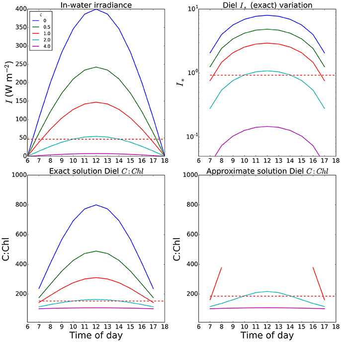
Figure 5. Variation in I_∗ and resultant C:Chl ratios through the a diurnal cycle at various optical depths in a simple optical model. The value set for I_k (50.0 W m²) was taken as a reasonable value from the fields seen in Figure 2. Both I_k and θ_m (0.01) were assumed uniform within a mixed layer extending to the euphotic depth. Dashed red lines show the value for the first optical depth when calculations are performed using a daily mean (24-h time step). Missing values in the final panel are due to values of I_∗ exceeding the limit of the Taylor expansion.

5. Discussion and Conclusion

In this paper we have presented a new, exact solution for the Geider et al. (1997) model for estimating the C:Chl ratio in phytoplankton as a function of a dimensionless irradiance scaled to the photoadaptation parameter, I_k. The result is directly applicable to remote-sensing and modeling of marine ecosystems, as demonstrated here, but finds further applications in modeling phytoplankton physiological properties, growth rates and stoichiometry (Sathyendranath et al., 2009; Dutkiewicz et al., 2015; Laufkötter et al., 2015). Using an in situ bio-optical database and the model, we have computed phytoplankton carbon, and shown that the derived ratios of phytoplankton carbon to POC were plausible.

The Geider et al. (1997) model was initially conceived to be implemented with $P_m^C$ and α^B as inputs. The work presented here provides a new exact solution to the model. The advantage of the solution is that it allows the Geider et al. (1997) model to be implemented in any instance where there are direct measurements or indirect estimates of I_k. So the starting point for implementation of the new solution would be estimates of I_k or $P_m^B$ and α^B. In this regard, the new solution takes the Geider et al. (1997) model in a new direction. However, in ecosystem models that are implemented with with $P_m^C$ and α^B as inputs, the value of θ can be found from the exact solution iteratively (note that Li et al., 2010 have also proposed a numerical solution). The extra computation required for an iterative solution would certainly be worth the effort, especially for I_∗ > 0.8, when errors in the approximate solution begin to be greater than 15% (Figure 1).

Irradiance is a fundamental driver of phytoplankton growth, and phytoplankton employ a suite of strategies in response to the range of irradiance conditions in the global oceans. Some groups of cyanobacteria have genetically diversified into “high-light” and “low-light” variants (Moore et al., 1998) taking advantage of the stable irradiance conditions in the central gyres. In more dynamic regions it is essential for algae to be able to respond to changes in the light environment. Here we have presented a refinement of the Geider et al. (1997) mechanistic model of carbon-to-chlorophyll ratio allowing a smooth response in phytoplankton C:Chl ratios across a greater range of irradiance conditions. This allows a more accurate calculation of model results across a complete range of spatial and temporal scales.

Geider et al. (1997) give two solutions for the Chl:C ratio, both for balanced growth. One of them assumes that the chlorophyll-a losses due to respiration are zero (R^B = 0) or that the chlorophyll-a specific degradation has the same dependence on specific growth rate as cellular carbon specific respiration (R^B = R^C = μξ, where μ is growth rate and ξ is the cost of biosynthesis). This is the option that has been pursued here, since it would be appropriate for use in models of gross primary production using photosynthesis-irradiance parameters that have already been corrected for respiration. If, instead, we were to use the model for the case where carbon respiration was not zero, an equivalent solution would exist, provided that a correction term were applied to θ_m as suggested by Geider et al. (1997). But, given the uncertainties in θ_m, and given that the correction term is typically found to be small, we can assume that the model discussed here is sufficient to cover such conditions as well, under our current state of knowledge. A more pertinent question is at what time scales the condition of balanced growth might be met. In fact, acclimation from one light level to another will take place over a finite period, with Geider et al. (1986) and Raven and Geider (2003) suggesting that the appropriate time scale for acclimation is of the order of hours to days, implying that balanced growth would hold on daily time scales. Moore et al. (2003, 2006) have provided examples where photoacclimation timescales were longer than those for surface mixing, and Talmy et al. (2013) highlighted the importance of surface irradiance, depth of mixing, and light attenuation using a resource allocation based model of photoacclimation. It is also apparent that when numerical models are run at short time steps (less than an hour), it will be increasingly important to account in some manner for non-balanced growth during the transition phase.

The solution for C:Chl can produce both high C:Chl values, in line with those exceeding 300 observed in cultures (Cloern et al., 1995), and the low values (25–70) observed in ocean samples (Riemann et al., 1989). That said, a suitable θ_m is essential to obtain the correct result. In the example presented here (Figure 3), a three-component model of phytoplankton size classes is used in the assignment of θ_m. Although this allows a dynamic estimation of θ_m it is still derived from fixed values for each group. Refinements in the estimation of θ_m would also result in improved estimates of the realized C:Chl values.

Our application of the model at large scales using remote-sensing data (Figure 2) utilized average estimates of I_k (by season and province), whereas in reality the values would be more variable. Dynamic assignment of parameters would lead to a greater range of I_∗ values, increasing the potential for errors when using the approximate solution for θ. The concept of dynamic estimates of photosynthesis parameters using environmental variables, has been discussed by Platt and Sathyendranath (1993, 1995), Saux-Picart et al. (2013), and Silsbe et al. (2016).

The computed carbon-to-chlorophyll ratio depends strongly on available light. It raises the question of what would be the appropriate value of I to use in the calculations, given that phytoplankton experience changes in available light over a variety of time scales. These include changes at time scales of seconds, as the sun rises and sets and as clouds pass, to seasonal scale changes dictated by the Earth's declination. In addition, phytoplankton are at the mercy of vertical movement of the water column due to, for example, turbulence, internal waves or upwelling. But what would be the appropriate time scales for acclimation of carbon-to-chlorophyll ratio? As noted above, previous studies have indicated that it is of the order of 1 day. But further information on this point would be valuable. A related matter, from a modeling perspective is that the photosynthetic response of phytoplankton to available light is instantaneous. So it is clear that computation of photosynthesis within numerical ecosystem models has to be driven by instantaneous light. If, along with such calculations, we need light fields averaged over some yet-to-be-defined time scale for computation of θ, simulation models would have to be designed to keep track of at least two values of available light, to be used as required. This time scale would be related to that appropriate for balanced growth, as discussed above.

The Geider et al. (1997) model presented here is re-formulated as a function of I_∗, which requires only the photosynthesis parameter I_k for implementation, in addition to data on available light. Bearing in mind the body of data on photosynthesis-irradiance parameters that exists, and the relative ease with which these parameters can be measured, compared with direct measurements of phytoplankton carbon in the field (see Casey et al., 2013; Graff et al., 2015), these results open up the possibility of significant augmentation of the information base on carbon-to-chlorophyll ratio in the marine environment. But when photosynthesis-irradiance parameters, available light and phytoplankton carbon are measured concurrently, we also have the possibility to estimate the parameter θ_m, about which we have so little information from the field.

Author Contributions

SS conceived the problem. TJ, SS, and TP worked jointly to find an analytical solution. TJ made all calculations and figures. The preparation of the manuscript was led by TJ with all authors contributing significantly to the final text.

Funding

This work was funded through the European Space Agency's MAPPS (MArine primary Production: model Parameters from Space) project as part of the Support to Science Element (STSE) Pathfinders Program and the POCO (Pools of Carbon in the Ocean) Project, which is a part of the SEOM (Scientific Exploitation of Operational Missions) Programme. This work is also a contribution to activities of the National Centre for Earth Observation (NCEO), UK. Additional support from Simons Foundation through the CBIOMES project is acknowledged. Finally the contribution of The Jawaharlal Nehru Science Fellowship to TP in the course of this work is gratefully acknowledged.

Conflict of Interest Statement

The authors declare that the research was conducted in the absence of any commercial or financial relationships that could be construed as a potential conflict of interest.

Acknowledgments

We thank ESA Ocean Colour Climate Change Initiative and NASA for the open-access remote-sensing products used in this work. We would like to thank all those who contributed to the in situ database used in this study, to Elizabeth Goult for performing sensitivity analysis checks. We thank Frédéric Mélin and Nicolas Hoepffner for making available their photosynthesis-irradiance parameter database for this work. We thank reviewers Christoph Voelker and Greg M. Silsbe for their helpful comments on the initial manuscript. We also thank Peter Regner and Diego Fernandez at ESA for their continuous support.

References

Brewin, R. J. W., Sathyendranath, S., Hirata, T., Lavender, S. J., Barciela, R., and Hardman-Mountford, N. J. (2010). A three-component model of phytoplankton size class for the Atlantic Ocean. Ecol. Model. 221, 1472–1483. doi: 10.1016/j.ecolmodel.2010.02.014

CrossRef Full Text | Google Scholar

Butenschön, M., Clark, J., Aldridge, J. N., Allen, J. I., Artioli, Y., Blackford, J., et al. (2016). Ersem 15.06: a generic model for marine biogeochemistry and the ecosystem dynamics of the lower trophic levels. Geosci. Model Develop. 9, 1293–1339. doi: 10.5194/gmd-9-1293-2016

CrossRef Full Text | Google Scholar

Casey, J. R., Aucan, J. P., Goldberg, S. R., and Lomas, M. W. (2013). Changes in partitioning of carbon amongst photosynthetic pico- and nano-plankton groups in the sargasso sea in response to changes in the north atlantic oscillation. Deep Sea Res. II Topic. Stud. Oceanogr. 93, 58–70. doi: 10.1016/j.dsr2.2013.02.002

CrossRef Full Text | Google Scholar

Cloern, J. E., Grenz, C., and Vidergar-Lucas, L. (1995). An empirical model of the phytoplankton chlorophyll:carbon ratio-the conservation factor between productivity and growth rate. Limnol. Oceanogr. 40, 1313–1321. doi: 10.4319/lo.1995.40.7.1313

CrossRef Full Text | Google Scholar

Cullen, J. J. (1982). The deep chlorophyll maximum: Comparing vertical profiles of chlorophyll a. Canad. J. Fish. Aquat. Sci. 39, 791–803. doi: 10.1139/f82-108

CrossRef Full Text | Google Scholar

Cullen, J. J. (2015). Subsurface chlorophyll maximum layers: enduring enigma or mystery solved? Annu. Rev. Marine Sci. 7, 207–239. doi: 10.1146/annurev-marine-010213-135111

CrossRef Full Text | Google Scholar

de Boyer Montégut, C., Madec, G., Fisher, A. S., Lazar, A., and Iudicone, D. (2004). Mixed layer depth over the global ocean: An examination of profile data and a profile-based climatology. J. Geophys. Res. 109:C12003. doi: 10.1029/2004JC002378

CrossRef Full Text | Google Scholar

Dutkiewicz, S., Hickman, A. E., Jahn, O., Gregg, W. W., Mouw, C. B., and Follows, M. J. (2015). Capturing optically important constituents and properties in a marine biogeochemical and ecosystem model. Biogeosciences 12, 4447–4481. doi: 10.5194/bg-12-4447-2015

CrossRef Full Text | Google Scholar

Frouin, R., Franz, B., and Werdell, P. (2002). The SeaWiFS PAR product. NASA Techn. Memorand. 2003 206892 22, 46–50.

Google Scholar

Geider, R. J. (1987). Light and temperature dependence of the carbon to chlorophyll a ratio in microalgae and cyanobacteria: implications for physiology and the growth of phytoplankton. New Phytol. 106, 1–34. doi: 10.1111/j.1469-8137.1987.tb04788.x

CrossRef Full Text | Google Scholar

Geider, R. J., Macintyre, H. L., and Kana, T. M. (1997). Dynamic model of phytoplankton growth and acclimation: responses of the balancedgrowth rate and chlorophyll a:carbon ratio to light, nutrient-limitation and termperature. Marine Ecol. Progr. Ser. 148, 187–200. doi: 10.3354/meps148187

CrossRef Full Text | Google Scholar

Geider, R. J., Macintyre, H. L., Kana, T. M., and Jan, N. (1996). A Dynamic Model of Photoadaptation in Phytoplankton. Limnol. Oceanogr. 41, 1–15. doi: 10.4319/lo.1996.41.1.0001

CrossRef Full Text | Google Scholar

Geider, R. J., Maclntyre, H. L., and Kana, T. M. (1998). A dynamic regulatory model of phytoplanktonic acclimation to light, nutrients, and temperature. Limnol. Oceanogr. 43, 679–694. doi: 10.4319/lo.1998.43.4.0679

CrossRef Full Text | Google Scholar

Geider, R. J., Platt, T., and Raven, J. A. (1986). Size dependence of growth and photosynthesis in diatoms: a synthesis. Marine Ecol. Progr. Ser. 30, 93–104. doi: 10.3354/meps030093

CrossRef Full Text | Google Scholar

Graff, J. R., Westberry, T. K., Milligan, A. J., Brown, M. B., Dall'Olmo, G., van Dongen-Vogels, V., et al. (2015). Analytical phytoplankton carbon measurements spanning diverse ecosystems. Deep Sea Res. I Oceanogr. Res. Papers 102, 16–25. doi: 10.1016/j.dsr.2015.04.006

CrossRef Full Text | Google Scholar

Halsey, K., and Jones, B. (2015). Phytoplankton strategies for photosynthetic energy allocation. Ann. Rev. Marine Sci. 7, 265–297. doi: 10.1146/annurev-marine-010814-015813

PubMed Abstract | CrossRef Full Text | Google Scholar

Hickman, A., Dutkiewicz, S., Williams, R., and Follows, M. (2010). Modelling the effects of chromatic adaptation on phytoplankton community structure in the oligotrophic ocean. Marine Ecol. Progr. Ser. 406, 1–17. doi: 10.3354/meps08588

CrossRef Full Text | Google Scholar

Laufkötter, C., Vogt, M., Gruber, N., Aita-Noguchi, M., Aumont, O., Bopp, L., et al. (2015). Drivers and uncertainties of future global marine primary production in marine ecosystem models. Biogeosciences 12, 6955–6984. doi: 10.5194/bg-12-6955-2015

CrossRef Full Text | Google Scholar

Li, Q. P., Franks, P. J. S., Landry, M. R., Goericke, R., and Taylor, A. G. (2010). Modeling phytoplankton growth rates and chlorophyll to carbon ratios in california coastal and pelagic ecosystems. J. Geophys. Res. Biogeosci. 115:G04003. doi: 10.1029/2009JG001111

CrossRef Full Text | Google Scholar

Longhurst, A. R., Sathyendranath, S., Platt, T., and Caverhill, C. M. (1995). An estimate of global primary production in the ocean from satellite radiometer data. J. Plankton Res. 17, 1245–1271. doi: 10.1093/plankt/17.6.1245

CrossRef Full Text | Google Scholar

Martinez-Vicente, V., Dall'Olmo, G., Tarran, G., Boss, E., and Sathyendranath, S. (2013). Optical backscattering is correlated with phytoplankton carbon across the atlantic ocean. Geophys. Res. Lett. 40, 1154–1158. doi: 10.1002/grl.50252

CrossRef Full Text | Google Scholar

Mélin, F., and Hoepffner, N. (2004). Global Marine Primary Production: A Satellite View. Ispra, VA: Institute for Environment and Sustainability.

Moore, C., Suggett, D., Holligan, P., Sharples, J., Abraham, E., Lucas, M., et al. (2003). Physical controls on phytoplankton physiology and production at a shelf sea front: a fast repetition-rate fluorometer based field study. Marine Ecol. Progr. Ser. 259, 29–45. doi: 10.3354/meps259029

CrossRef Full Text | Google Scholar

Moore, C. M., Suggett, D. J., Hickman, A. E., Kim, Y.-N., Tweddle, J. F., Sharples, J., et al. (2006). Phytoplankton photoacclimation and photoadaptation in response to environmental gradients in a shelf sea. Limnol. Oceanogr. 51, 936–949. doi: 10.4319/lo.2006.51.2.0936

CrossRef Full Text | Google Scholar

Moore, L. R., Rocap, G., and Chisholm, S. W. (1998). Physiology and molecular phylogeny of coexisting prochlorococcus ecotypes. Nature 393, 464–467. doi: 10.1038/30965

PubMed Abstract | CrossRef Full Text | Google Scholar

Morel, A., and Berthon, J.-F. (1989). Surface pigments, algal biomass profiles, and potential production of the euphotic layer: relationships reinvestigated in view of remote-sensing applications. Limnol. Oceanogr. 34, 1545–1562. doi: 10.4319/lo.1989.34.8.1545

CrossRef Full Text | Google Scholar

Morel, A., and Smith, R. C. (1974). Relation between total quanta and total energy for aquatic photosynthesis1. Limnol. Oceanogr. 19, 591–600. doi: 10.4319/lo.1974.19.4.0591

CrossRef Full Text | Google Scholar

Platt, T., Caverhill, C., and Sathyendranath, S. (1991). Basin-scale estimates of oceanic primary production by remote sensing: The north atlantic. J. Geophys. Res. Oceans 96, 15147–15159. doi: 10.1029/91JC01118

CrossRef Full Text | Google Scholar

Platt, T., Gallegos, C. L., and Harrison, W. G. (1980). Photoinhibition of photosynthesis in natural assemblages of marine phytoplankton. J. Marine Res. 38, 687–701.

Google Scholar

Platt, T., and Jassby, A. D. (1976). The relationship between photosynthesis and light for natural assemblages of coastal marine phytoplankton. J. Phycol. 12, 421–430. doi: 10.1111/j.1529-8817.1976.tb02866.x

CrossRef Full Text | Google Scholar

Platt, T., and Sathyendranath, S. (1993). Estimators of primary production for interpretation of remotely sensed data on ocean color. J. Geophys. Res. Oceans 98, 14561–14576. doi: 10.1029/93JC01001

CrossRef Full Text | Google Scholar

Platt, T., and Sathyendranath, S. (1995). “Latitude as a factor in the calculation of primary production,” in Ecology of Fjords and Coastal Waters, eds H. Skjoldal, C. Hopkins, K. Erikstad, and H. Leinaas (Amsterdam: Elsevier Science), 3–13.

Raven, J. A., and Geider, R. J. (2003). Adaptation, Acclimation and Regulation in Algal Photosynthesis (Dordrecht: Springer).

Google Scholar

Riemann, B., Simonsen, P., and Stensgaard, L. (1989). The carbon and chlorophyll content of phytoplankton from various nutrient regimes. J. Plankton Res. 11, 1037–1045. doi: 10.1093/plankt/11.5.1037

CrossRef Full Text | Google Scholar

Sathyendranath, S., and Platt, T. (1988). The spectral irradiance field at the surface and in the interior of the ocean: a model for applications in oceanography and remote sensing. J. Geophys. Res. 93, 9270–9280. doi: 10.1029/JC093iC08p09270

CrossRef Full Text | Google Scholar

Sathyendranath, S., Stuart, V., Nair, A., Oka, K., Nakane, T., Bouman, H., et al. (2009). Carbon-to-chlorophyll ratio and growth rate of phytoplankton in the sea. Marine Ecol. Progr. Ser. 383, 73–84. doi: 10.3354/meps07998

CrossRef Full Text | Google Scholar

Saux-Picart, S., Sathyendranath, S., Dowell, M., Moore, T., and Platt, T. (2013). Remote sensing of assimilation number for marine phytoplankton. Remote Sens. Environ. 146, 87–96. doi: 10.1016/j.rse.2013.10.032

CrossRef Full Text | Google Scholar

Silsbe, G. M., Behrenfeld, M. J., Halsey, K. H., Milligan, A. J., and Westberry, T. K. (2016). The cafe model: a net production model for global ocean phytoplankton. Global Biogeochem. Cycles 30, 1756–1777. doi: 10.1002/2016GB005521

CrossRef Full Text | Google Scholar

Talmy, D., Blackford, J., Hardman-Mountford, N. J., Dumbrell, A. J., and Geider, R. J. (2013). An optimality model of photoadaptation in contrasting aquatic light regimes. Limnol. Oceanogr. 58, 1802–1818. doi: 10.4319/lo.2013.58.5.1802

CrossRef Full Text | Google Scholar