Skipjack Tuna Availability for Purse Seine Fisheries Is Driven by Suitable Feeding Habitat Dynamics in the Atlantic and Indian Oceans

Introduction

Global annual catches of tropical and temperate tunas have been steadily increasing over recent decades, reaching 4.5 million tons (t) in 2015 (ISSF, 2017). Skipjack tuna (Katsuwonus pelamis, SKJ) currently accounts for about 60% of the annual global tuna catch, making it the third most fished species globally (FAO, 2014). In the Indian Ocean (IO), pole and line and gill net catches of SKJ increased from the 1950s onwards, reaching around 50,000 t by the end of the 1970s. When purse seine vessels arrived in the early to mid-1980s, catches rapidly increased on free swimming schools (FSC), peaking at around 615,000 t in 2006 (IOTC, 2016). During this time, drifting fish aggregating devices (dFADs) were increasingly deployed. These devices are known to attract a range of pelagic species including SKJ (e.g., Lopez et al., 2017). Now, fishers more commonly use artificial dFADs that they deploy and subsequently monitor using satellite-linked echo-sounders and precise positioning systems (Lopez et al., 2014). Since 2006, SKJ catches in the IO have decreased, varying between 340,000 t in 2012 and 440,000 t in 2008, with about 400,000 t caught in 2015. In the Atlantic Ocean (AO), SKJ catches also increased from the early 1950s and in recent years, have fluctuated around 230,000 t (ICCAT, 2016).

SKJ are a fast swimming pelagic fish that inhabit mostly tropical and sub-tropical waters. They are an opportunistic predator, mainly feeding on small fish species (including smaller SKJ), crustaceans and cephalopods (Magnuson, 1969; Roger, 1994; Allain, 2005). However, they are known to display regional dietary preferences (Mendizabal, 2013). They are the fastest growing tuna species, reaching around 45 and 65 cm fork length (FL) at age one and two, respectively (Murua et al., 2017). Their estimated maximum age is around 6–7 years old. SKJ oocyte development is asynchronous, meaning that oocyte recruitment is continuous over extended periods during which spawning occurs in multiple batches (Schaefer, 2001; Grande et al., 2012). In the IO, female SKJ length at 50% maturity (i.e., the length at which 50% of the female population is mature) is around 40 cm FL and full maturation is reached at about 50 cm FL (Stéquert and Ramcharrun, 1996; Grande et al., 2014). On average, their reproductive potential is large with around 1 million eggs produced per batch (Grande et al., 2014). SKJ are considered to be income breeders (Grande et al., 2016) meaning that the energy required for reproduction is mainly sourced directly from food intake, as opposed to accumulated energy reserves (McBride et al., 2015). This breeding strategy implies that higher investments in reproduction can be made when food resources are available (Kjesbu et al., 2009). Therefore, SKJ are characterized by fast growth and a spawning behavior that is strongly related to environmental conditions.

SKJ can perform extensive migrations. Large-scale tuna tagging programs conducted in the Eastern Pacific Ocean (e.g., Fink and Bayliff, 1970), Western Central Pacific Ocean (Kleiber et al., 1987; Hampton, 1997; Leroy et al., 2009, 2015) and IO (Murua et al., 2015) showed that on average, SKJ undertake horizontal migrations of more than 1,000 nautical miles (Fonteneau and Hallier, 2015). However, compared to other tuna species, their vertical movements are limited and restricted to surface waters. This is because they have a limited tolerance to low levels of dissolved oxygen and low temperatures (Graham and Dickson, 2004). SKJ exhibit high oxygen demands, notably because of their high metabolic rate, large red muscle mass and the absence of a swim bladder. These characteristics all facilitate SKJ's ability to make rapid vertical movements (Wild and Hampton, 1994). SKJ habitat is associated with a sea surface temperature (SST) range between 18 and 30°C (Barkley et al., 1978), with a preferred range between 23 and 28°C (e.g., Arrizabalaga et al., 2015). As SKJ have a limited ability to thermoregulate, suitable habitat is restricted to water masses that are relatively warm, have a high oxygen content and are close to cooler waters (below the thermocline) in order that they can release any excess metabolic heat.

Despite its economic importance, studies on SKJ habitat preferences are scarce, especially in the AO and IO. However, there is a considerable amount of purse seine data available for analysis that could offer interesting insights. Habitat analyses can range from a simple examination of the relationship between presence and SST (Andrade, 2003) to more complex investigations that derive SKJ feeding habitats as input data for spatial population models (using temperature and oxygen in APECOSM, Dueri et al., 2012; using a biogeochemical model in SEAPODYM, Lehodey et al., 1998). Using generalized additive models to associate SST, chlorophyll-a concentrations (CHL), sea surface height anomalies (SSHa), and eddy kinetic energy at weekly and monthly time scales, Mugo et al. (2010) undertook a more detailed analysis of SKJ habitat in the North Pacific Ocean. In this study, we used a rather different habitat modeling approach that uses daily chlorophyll-a fronts to track hotspots of pelagic productivity, in addition to physical environmental preferences. Therefore, it centers on the deterministic identification of productive fronts to detect prime areas of SKJ feeding habitat. We linked SKJ's ecological traits with environmental variables using an Ecological Niche Model approach (ENM) and investigated their feeding habitat requirements by analyzing presence and environmental data. Also known as species distribution modeling (Guisan and Thuiller, 2005; Elith and Leathwick, 2009; Peterson and Soberón, 2012), ENMs are a spatially-explicit method for modeling the ecological requirements of a given species and predicting its potential distribution in a geographical space. ENMs have many potential applications in ecological studies (see Guisan and Thuiller, 2005 for a review) but in the marine realm, they have mostly been used to examine invasive benthic species (e.g., Leidenberger et al., 2015; Marcelino and Verbruggen, 2015). Fewer studies have used them to consider pelagic species at fine time- and spatial-scales as their habitats are highly variable (Friedlaender et al., 2011; Druon et al., 2012, 2016). Having identified areas of favorable feeding habitat, we then calculated their distance from two types of fishing sets [free-swimming school sets (FSC) and drifting FAD associated sets (dFAD)] in both the AO and IO. This step was undertaken to (i) evaluate the links between habitat and fishing activity at both seasonal and decadal scales and (ii) examine the potential reproductive preferences of an incoming breeding species. Finally, we considered the benefits of using habitat modeling results in the context of dynamic fisheries management to support the sustainable exploitation of this resource.

Materials and Methods

Our ENM was composed of a five-step methodology (Figure 1) that aimed to: (1) identify the main behaviors and ecological traits of SKJ based on current literature and expert knowledge; (2) collect and process gridded data (presence-only and environmental variables) for defined study areas; (3) perform a cluster analysis to identify a set of variable thresholds that characterized SKJ feeding ecology; (4) derive the habitat model equation that classified the degree to which each portion (i.e., a model grid cell) of the study area was either suitable or unsuitable habitat (deterministic environmental envelope) on a daily basis; and (5) perform, by geographical area and fishing mode, a seasonal and inter-annual analysis using the distance of presence data to the closest favorable feeding habitat as a metric.

FIGURE 1

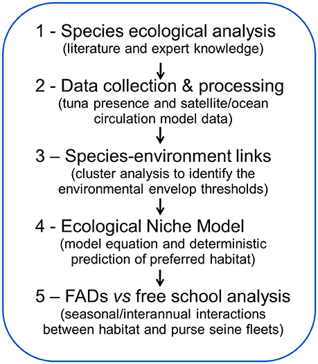
Figure 1. A flowchart of the Ecological Niche Model approach for skipjack tuna (Katsuwonus pelamis).

Step 1—From Skipjack Ecology to Habitat Trait

To begin, the ecological traits of SKJ that are known to influence its presence in the environment were identified. Tropical tunas species are known to generally aggregate in the vicinity of thermal fronts and temperate tuna species such as albacore (Thunnus alalunga) and Atlantic bluefin (Thunnus thynnus) have been shown to be attracted to chlorophyll-a fronts (Polovina et al., 2001; Royer et al., 2004; Druon et al., 2016). Chlorophyll-a fronts are a mesoscale feature that persist long enough (i.e., weeks to months) to sustain zooplankton production and thus, are known to attract upper trophic level species. As SKJ are both an opportunistic feeder and an income breeder (Grande et al., 2016), we hypothesized that SKJ are also attracted to these features. A time-lag between primary production and SKJ presence was not considered for these features as typically, these fronts frequently change shape and are in constant movement. Due to the scope of this study, we assumed that all productive fronts will attract higher trophic level species (including SKJ), however, in future work, it would be useful to estimate the age of the fronts. This age metric would provide useful insights into the likely stage of development in the aggregated food chain. Instead, in this study, we used the horizontal gradient of chlorophyll-a (gradCHL) as a proxy for food availability and the primary index of SKJ feeding habitat. We also used specific chlorophyll-a concentrations (CHL) as a secondary proxy for favorable feeding habitat. This is because SKJ are known to locate their prey by sight and thus, avoid waters with high CHL (Nakamura, 1968). Given that SKJ's limited tolerance of temperature restricts their distribution to surface waters (e.g., Barkley et al., 1978, see also section Introduction), a specific SST range was introduced into the habitat model. Sea surface height anomalies (SSHa) were another variable we identified as impacting the distribution of favorable feeding habitat (Mugo et al., 2010). SSHa is mainly influenced by seasonal changes in temperature and the geostrophic currents that characterize eddies and gyres i.e., areas of divergence and convergence. These features are commonly associated with enhanced primary productivity and thus, prey aggregation (Polovina et al., 2006; Benitez-Nelson et al., 2007; Tew Kai and Marsac, 2010; Bakun, 2013). Tropical tunas live in warmer, less productive environments that display near null or positive SSHa values whereas temperate tuna species are associated with negative SSHa values (Teo and Block, 2010; Arrizabalaga et al., 2015; Lopez et al., 2017). Sea surface salinity (SSS), sea surface current intensity (SSC), sea surface dissolved oxygen (O₂), and mixed layer depth (MLD) also have been shown to affect SKJ distribution at different spatio-temporal scales (Dizon, 1977; Barkley et al., 1978; Evans et al., 1981; Lopez et al., 2017, see also section Introduction) and were also included in our analysis.

Step 2—Data

Skipjack Tuna Presence-Only Data

In this study, SKJ presence data points were defined as purse seine sets in which SKJ was identified, regardless of its quantity or proportion to other species. Presence data was obtained from European Union (EU) tropical tuna purse seine fleet logbooks operating in the AO and IO. A total of 155,064 SKJ presence-only data points (with precise Global Positioning System locations—GPS) were collected for the Spanish fleet (1997–2014) and French fleet (1997–2015) (Figure 2). Redundancy filtering ensured that observations collected on the same day were separated by more than 2.3 km i.e., about half the width of a model cell.

FIGURE 2

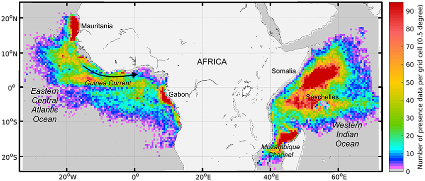
Figure 2. The geographical density of skipjack tuna (Katsuwonus pelamis, SKJ) presence data for both free-swimming schools and drifting fish aggregating device associated schools (n = 155,064) collected between 1997 and 2015 by European purse seine fleets (in number of observations by 0.5 degree grid cell). Density quartiles (i.e., 25^th, 50^th, and 75^th percentiles) per grid cell are 4, 12, and 30 and the 95^th percentile is 95.

Chlorophyll-a Data

Daily CHL (mg.m⁻³) data were obtained from SeaWiFS (1998–2010; 1/12° resolution) and MODIS-Aqua (2003–2015; 1/24° resolution) ocean color sensors using the OCI algorithm (Hu et al., 2012). Both products were extracted from the NASA portal (https://oceancolor.gsfc.nasa.gov/cgi/l3). Using this data at a daily time scale, meso-scale CHL fronts were identified. Daily CHL data were pre-processed using iterations of a median filter in order to recover missing data on the edge of the valid data, followed by a Gaussian smoothing procedure (see Druon et al., 2012 for details). Chlorophyll-a fronts were derived from the daily CHL data using an edge-detection algorithm. This approach was shown to perform better than the histogram methods for detecting horizontal gradients, given clear viewing conditions (Ullman and Cornillon, 2000). In the equatorial area of the Eastern Central AO, we encountered particularly poor data coverage due to cloud presence. This generated a substantial bias in the estimated habitat size derived from the multi-annual time series that we calculated using a combination of both data products. To address this problem and ensure temporal consistency, we used the SeaWiFS and MODIS-Aqua data separately in the AO to generate independent time-series of habitat size.

Abiotic Oceanographic Data

Data for the abiotic variables [i.e., SSHa (m), SSC (m.s⁻¹), SST (°C), SSS (PSU), and O₂ (mmol.m⁻³)] were extracted from the global ocean model (1997–2014) provided by the EU Copernicus Marine Environment Monitoring Service (http://marine.copernicus.eu/). Monthly mean data were extracted from the global model (Glorys2V3) with a 1/4° horizontal resolution and 75 unevenly spaced vertical levels. This ocean model includes a variational data assimilation scheme for vertical temperature and salinity profiles and satellite sea level anomalies (Oddo et al., 2009). These monthly data were interpolated onto the MODIS-Aqua grid (1/24° resolution) and then linearly interpolated to obtain daily values that matched the SKJ sampling day. This month-to-day interpolation step was assumed to produce suitable estimates of the seasonal changes that define SKJ habitat. SST and SSS values were calculated from the upper model layer (ca. 3 m) and thus, considered to be representative of the mixed layer. MLD was defined as the maximum of the vertical density gradient which was derived from the temperature and salinity profiles. SSC values were calculated from the mean value of the upper four layers of the ocean model (ca. 13.5 m) in order to account for current intensity and the eventual transport of the surface layer. SSC was included in the habitat model as a directionless quantity. O₂ values were calculated as the mean value of the upper 28 m of the ocean model (fifteen upper layers) to account for conditions of reasonable habitat size in the vertical dimension.

Step 3—Characterization of SKJ Feeding Habitat

In step three, we considered the environmental variability of each covariate, with a view to identifying the threshold values that characterize favorable vs. unfavorable feeding habitat. These analyses were carried out using the 1997–2014 abiotic data and the 1998–2015 CHL data.

The links between each environmental variable and tuna presence were analyzed for each ocean basin using cluster analysis (Hartigan, 1975; Berthold et al., 2010). The cluster analysis approach is particularly well suited for identifying habitats that are marginally represented by the data and may otherwise be interpreted as outliers by other statistical methods. In our analysis, we used daily or 3-day mean values of CHL and gradCHL and daily interpolated values from monthly means for SST, SSS, MLD, O₂, SSC, and SSHa. The CHL and gradCHL data were both log-transformed prior to use due to the wide variability in their values. All the variables were normalized by the mean and standard deviation [(x - mean)/deviation] prior to performing the cluster analysis. We performed two separate analysis, one using the biotic (CHL and gradCHL) variables and the second using the abiotic variables. This ensured that the number of points in each analysis were maximized since the CHL data were more infrequent (due to cloud-cover) than the always-defined abiotic data.

Cluster analysis is a suitable method for identifying homogenous groups of objects or “clusters” (in this instance, favorable SKJ habitats), regardless of their respective number. In presence data sets, a particular habitat is often over-represented but a cluster analysis allows under-represented environments to be identified. To ensure we represented the largest possible environmental envelope for SKJ, we used boundary values from the extreme clusters. For the abiotic variables, this meant that we used the 5^th percentile value of the lower cluster and the 95^th percentile value of the upper cluster, thus ensuring that any under-represented environments in the presence data were properly accounted for.

For the biotic thresholds, we excluded the cluster that showed very low levels of gradCHL (i.e., no CHL fronts), in line with our hypothesis that feeding opportunities are associated with CHL fronts. Thus, clusters needed to show at least a medium level of gradCHL to be considered to define preferred feeding habitat. Compared to the abiotic variables, we selected less stringent thresholds for the biotic variables (i.e., the 15^th, 20^th, and 85^th percentile values), in line with those chosen for other studied species (Druon et al., 2015, 2016). These thresholds were chosen to reflect the fact that while tunas are hypothesized to often occur in the vicinity of productive fronts, they will not necessarily occur at the fronts' exact location (Sund et al., 1981; Fiedler and Bernard, 1987; Mugo et al., 2014). Again, these thresholds were selected to ensure that the extremities of the environmental boundaries were represented but the distribution tails of the extreme clusters rejected. These tails likely correspond to outliers, for example, unusual environments, possible errors in the presence data or misclassified data in the clustering.

Step 4—Formulation of the Ecological Niche Model

Once the environmental variables were selected and the relevant threshold values set, the specific feeding habitats of SKJ were identified. These were defined as the common areas between favorable biotic conditions and abiotic preferences. The favorable environmental envelope predicted the daily suitability of each grid cell as a feeding habitat, assigning a binary habitat value (i.e., 0 or 1) for each biotic and abiotic variable, depending on whether its value was outside (0) or inside (1) the relevant favorable range. A continuous value between 0 and 1 was applied to gradCHL as large CHL fronts are more resilient and more likely to generate higher zooplankton biomasses than small CHL fronts (see Supplementary Information for more details). The areas that met the daily biotic and abiotic requirements of the habitat model were then integrated over time to create seasonal feeding habitat suitability maps, expressed as a frequency of occurrence (i.e., the sum of the daily habitat values [from 0 to 1] over the number of days for which the habitat was effectively estimated).

Step 5—Comparison between Fishing Activity and Feeding Habitat

Model performance was estimated by computing the distances between the presence data and the closest favorable feeding habitat (as defined by the 3-day mean composite data) for the period between 1998 and 2014. We then compared the distribution of these distances between the two fishing modes and ocean basins. A more detailed monthly analysis of these distances was also performed to investigate seasonal links between the number of fishing sets and the size of the favorable feeding habitat.

Mean annual SKJ catch rates (t.d⁻¹) were computed for the EU and associated purse seine fleets as the ratio between annual catch and annual fishing effort (expressed in fishing days; Chassot et al., 2015). Temporal correlations between annual catch rates and favorable feeding habitat size were investigated at the ocean basin scale using Spearman's rank correlation coefficients. Two independent time-series of habitat size were derived in the AO using SeaWiFS (1998–2010) and MODIS-Aqua sensors (2003–2014). This was done to avoid the bias that arose from differences in habitat coverage within the common period (i.e., 2003–2010) due to considerable cloud cover in the equatorial area.

Results

Habitat Modeling and Parameterization

SKJ can occur in a broad range of biotic and abiotic oceanographic conditions. However, in this study we assumed that given SKJ is an income breeder, it will always tend to seek out favorable feeding grounds. Thus, except during brief migrations periods, SKJ presence can be used to identify the existence of nearby favorable feeding habitat. The cluster analysis described a wide range of suitable trophic conditions for SKJ to feed, from the oligotrophic conditions in some regions of the Western IO and equatorial AO to the eutrophic conditions in the upwelling areas of the tropical AO (Table 1, Figures SI-2, SI-3). The threshold values for CHL and gradCHL were found to be of the same order of magnitude between the MODIS and SeaWiFS data and the differences are likely attributable to differences in data resolution and the optical characteristics of the sensors. The favorable CHL range was found to be between about 0.12 and 5 mg.m⁻³ in both oceans while the minimum and intermediate gradCHL values were found to be around 7.10⁻³ and 5.10⁻² mg.m⁻³.km⁻¹, respectively. Due to the cloud coverage in both oceans, <18% of the presence data could be associated with the closest 3-day (±1 day of the observation) composite favorable feeding habitat for CHL and 14% for gradCHL. For SST and SSS, favorable feeding habitat was characterized by the relatively large ranges of 21.6–30.0°C and 30.3–36.2 PSU, respectively. The SSHa distribution that describe 90% of the presence data ranged from a minimum of −0.2 m (in the AO) to a maximum of 0.67 m (in the IO) while the MLD range was 6–158 m. Finally, the minimum O₂ value observed was 196 mmol.m⁻³ (4.4 ml.l⁻¹).

TABLE 1

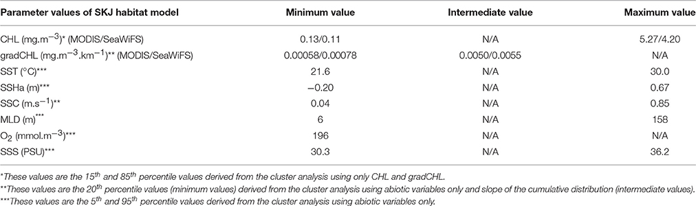
Table 1. Model parameters used to define favorable feeding habitat for skipjack tuna (Katsuwonus pelamis, SKJ) in the Eastern Central Atlantic and Western Indian Oceans (see also Figures SI-2, SI-3, SI-5) where SST (sea surface temperature), SSHa (sea surface height anomalies), SSC (sea surface current intensity), MLD (mixed layer depth), O₂ (sea surface dissolved oxygen), and SSS (sea surface salinity).

Outputs of the Habitat Model

Seasonally, favorable feeding habitat size and EU purse seine fleet activity levels varied among years (Figure 3). The years and seasons presented in this section were specifically selected to highlight differences in habitat size and fishing activity we observed between the 2000s and 2010s. In the AO, FSC sets were mostly located in the upwelling areas off Mauritania and Gabon in both the 2000s and 2010s (Figures 3A–D). To a lesser degree, they also occurred in the Guinea Current in the 2000s from November to March (Figure 3A). In contrast, dFAD sets in the 2000s generally occurred in the equatorial region, away from the upwelling areas (Figures 3A,B), except for the period August to October. During the 2010s, dFAD fishing was also pronounced between November and March in the Guinea Current (Figure SI-1). In both decades, most sets (FSC and dFAD) made between July and September (i.e., period when favorable feeding habitat was at its largest) occurred in upwelling areas (Figures 3B,D). In general, the favorable feeding habitats showed low latitudinal variability between the seasons but large winter-summer contraction-relaxation cycles. An unusual absence of favorable habitat was observed south of the equator during the 2002–2003 winter due to exceptionally high levels of salinity i.e., above 36 PSU (Figure 3A).

FIGURE 3

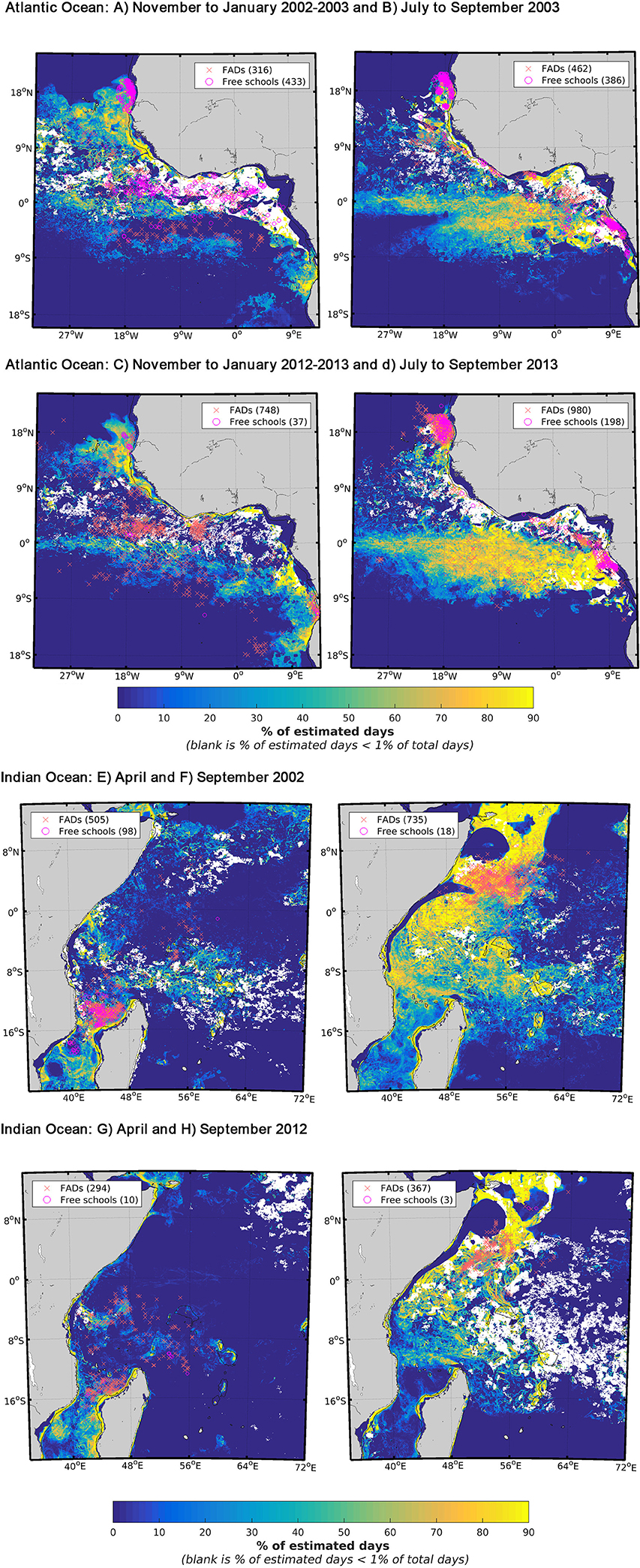
Figure 3. Seasonal favorable feeding habitat and fishing activity defined by presence fishing sets on skipjack tuna (Katsuwonus pelamis) in the Eastern Central Atlantic between (A) November and January 2002–2003, (B) July and September 2003, (C) November and January 2012–2013, (D) July and September 2013 and in the Western Indian Ocean between (E,F) April and September 2002 and (G,H) 2012. The drifting fish aggregating device associated sets (dFAD) presence data (red crosses) and the free-swimming school sets (pink circles) were overlaid with their respective numbers of presence data. The monthly ranges and years presented in these figures were chosen specifically to show stark contrasts in terms of fishing mode and habitat size i.e., small (A,C,E,G) vs. large (B,D,F,H). Favorable feeding habitat is defined by the presence of favorable environmental variable values and expressed as a frequency of occurrence. The blank areas correspond to habitat coverage below 1% of the total number of days in the considered time period.

In the IO, the presence of favorable feeding habitats and fishing grounds were highly seasonal, with an extended area of habitat observed in the northern region (especially off Somalia) from July to February (Figures 3F,H). Conversely, a restricted area of habitat with concentrated fishing effort was observed to typically occur in the Mozambique Channel in April (Figures 3E,G). In the IO, the proportion of dFAD sets in which SKJ were present was always above 80% between 2002 and 2012 and over 90% after 2008 (Figure SI-1).

The monthly area of available favorable feeding habitat (line segments) and the number of positive sets for which habitat information was available (width of boxes) were highly seasonal (Figure 4). In the AO (Figure 4A), 61% of FSC sets were made within a favorable feeding habitat while 16% were made more than 100 km away (n = 2,447). For dFAD sets, 34% were made within a favorable feeding habitat while 34% were made more than 100 km away (n = 3,159; Table 2 and Figure 5). In general, most AO-FSC sets were made within a short distance of favorable feeding habitat and during the months when this habitat was at its smallest (October–May, Figure 4A, upper graph) in the upwelling areas (Figures 3A–D). An exception to this pattern was observed between February and March in 2004 and 2009. For AO-dFAD sets, the longest distances from favorable feeding habitats were mainly observed between December and March (Figure 4A, lower graph). This time period is also when favorable habitat was at its smallest. These mostly corresponded to dFAD sets made in the Guinea Current (Figures 3A,C). The mean size of favorable feeding habitat varied from about 9% of the study area between January and April to around 17% in August (Figure 4A).

FIGURE 4

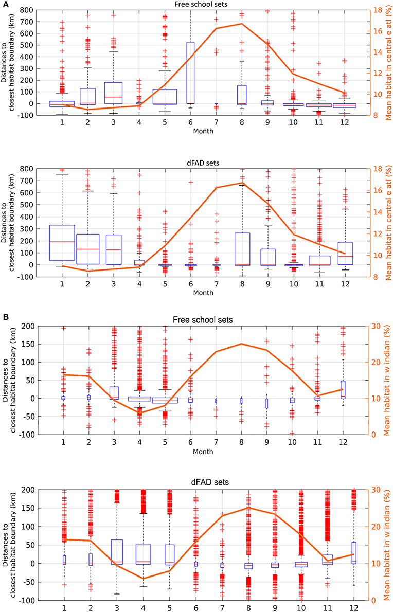
Figure 4. Monthly boxplots of the distances between skipjack tuna (Katsuwonus pelamis; SKJ) presence data and the closest favorable feeding habitat boundary for free-swimming school sets (FSC; upper panels) and drifting fish aggregating device associated sets (dFADs; lower panels) in (A) the Eastern Central Atlantic Ocean and (B) the Western Indian Ocean from 1998 to 2014. Negative values correspond to presence data points observed inside the favorable feeding habitat. The width of the boxes is proportional to the monthly number of sets while the box length corresponds to the interquartile range (median value in red, whiskers cover 99.3% of data if normally distributed, red crosses are outliers). The monthly sizes of favorable feeding habitats were overlaid (right axis, mean fraction of ocean area).

TABLE 2

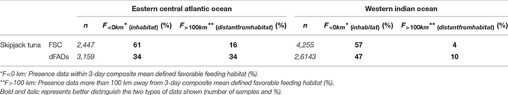
Table 2. Proportion of presence data within favorable feeding habitat and more than 100 km away, by ocean basin and fishing mode (%).

FIGURE 5

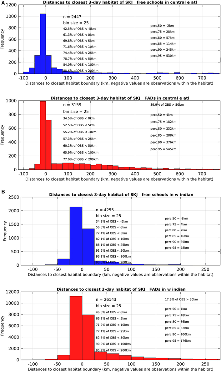
Figure 5. Detailed histograms and statistics of relating to the distances observed between skipjack tuna (Katsuwonus pelamis; SKJ) presence data (free-swimming school set (FSC) data shown in the upper blue graph and drifting fish aggregating device associated sets (dFAD) shown in the lower red graph) to the closest favorable feeding habitat boundary in (A) the Eastern Central Atlantic Ocean and (B) the Western Indian Ocean. Negative distance values correspond to presence data points observed within the favorable feeding habitat. Note the different ranges on the x-axis between the two study areas.

In the IO, the calculated distances from favorable feeding habitat were substantially lower for both fishing modes. For FSC sets, 56% were made within a favorable feeding habitat and only 4% were made more than 100 km away (n = 4,255). For dFAD sets, 47% were made within a favorable feeding habitat, while 10% were made more than 100 km away (n = 26,143; Figure 5). A marked inverse relationship between the number of sets (width of boxes in the boxplot) and habitat size was observed in the IO. Here, most of the FSC sets were made from March to May and most of the dFAD sets were made from March to May and October to November. These times corresponded to periods of minimum habitat size (about 5–10% of the study area compared to the maximum 15–25%, Figure 4B).

Overall, in both oceans, 83% of FSC sets (n = 6702) and 75% of dFAD sets (n = 29302) were found within 25 km of a favorable feeding habitat (Figure 5). In comparison, 8% of FSC sets (n = 557) and 13% of dFAD sets (n = 3691) were made more than 100 km away. These longer distances were mostly observed in the poor environment of the Guinea Current in the AO and during seasonal transitions in habitat in the IO.

In the AO, the favorable feeding habitat size showed substantial year-to-year variability (up to 22%) but we didn't observe any overall habitat trends, despite a tripling of catch rates and a doubling of total catch recorded for the same period (Figure 6A). The fraction of total catches (in weight) made up by EU fleet dFAD sets in this area increased from 50 to 75% prior to 2005 to 88–93% after 2006.

FIGURE 6

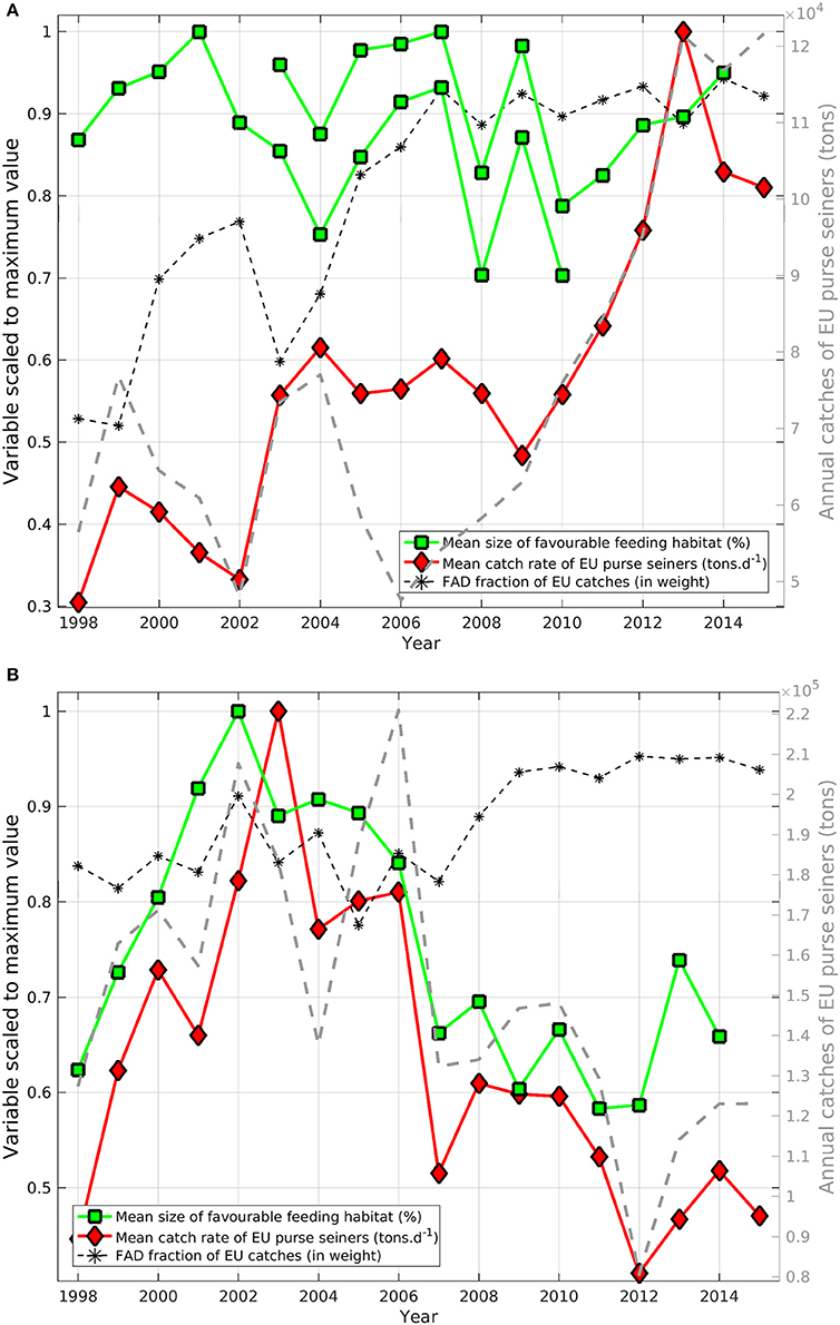
Figure 6. Annual indices of habitat size (green squares) and catch rate (red diamonds) of skipjack tuna (Katsuwonus pelamis; SKJ) scaled to the maximum values in the time-series of total catches (dashed gray line, tons, right axis) in (A) the Eastern Central Atlantic Ocean and (B) the Western Indian Ocean. The proportion of dFAD catches (in weight; black stars) is overlaid (%, left axis). To avoid issues associated with cloud coverage, two independent time-series of annual favorable feeding habitat size were derived for the Atlantic using SeaWiFS (1998–2010) and MODIS-Aqua (2003–2014) data.

In comparison, annual catch rates and favorable feeding habitat size showed clear trends and variations in the Western IO (Figure 6B). From 1998 to 2003–2004, habitat size increased 38% while catch rates increased 56%, However, from 2003 to 2004 onwards, habitat size decreased 42% while catch rates decreased 57%. In the IO, favorable feeding habitat size and catch rates were significantly correlated with a Spearman's rank correlation coefficient of 0.8 (p < 0.001). Despite probable differences in fishing effort and fishing efficiency, total catches also showed substantial correlation with feeding habitat size (r = 0.7, p < 0.001). Habitat size, catch rates and total catches showed markedly lower levels from 2007. From 2009 onwards, the fraction of SKJ caught (in weight) on dFAD sets made by the EU fleet showed an overall increasing trend, rising from about 85% to about 95% of total purse seine catches.

Discussion

Modeling Methods

The application of a common model parameterization across ocean basins and the substantial volume of data used in this study enabled us to successfully identify the ecological niche of SKJ in the Eastern Central AO and Western IO. In this study, we were fortunate enough to obtain presence data that covered a wide geographical extent and data for an extensive range of environmental conditions. Moreover, relatively long time-series (1998–2014/2015) were available for these data sets. This allowed us to derive a robust ENM for SKJ. We assumed that large productive fronts are more resilient than smaller features and thus, more able to sustain well-developed food chains on which SKJ can feed (Olson et al., 1994). Thus, in this study, the linear function linking daily favorable feeding habitat values with the size of gradCHL values provided an estimate of feeding capacity across productive fronts of differing sizes.

In order to identify and set the model parameterization, we conducted separate cluster analysis on the biotic and abiotic variables. We undertook these analyses separately because there were fewer CHL-related data points available (a 2.5-fold difference in the IO and an 8-fold difference in the AO) than data for the abiotic variables. The use of a cluster analysis that combined both sets of variables would not have accounted for as much abiotic variability. By using a clustering method, we ensured that environmental characteristics that may be important for SKJ but under-represented in the presence data were captured. This was essential for correctly identifying their overall ecological niche. Furthermore, the model parameterization excluded the biotic cluster that represented near-null gradCHL values to ensure that the resultant habitat, in combination with the abiotic preferences (established from the cluster analysis of the abiotic variables), only described the feeding behavior.

Habitat Characteristics of Skipjack Tuna and Their Ecological Role

The common feeding niche identified for SKJ emphasized the highly contrasting oceanographic regimes across the two ocean basins. In the IO, the seasonal occurrence of eddy-type mesoscale productive features were observed whilst in the AO, large scale upwelling systems that shrink and swell seasonally due to the influence of trade wind systems in the boreal summer periods were noted (Herbland et al., 1983; McGlade et al., 2002). The threshold ranges we identified through the cluster analysis for our environmental variables were consistent to those reported in field observations (e.g., Lopez et al., 2017) although the latter often refer to near lethal levels rather than preferences. The preferred SST range we identified (21.6–30.0°C) is nearly identical to the extreme SST range measured at-sea by the French purse seine fleet at SKJ set locations (21.5–30.0°C; IRD, unpublished data). A similar range was also obtained from the fishery-independent (Lopez et al., 2017) and fishery-dependent based preference models developed for SKJ (Andrade, 2003; Arrizabalaga et al., 2015; Tanabe et al., 2017). For O₂, Barkley et al. (1978) found that a minimum value of 3–3.5 ml.l⁻¹ (134–156 mmol.m⁻³) was necessary for the long-term survival of SKJ while Arrizabalaga et al. (2015) found that a value around 3.8 ml.l⁻¹ (170 mmol.m⁻³) was preferred by for SKJ across the world's oceans. Here, we found that the minimum preferred value was 4.4 ml.l⁻¹ (196 mmol.m⁻³) which is consistent with previous findings, noting that the present study area is smaller and in this case, the threshold relates to preference not survival. The preferred range for MLD ranged from 6 to 158 m and is consistent with the distributions found by Arrizabalaga et al. (2015) and Tanabe et al. (2017). Our observed minimum limit appears to be near the extreme observed level. The preferred SSC distribution compiled by Arrizabalaga et al. (2015) for the world's oceans (ca. 33.0–37.2 PSU) was different to the values we observed (30.3–36.2 PSU). The lower minimum value obtained in this study was driven by the large number of fishing sets in the Gabon upwelling where salinity levels are particularly low (Longhurst and Pauly, 1987). Arrizabalaga et al. (2015) global range for SSHa (ca. −0.4 to 0.8 m) was slightly broader, but nonetheless consistent with our findings (−0.20 to 0.67 m) given that our study area was smaller.

In both oceans, about 12% of all SKJ sets with suitable habitat coverage were located more than 100 km away from a favorable feeding habitat. We also noted differences in these distances between fishing modes and ocean basins. Distant sets (beyond 100 km) were proportionally, four times more frequent for FSC sets and more than three times more frequent for dFAD sets in the AO, compared to the IO. The apparent latitudinal migration of SKJ in the IO matched the transition periods between the peaks of productivity predicted by the habitat model off Somalia (July–November) and in the Mozambique Channel (April). We also noted an agreement with the spatial seasonality of EU purse seine fleet activity in the IO (Davies et al., 2014). In the AO, although fishing sets coincided with favorable feeding habitat within upwelling areas, there was no relationship in the Guinea Current. Here, the peak number of dFAD sets occurred from December to March, a period characterized by the absence of productive fronts, high SSTs, high SSHas and low O₂ levels. These variables are representative of poor feeding conditions compared to the upwelling areas (Pérez et al., 2005). It appears that some SKJ may migrate from productive and relatively cool upwelling areas to the poorer and warmer equatorial waters (see apparent movements by conventional tagging in Bard, 1986; ICCAT, 2014). Although, SKJ are known to spawn opportunistically year-round (Grande et al., 2014), we hypothesize that the Guinea Current may represent a preferred nursery area, as these environmental conditions favor larval survival (i.e., thermal stability and the lower presence of predators). In particular, we noticed that the SST ranges associated with most of the sets made in the Guinea Current (i.e., 5–95^th percentile values of 25.2–29.4°C) had little overlap with the SST ranges associated with sets made in the upwelling areas (Mauritanian values are 21.6–25.9°C and Gabon values are 22.6–27.7°C). Thus, productivity hotspots for adult SKJ feeding in the AO may actually be unfavorable for larvae given their temperature requirements for survival. SKJ larvae were found in waters ranging from 24.1 to 28.5°C in the AO (with the exception of one larva that was observed at 22.6°C in the South AO; Kikawa and Nishikawa, 1980). Meanwhile, increasing abundances were found in the Pacific Ocean, with an increasing SST from 23 to 29°C (Forsbergh, 1989). From this review, we estimated that the optimal SST range for SKJ larvae was 27–29°C. While SST in the Mauritanian upwelling between November and January (below 24°C) remained outside this range, SST in the Guinea Current was particularly favorable for larval survival (see Figure SI-6A). However, the lack of lipid storage in SKJ muscle and liver tissues (indicative of an income breeder) observed in IO individuals (Grande, 2013; Grande et al., 2016) would severely limit their capacity to effectively use remote feeding grounds for reproduction. If the Guinea Current supports the most suitable SST requirements for larval survival between November and January (and up to March, results not shown), it is possible that locally available food (Ménard et al., 2000) is present to support reproductive activity, albeit in substantially lower quantities than would be provided by productive fronts. This locally available food would come from subsurface primary production (Figure SI-6C) which is not detected by the satellite sensors. Similarly poor feeding habitats (i.e., no productive fronts, high SST, high SSHa, and low O₂ levels) were also observed in the IO, particularly the Mozambique Channel (from March to May) but to a lesser extent, across the rest of the study area from October to December. In the IO, these poorer environments correspond to an observed distribution of high lipid contents in SKJ gonads (highest levels in FSC from April to May in the Mozambique Channel and elevated levels in dFAD sets in the waters surrounding the Seychelles and Somalia, Grande, 2013). This observation could be explained by the presence of food-rich environments at the edge of eddies that occur nearby (Tew Kai and Marsac, 2010). The association between seabirds and the fronts that form at the edge of eddies in the Mozambique Channel found by Tew Kai and Marsac (2010) was closer than the association identified for tunas. This may be explained by the dual behavior exhibited by some tuna species who feed at the edges of eddies and spawn in their centers, while seabirds only feed at the edges. These contrasting levels of food availability due to the presence of mesoscale features in the warm waters of the Mozambique Channel (27–29°C, Figure SI-6D) suggest that this area may provide better reproductive conditions than the Guinea Current, due to the substantially lower levels of subsurface primary productivity present. Further analysis and data are required to elaborate on this hypothesis and clarify the ecological role of the Guinea Current for SKJ populations. Subsurface productivity was not accounted for in this habitat model because these environments are considered to be a substantially lower source of potential SKJ nutrition compared to surface productive fronts because of the exponential decrease of light with increasing depth.

Overall, the areas of favorable feeding habitat identified by our model are supported by the outcomes of stomach contents studies (see review in Dagorn et al., 2013). In the AO, tuna caught in association with dFADs (mostly in the Guinea Current) were more frequently found with empty stomachs, to be in poorer condition and be slower growing than individuals caught in FSC (mainly in upwelling areas; Hallier and Gaertner, 2008). In contrast, dietary differences have not been identified between dFAD and FSC caught individuals in food-rich areas of the IO. However, in food-poor areas, tuna caught on dFADs were more frequently found with empty stomachs than those caught in food-rich areas (Jaquemet et al., 2011). The differences in feeding capacities observed in the IO's frontal features (productive and unproductive) and the AO's Guinea Current (unproductive) are likely explained by the fact that dFADs drift passively. Consequently, in some instances dFADs may act as an ecological trap, affecting the feeding and condition of associated fishes (Marsac et al., 2000; Hallier and Gaertner, 2008).

From Habitat Dynamics to Skipjack Stock and Purse Seine Fishing

Excluding the Guinea Current, the number of fishing sets with SKJ present in a given month were found to be inversely proportional to favorable feeding habitat size. This finding suggests that a reduction in habitat might result in increased SKJ densities in smaller areas, increasing their availability to purse seine fishing. Within these smaller areas, fishers will have a greater chance of detecting SKJ schools, the fishing fleet are likely to be more concentrated and efficient (due to the active detection of fleet position) and the short distances between vessels are likely to favor opportunistic catches. This scenario is particularly applicable in the IO where an important latitudinal shift in favorable feeding habitat and SKJ population was observed and the large majority of both FSC and dFAD sets were made in close proximity to this preferred habitat. This seasonal relationship between reduced habitat size and high numbers of fishing sets was less clear in the AO. Here, although most sets were made when the favorable feeding habitats were at their smallest (October to March), a substantial number of dFAD sets occurred when the habitats were at their largest (August and September). In these instances, most were made in association with areas of permanent and productive upwelling. Conversely, the dFAD sets made between January and March were further away from favorable feeding habitats (40% were made further than 50 km away). This may be due to the low subsurface productivity that likely occurs in the Guinea Current but was not accounted for in this analysis. The potential role of the Guinea Current as a favorable nursery area for SKJ may explain these longer distances. It may also account for the weaker seasonal relationship observed between habitat size and distance to favorable habitat we observed in the AO compared with the IO.

The significant positive correlation we observed in the IO between the annual size of favorable feeding habitats and the annual catch rates from purse seine fishing between 1998 and 2014 is particularly intriguing. This result suggests that catches are related to the extent of potential favorable feeding habitat. The decreasing trend in habitat size after 2006 occurred at the same time as catch rates significantly decreased, suggesting that the size of potential favorable feeding habitat could also affect population productivity and carrying capacity. Furthermore, although fishing pressure has been sustained since 2000, the latest stock assessment concluded that SKJ was not overfished and not subject to overfishing in the IO. Indeed, the strength of the relationship between catch rates and habitat size is reliant on the stock having been fully-exploited over the time-series and any substantial changes in exploitation rates would have weakened this relationship. While a small area of favorable feeding habitat likely acted to increase school accessibility for fishers prior to 2006, the decrease in catch rates after 2006 might suggest that population productivity is regulated by habitat size. Indeed, the reduction of effort since 2008–2010 due to piracy may explain the decrease of total catches, but catch rates should have been maintained or even increased, not decreased as was observed. The multi-annual correlation between catch rates and habitat size may also reflect the rapid response of SKJ populations to a change in their environment. SKJ grow quickly and mature early (Grande et al., 2014; Murua et al., 2017). Despite the difficulties associated in obtaining absolute age estimates and the fact that there can be notable inter-individual variability in growth, mark-recapture data suggests that SKJ are capable of rapid growth in the first months of life, resulting in maturity at around 6 months of age (Eveson et al., 2015; Murua et al., 2017). The overall size of favorable feeding habitat in the IO may, therefore, be interpreted as an indicator of the carrying capacity of the environment to sustain the growth of SKJ populations. This may have important implications from a management perspective, especially for a species that experiences intense fishing pressures.

In the AO, we did not observe this relationship. Here, catch rates have increased by ca. 35% from 2002–2010 to 2012–2015 while habitat size showed no overall trends. This difference might be explained by the variable access the European purse seine fleet has had to some fishing grounds due to fishing agreements. For instance, recent access to Mauritania's Exclusive Economic Zone resulted in a major increase in catch rates (de Molina et al., 2014). The recent increases in catch might also suggest that the stock has previously been underexploited, a scenario which might also explain the lack of a correlation between catch rates and habitat size.

Dynamic Management and Tuna Fisheries

The results from our habitat model indicate that SKJ do have a preference for habitats in the vicinity of productive surface frontal features. An exception to this finding is the Guinea Current area which may represent a major nursery habitat in the Eastern Central AO. Here, potential feeding habitat is linked to low-level subsurface productivity. The results also suggest that the availability of SKJ schools is greater when the size of favorable feeding habitat is reduced, most likely because these populations become concentrated in smaller areas. In turn, this increases fishing opportunities for this species. Again, the Guinea Current area was an exception to this pattern. Finally, our model outputs indicated that SKJ populations respond rapidly to annual changes in the occurrence of productive surface fronts, thus, suggesting that habitat size may reflect the ecological carrying capacity of this species.

The distribution of favorable feeding habitats provides valuable spatio-temporal information that could be used to complement traditional stock assessments and the refine scientific advice provided for management purposes. Monitoring habitat size may provide indirect and independent information on both seasonal stock accessibility for fishers and potential annual carrying capacities (driven by the direct impacts of seasonal regime shifts and climate change). Such information may offer extremely valuable insights for interpreting any changes in stock abundance observed in the assessments carried out by the tuna Regional Fisheries Management Organizations. Equally, it might facilitate the development of dynamic catch levels that could be set in line with changing resource availabilities. Habitat distribution could also be introduced in the calculations to standardize catch per unit effort, a move that might reduce uncertainties in the stock assessments.

While this study did not show clear evidence that dFADs are acting as ecological traps (Marsac et al., 2000; Hallier and Gaertner, 2008), the distribution of favorable feeding habitat, especially in the IO, may help guide efficient dFAD deployment strategies toward rich environments, either by following (in real time) or anticipating (with mean hindcasting) the dynamics of the main feeding grounds. A smarter dFAD deployment strategy should seek to limit situations in which the dFADs drift toward poor environments, favor dFAD catches in food-rich environments and reduce the number of overall deployed devices while maintaining a set catch level. Meeting these objectives would reduce costs for fishers and as a consequence, achieve the loftier goal of reconciling profitability with resource preservation. More generally, investigating the relationships between environmental variables and tuna presence (ecological niche) at different life stages and habitat overlap between species may further improve our capacity to inform selective fishing methods and progress overarching sustainability objectives. The potential of operational ecology and associated dynamic fisheries management, notably through the mapping of favorable feeding habitats, is considerable and particularly important given our rising global population and its associated protein demands.

Author Contributions

JD: computing, analysis, and writing. EC, HM, JL: Data contribution, analysis, and writing.

Conflict of Interest Statement

The authors declare that the research was conducted in the absence of any commercial or financial relationships that could be construed as a potential conflict of interest.

Acknowledgments

The authors would like to particularly thank the following people and organizations for their contributions to this paper. NASA Ocean Biology (OB.DAAC), Greenbelt, MD, USA, and the EU-Copernicus Marine Environment Monitoring Service for the quality and availability of their ocean color and ocean modeling products, respectively. ORTHONGEL, ANABAC, OPAGAC and all past and current personnel involved in the data collection and management of purse seine fisheries data funded by the European Union through the Data Collection Framework (Reg. 199/2008 and 665/2008). The staff at the “Observatoire Thonier” in the Research Unit MARBEC (IRD/Ifremer/UM/CNRS) and the IEO tuna research group. This is contribution number 827 of AZTI, Marine Research Division. The authors are thankful to John Casey, Jane Alpine, and two reviewers for helping in editing the paper and for providing valuable comments.

Supplementary Material

The Supplementary Material for this article can be found online at: https://www.frontiersin.org/articles/10.3389/fmars.2017.00315/full#supplementary-material

References

Allain, V. (2005). Diet of four tuna species of the Western and Central Pacific Ocean. Fisheries Newsletter S. Pac. Comm. 114, 30. Available online at: http://www.spc.int/coastfish/en/publications/bulletins/fisheries-newsletter.html

Google Scholar

Andrade, H. A. (2003). The relationship between the skipjack tuna (Katsuwonus pelamis) fishery and seasonal temperature variability in the south-western Atlantic. Fish. Oceanogr. 12, 10–18. doi: 10.1046/j.1365-2419.2003.00220.x

CrossRef Full Text | Google Scholar

Arrizabalaga, H., Dufour, F., Kell, L., Merino, G., Ibaibarriaga, L., Chust, G., et al. (2015). Global habitat preferences of commercially valuable tuna. Deep Sea Res. Part II Top. Stud. Oceanogr. 113, 102–112. doi: 10.1016/j.dsr2.2014.07.001

CrossRef Full Text | Google Scholar

Bakun, A. (2013). Ocean eddies, predator pits and bluefin tuna: implications of an inferred “low risk–limited payoff” reproductive scheme of a (former) archetypical top predator. Fish Fish. 14, 424–438. doi: 10.1111/faf.12002

CrossRef Full Text | Google Scholar

Bard, F. (1986). “Movements of skipjack in the eastern Atlantic, from results of tagging by Japan,” in Proceedings of the ICCAT Conference on the International Skipjack Year Program (Madrid), 342–347.

Google Scholar

Barkley, R. A., Neill, W. H., and Gooding, R. M. (1978). Skipjack tuna, Katsuwonus pelamis, habitat based on temperature and oxygen requirements. Fish. Bull. 76, 653–662.

Google Scholar

Benitez-Nelson, C. R., Bidigare, R. R., Dickey, T. D., Landry, M. R., Leonard, C. L., Brown, S. L., et al. (2007). Mesoscale eddies drive increased silica export in the subtropical Pacific Ocean. Science 316, 1017–1021. doi: 10.1126/science.1136221

PubMed Abstract | CrossRef Full Text | Google Scholar

Berthold, M., Borgelt, C., and Höppner, F. (2010). Guide to Intelligent Data Analysis. London: Springer.

Google Scholar

Chassot, E., Assan, C., Soto, M., Damiano, A., Delgado de Molina, A., Joachim, L. D., et al. (2015). “Statistics of the European Union and associated flags purse seine fishing fleet targeting tropical tunas in the Indian Ocean 1981-2014,” in 17ème Groupe De Travail Sur Les Thons Tropicaux (Victoria: CTOI).

Google Scholar

Dagorn, L., Holland, K. N., Restrepo, V., and Moreno, G. (2013). Is it good or bad to fish with FADs? What are the real impacts of the use of drifting FADs on pelagic marine ecosystems? Fish Fish. 14, 391–415. doi: 10.1111/j.1467-2979.2012.00478.x

CrossRef Full Text | Google Scholar

Davies, T. K., Mees, C. C., and Milner-Gulland, E. J. (2014). Modelling the spatial behaviour of a tropical tuna purse seine fleet. PLoS ONE 9:e114037. doi: 10.1371/journal.pone.0114037

PubMed Abstract | CrossRef Full Text | Google Scholar

de Molina, A. D., Rojo, V., Fraile-Nuez, E., and Ariz, J. (2014). Analysis of the Spanish tropical purse-seine fleet's exploitation of a concentration of skipjack (Katsuwonus pelamis) in the Mauritania zone in 2012. Collect. Vol. Sci. Pap. ICCAT 70, 2771–2786.

Google Scholar

Dizon, A. E. (1977). Effect of dissolved oxygen concentrations and salinity on swimming speed of two species of Tuna. Fish. Bull. 75, 649–653.

Druon, J.-N., Fiorentino, F., Murenu, M., Knittweis, L., Colloca, F., Osio, C., et al. (2015). Modelling of European hake nurseries in the Mediterranean Sea: an ecological niche approach. Prog. Oceanogr. 130, 188–204. doi: 10.1016/j.pocean.2014.11.005

CrossRef Full Text | Google Scholar

Druon, J.-N., Fromentin, J.-M., Hanke, A. R., Arrizabalaga, H., Damalas, D., Tičina, V., et al. (2016). Habitat suitability of the Atlantic bluefin tuna by size class: an ecological niche approach. Prog. Oceanogr. 142, 30–46. doi: 10.1016/j.pocean.2016.01.002

CrossRef Full Text | Google Scholar

Druon, J.-N., Panigada, S., David, L., Gannier, A., Mayol, P., Arcangeli, A., et al. (2012). Potential feeding habitat of fin whales in the western Mediterranean Sea: an environmental niche model. Mar. Ecol. Prog. Ser. 464, 289–306. doi: 10.3354/meps09810

CrossRef Full Text | Google Scholar

Dueri, S., Faugeras, B., and Maury, O. (2012). Modelling the skipjack tuna dynamics in the Indian Ocean with APECOSM-E: Part 1. Model formulation. Ecol. Model. 245, 41–54. doi: 10.1016/j.ecolmodel.2012.02.007

CrossRef Full Text | Google Scholar

Elith, J., and Leathwick, J. R. (2009). Species distribution models: ecological explanation and prediction across space and time. Annu. Rev. Ecol. Evol. Syst. 40, 677–697. doi: 10.1146/annurev.ecolsys.110308.120159

CrossRef Full Text | Google Scholar

Evans, R. H., McLain, D. R., and Bauer, R. A. (1981). Atlantic skipjack Tuna: influences of mean environmental conditions on their vulnerability to surface fishing gear. Mar. Fish. Rev. 43, 1–11.

Google Scholar

Eveson, J. P., Hobday, A. J., Hartog, J. R., Spillman, C. M., and Rough, K. M. (2015). Seasonal forecasting of tuna habitat in the Great Australian Bight. Fish. Res. 170, 39–49. doi: 10.1016/j.fishres.2015.05.008

CrossRef Full Text | Google Scholar

FAO (2014). The State of World Fisheries and Aquaculture 2014. Rome: FAO.

Fiedler, P. C., and Bernard, H. J. (1987). Tuna aggregation and feeding near fronts observed in satellite imagery. Cont. Shelf Res. 7, 871–881. doi: 10.1016/0278-4343(87)90003-3

CrossRef Full Text | Google Scholar

Fink, B. D., and Bayliff, W. H. (1970). Migrations of yellowfin and skipjack tuna in the eastern Pacific Ocean as determined by tagging experiments, 1952-1964. Inter-Am. Trop. Tuna Comm. Bull. 15, 1–227.

Google Scholar

Fonteneau, A., and Hallier, J.-P. (2015). Fifty years of dart tag recoveries for tropical tuna: a global comparison of results for the western Pacific, eastern Pacific, Atlantic, and Indian Oceans. Fish. Res. 163, 7–22. doi: 10.1016/j.fishres.2014.03.022

CrossRef Full Text | Google Scholar

Forsbergh, E. D. (1989). The influence of some environmental variables on the apparent abundance of skipjack tuna, Katsuwonus pelamis, in the eastern Pacific Ocean. Inter-Am. Trop. Tuna Comm. Bull. 19, 430–569.

Google Scholar

Friedlaender, A. S., Johnston, D. W., Fraser, W. R., Burns, J., Patrick, N. H., and Costa, D. P. (2011). Ecological niche modeling of sympatric krill predators around Marguerite Bay, Western Antarctic Peninsula. Deep Sea Res. Part II Top. Stud. Oceanogr. 58, 1729–1740. doi: 10.1016/j.dsr2.2010.11.018

CrossRef Full Text | Google Scholar

Graham, J. B., and Dickson, K. A. (2004). Tuna comparative physiology. J. Exp. Biol. 207, 4015–4024. doi: 10.1242/jeb.01267

PubMed Abstract | CrossRef Full Text | Google Scholar

Grande, M. G. (2013). The Reproductive Biology, Condition and Feeding Ecology of the Skipjack, Katsuwonus pelamis, in the Western Indian Ocean. Leioa: Universidad del Pais Vasco.

Google Scholar

Grande, M., Murua, H., Zudaire, I., Arsenault-Pernet, E. J., Pernet, F., and Bodin, N. (2016). Energy allocation strategy of skipjack tuna Katsuwonus pelamis during their reproductive cycle. J. Fish Biol. 89, 2434–2448. doi: 10.1111/jfb.13125

PubMed Abstract | CrossRef Full Text | Google Scholar

Grande, M., Murua, H., Zudaire, I., Goni, N., and Bodin, N. (2014). Reproductive timing and reproductive capacity of the Skipjack Tuna (Katsuwonus pelamis) in the western Indian Ocean. Fish. Res. 156, 14–22. doi: 10.1016/j.fishres.2014.04.011

CrossRef Full Text | Google Scholar

Grande, M., Murua, H., Zudaire, I., and Korta, M. (2012). Oocyte development and fecundity type of the skipjack, Katsuwonus pelamis, in the Western Indian Ocean. J. Sea Res. 73, 117–125. doi: 10.1016/j.seares.2012.06.008

CrossRef Full Text | Google Scholar

Guisan, A., and Thuiller, W. (2005). Predicting species distribution: offering more than simple habitat models. Ecol. Lett. 8, 993–1009. doi: 10.1111/j.1461-0248.2005.00792.x

CrossRef Full Text | Google Scholar

Hallier, J.-P., and Gaertner, D. (2008). Drifting fish aggregation devices could act as an ecological trap for tropical tuna species. Mar. Ecol. Prog. Ser. 353, 255–264. doi: 10.3354/meps07180

CrossRef Full Text | Google Scholar

Hampton, J. (1997). Estimates of tag-reporting and tag-shedding rates in a large-scale tuna tagging experiment in the western tropical Pacific Ocean. Oceanogr. Lit. Rev. 11, 1346.

Google Scholar

Hartigan, J. A. (1975). Clustering Algorithms. New York, NY: John Wiley & Sons, Inc.

Herbland, A., Le Borgne, R., Le Bouteiller, A., and Voituriez, B. (1983). Structure hydrologique et production primaire dans l'Atlantique tropical oriental. Océanogr. Trop. 18, 249–293.

Google Scholar

Hu, C., Lee, Z., and Franz, B. (2012). Chlorophyll a algorithms for oligotrophic oceans: a novel approach based on three-band reflectance difference. J. Geophys. Res. Oceans 117, 1–25. doi: 10.1029/2011JC007395

CrossRef Full Text | Google Scholar

ICCAT (2014). Report of the 2014 ICCAT East and West Atlantic Skipjack Stock Assessment Meeting. Dakar: ICCAT.

ICCAT (2016). Report of the Standing Committee on Research and Statistics. Madrid: ICCAT.

IOTC (2016). Report of the 19^th Session of the IOTC Scientific Committee. IOTC.

ISSF (2017). Status of the World Fisheries for Tuna. Feb. (2017). ISSF Technical Report 2017-02. Washington, DC: International Seafood Sustainability Foundation.

Jaquemet, S., Potier, M., and Ménard, F. (2011). Do drifting and anchored Fish Aggregating Devices (FADs) similarly influence tuna feeding habits? A case study from the western Indian Ocean. Fish. Res. 107, 283–290. doi: 10.1016/j.fishres.2010.11.011

CrossRef Full Text | Google Scholar

Kikawa, S., and Nishikawa, Y. (1980). Distribution of Larvae of Yellowfin and Skipjack in the Atlantic Ocean (Preliminary) (No. 9 (1)). Collect. Vol. Sci. Pap. ICCAT.

Kjesbu, O. S. (2009). “Applied fish reproductive biology: contribution of individual reproductive potential to recruitment and fisheries management,” in Fish Reproductive Biology: Implications for Assessment and Management, eds T. Jakobsen, M. J. Fogarty, B. A. Megrey and E. Moksness (Oxford, UK: Wiley-Blackwell). doi: 10.1002/9781444312133.ch8

CrossRef Full Text | Google Scholar

Kleiber, P., Argue, A. W., and Kearney, R. E. (1987). Assessment of Pacific skipjack tuna (Katsuwonus pelamis) resources by estimating standing stock and components of population turnover from tagging data. Can. J. Fish. Aquat. Sci. 44, 1122–1134. doi: 10.1139/f87-135

CrossRef Full Text | Google Scholar

Lehodey, P., André, J.-M., Bertignac, M., Stoens, A., Menkes, C., Memery, L., et al. (1998). Tuna and environment: predicting skipjack forage distributions inthe Equatorial Pacific using coupled bio-geochemical models. Fish. Oceanogr. 7, 317–325. doi: 10.1046/j.1365-2419.1998.00063.x

CrossRef Full Text | Google Scholar

Leidenberger, S., Obst, M., Kulawik, R., Stelzer, K., Heyer, K., Hardisty, A., et al. (2015). Evaluating the potential of ecological niche modelling as a component in marine non-indigenous species risk assessments. Mar. Pollut. Bull. 97, 470–487. doi: 10.1016/j.marpolbul.2015.04.033

PubMed Abstract | CrossRef Full Text | Google Scholar

Leroy, B., Itano, D. G., Usu, T., Nicol, S. J., Holland, K. N., and Hampton, J. (2009). “Vertical behavior and the observation of FAD effects on tropical tuna in the warm-pool of the Western Pacific Ocean,” in Tagging and Tracking of Marine Animals with Electronic Devices. Reviews: Methods and Technologies in Fish Biology and Fisheries, Vol. 9, eds J. L. Nielsen, H. Arrizabalaga, N. Fragoso, A. Hobday, M. Lutcavage and J. Sibert (Springer, Dordrecht), 161–179.

Google Scholar

Leroy, B., Nicol, S., Lewis, A., Hampton, J., Kolody, D., Caillot, S., et al. (2015). Lessons learned from implementing three, large-scale tuna tagging programmes in the western and central Pacific Ocean. Fish. Res. 163, 23–33. doi: 10.1016/j.fishres.2013.09.001

CrossRef Full Text | Google Scholar

Longhurst, A. R., and Pauly, D. (1987). Ecology of Tropical Oceans. New York, NY: Academic Press.

Google Scholar

Lopez, J., Moreno, G., Lennert-Cody, C., Maunder, M., Sancristobal, I., Caballero, A., et al. (2017). Environmental preferences of tuna and non-tuna species associated with drifting fish aggregating devices (DFADs) in the Atlantic Ocean, ascertained through fishers' echo-sounder buoys. Deep Sea Res. Part II Top. Stud. Oceanogr. 140, 127–138. doi: 10.1016/j.dsr2.2017.02.007

CrossRef Full Text | Google Scholar

Lopez, J., Moreno, G., Sancristobal, I., and Murua, J. (2014). Evolution and current state of the technology of echo-sounder buoys used by Spanish tropical tuna purse seiners in the Atlantic, Indian and Pacific Oceans. Fish. Res. 155, 127–137. doi: 10.1016/j.fishres.2014.02.033

CrossRef Full Text | Google Scholar

Magnuson, J. J. (1969). Digestion and food consumption by skipjack tuna (Katsuwonus pelamis). Trans. Am. Fish. Soc. 98, 379–392. doi: 10.1577/1548-8659(1969)98[379:DAFCBS]2.0.CO;2

CrossRef Full Text | Google Scholar

Marcelino, V. R., and Verbruggen, H. (2015). Ecological niche models of invasive seaweeds. J. Phycol. 51, 606–620. doi: 10.1111/jpy.12322

PubMed Abstract | CrossRef Full Text | Google Scholar

Marsac, F., Fonteneau, A., and Ménard, F. (2000). “Drifting FADs used in tuna fisheries: an ecological trap?” in Actes Colloques-IFREMER, eds J.-Y. Le Gall, P. Cayré, and M. Taquet (Trois-Îlets: Colloque Caraïbe-Martinique), 537–552.

Google Scholar

McBride, R. S., Somarakis, S., Fitzhugh, G. R., Albert, A., Yaragina, N. A., Wuenschel, M. J., et al. (2015). Energy acquisition and allocation to egg production in relation to fish reproductive strategies. Fish Fish. 16, 23–57. doi: 10.1111/faf.12043

CrossRef Full Text | Google Scholar

McGlade, J. M., Cury, P., Koranteng, K. A., and Hardman-Mountford, N. J. (2002). The Gulf of Guinea Large Marine Ecosystem: Environmental Forcing and Sustainable Development of Marine Resources. Amsterdam: Newnes.

Google Scholar

Ménard, F., Stéquert, B., Rubin, A., Herrera, M., and Marchal, É. (2000). Food consumption of tuna in the Equatorial Atlantic ocean: FAD-associated vs. unassociated schools. Aquat. Living Resour. 13, 233–240. doi: 10.1016/S0990-7440(00)01066-4

CrossRef Full Text | Google Scholar

Mendizabal, M. G. (2013). The Reproductive Biology, Condition and Feeding Ecology of the Skipjack, Katsuwonus pelamis, in the Western Indian Ocean. Universidad del Pais Vasco.

Google Scholar

Mugo, R. M., Saitoh, S.-I., Takahashi, F., Nihira, A., and Kuroyama, T. (2014). Evaluating the role of fronts in habitat overlaps between cold and warm water species in the western North Pacific: a proof of concept. Deep Sea Res. Part II Top. Stud. Oceanogr. 107, 29–39. doi: 10.1016/j.dsr2.2013.11.005

CrossRef Full Text | Google Scholar

Mugo, R., Saitoh, S.-I., Nihira, A., and Kuroyama, T. (2010). Habitat characteristics of skipjack tuna (Katsuwonus pelamis) in the western North Pacific: a remote sensing perspective. Fish. Oceanogr. 19, 382–396. doi: 10.1111/j.1365-2419.2010.00552.x

CrossRef Full Text | Google Scholar

Murua, H., Eveson, J. P., and Marsac, F. (2015). The Indian Ocean Tuna Tagging Programme: building better science for more sustainability. Fish. Res. 163, 1–6. doi: 10.1016/j.fishres.2014.07.001

CrossRef Full Text | Google Scholar

Murua, H., Rodriguez-Marin, E., Neilson, J. D., Farley, J. H., and Juan-Jord,á, M. J. (2017). Fast vs. slow growing tuna species: age, growth, and implications for population dynamics and fisheries management. Rev. Fish Biol. Fish. 1–41. doi: 10.1007/s11160-017-9474-1. Available online at: https://link.springer.com/article/10.1007/s11160-017-9474-1

CrossRef Full Text | Google Scholar

Nakamura, E. L. (1968). Visual acuity of two tunas, Katsuwonus pelamis and Euthynnus affinis. Copeia 1968, 41–49. doi: 10.2307/1441548. Available online at: https://www.jstor.org/stable/1441548?seq=1#page_scan_tab_contents

CrossRef Full Text | Google Scholar

Oddo, P., Adani, M., Pinardi, N., Fratianni, C., Tonani, M., and Pettenuzzo, D. (2009). A nested Atlantic-Mediterranean Sea general circulation model for operational forecasting. Ocean Sci. Discuss. 6, 1093–1127. doi: 10.5194/osd-6-1093-2009

CrossRef Full Text | Google Scholar

Olson, D. B., Hitchcock, G. L., Mariano, A. J., Ashjian, C. J., Peng, G., Nero, R. W., et al. (1994). Life on the edge: marine life and fronts. Oceanography 7, 52–60. doi: 10.5670/oceanog.1994.03

CrossRef Full Text | Google Scholar

Pérez, V., Fernández, E., Mara-ón, E., Serret, P., and García-Soto, C. (2005). Seasonal and interannual variability of chlorophyll a and primary production in the Equatorial Atlantic: in situ and remote sensing observations. J. Plankton Res. 27, 189–197. doi: 10.1093/plankt/fbh159

CrossRef Full Text | Google Scholar

Peterson, A. T., and Soberón, J. (2012). Species distribution modeling and ecological niche modeling: getting the concepts right. Nat. Conserv. 10, 102–107. doi: 10.4322/natcon.2012.019

CrossRef Full Text | Google Scholar

Polovina, J. J., Howell, E., Kobayashi, D. R., and Seki, M. P. (2001). The transition zone chlorophyll front, a dynamic global feature defining migration and forage habitat for marine resources. Prog. Oceanogr. 49, 469–483. doi: 10.1016/S0079-6611(01)00036-2

CrossRef Full Text | Google Scholar

Polovina, J., Uchida, I., Balazs, G., Howell, E. A., Parker, D., and Dutton, P. (2006). The Kuroshio Extension Bifurcation Region: a pelagic hotspot for juvenile loggerhead sea turtles. Deep Sea Res. Part II Top. Stud. Oceanogr. 53, 326–339. doi: 10.1016/j.dsr2.2006.01.006

CrossRef Full Text | Google Scholar

Roger, C. (1994). Relationships among yellowfin and skipjack tuna, their prey-fish and plankton in the tropical western Indian Ocean. Fish. Oceanogr. 3, 133–141. doi: 10.1111/j.1365-2419.1994.tb00055.x

CrossRef Full Text | Google Scholar

Royer, F., Fromentin, J. M., and Gaspar, P. (2004). Association between bluefin tuna schools and oceanic features in the western Mediterranean. Mar. Ecol. Prog. Ser. 269, 249–263. doi: 10.3354/meps269249

CrossRef Full Text | Google Scholar

Schaefer, K. M. (2001). Assessment of skipjack tuna (Katsuwonus pelamis) spawning activity in the eastern Pacific Ocean. Fish. Bull. 99, 343–350. Available online at: http://fishbull.noaa.gov/992/sch.pdf

Google Scholar

Stéquert, B., and Ramcharrun, R. (1996). La reproduction du listao (Katsuwonus pelamis) dans le bassin ouest de l'océan Indien. Living Resour. 9, 235–247. doi: 10.1051/alr:1996027

CrossRef Full Text

Sund, P. N., Blackburn, M., and Williams, F. (1981). Tunas and their environment in the Pacific Ocean: a review. Ocean. Mar. Biol. Ann. Rev. 19, 443–512.

Tanabe, T., Kiyofuji, H., Shimizu, Y., and Ogura, M. (2017). Vertical distribution of juvenile skipjack Tuna Katsuwonus pelamis in the tropical Western Pacific Ocean. Jpn. Agric. Res. Q. 51, 181–189. doi: 10.6090/jarq.51.181

CrossRef Full Text | Google Scholar

Teo, S. L. H., and Block, B. A. (2010). Comparative influence of ocean conditions on yellowfin and atlantic bluefin tuna catch from longlines in the Gulf of Mexico. PLoS ONE 5:e10756. doi: 10.1371/journal.pone.0010756

PubMed Abstract | CrossRef Full Text | Google Scholar

Tew Kai, E., and Marsac, F. (2010). Influence of mesoscale eddies on spatial structuring of top predators' communities in the Mozambique Channel. Prog. Oceanogr. 86, 214–223. doi: 10.1016/j.pocean.2010.04.010

CrossRef Full Text | Google Scholar

Ullman, D. S., and Cornillon, P. C. (2000). Evaluation of front detection methods for satellite-derived SST data using in situ observations. J. Atmos. Ocean. Technol. 17, 1667–1675. doi: 10.1175/1520-0426(2000)017<1667:EOFDMF>2.0.CO;2

CrossRef Full Text | Google Scholar

Wild, A., and Hampton, J. (1994). A Review of the Biology and Fisheries for skipjack tuna, Katsuwonus pelamis, in the Pacific Ocean. FAO Fish. Tech. Pap. FAO.

Google Scholar