High Latitude Epipelagic and Mesopelagic Scattering Layers—A Reference for Future Arctic Ecosystem Change

Introduction

Deep scattering layers (DSL) are a near universal feature throughout the worlds oceanic regions at depths of about 200–1,000 m (Irigoien et al., 2014). Fragmented reports of somewhat similar structures are available from early Arctic ice drift studies (Hunkins, 1965; Kutschale, 1969; Hansen and Dunbar, 1971), although it is doubtful that they can be described as true DSLs, as they were mainly observed in the epipelagial domain. The occurrence of DSLs is important because the organisms occurring in the layers (e.g., fish, krill, shrimps), play a key role in carbon sequestration (Davison et al., 2013; Jónasdóttir et al., 2015) and are an important biomass resource for higher trophic level species (D'Elia et al., 2016). In addition, many of the organisms in the DSL undergo substantial diel vertical and ontogenetic migrations to and from the surface waters (Orlowski, 1990; Fennell and Rose, 2015). The focus of this study is on large-scale epipelagic and mesopelagic scattering structures in the Fram strait and north of Svalbard archipelago from the shelf waters into the deep adjacent basins and their relation to the distribution and abundance of plankton and fish caught by various types of gear throughout the water column.

The Fram Strait is the northernmost extension of the northern North Atlantic, and is the only deep gateway to the Arctic Ocean. The eastern Fram Strait is characterized by the West Spitsbergen Current carrying warm Atlantic Water northwards along the shelf-break (Fahrbach et al., 2001; Schauer and Beszczynska-Möller, 2009; Beszczynska-Möller et al., 2012), continuing eastwards on the northern side of Svalbard (Figure 1). The current system west of Svalbard is complex and consists of three branches (Nilsen et al., 2016); an inner branch (the easternmost) crossing the Yermak Plateau, a branch following the western rim of the Yermak Plateau, and an offshore branch often called the Return Atlantic Current going further offshore and sending filaments of Atlantic Water westwards across Fram Strait. Thus, warm Atlantic Water fills most of the upper water column in eastern Fram Strait. Reaching these high latitudes, the Atlantic flow meets the sea ice and waters of polar origin making the region a transition zone between Atlantic and Arctic conditions (Rudels et al., 2000; Rudels, 2009). In addition to bringing heat, the Atlantic flow supplies the region with nutrients and drifting organisms like zooplankton (Kosobokova and Hirche, 2009) and most certainly also fish larvae.

FIGURE 1

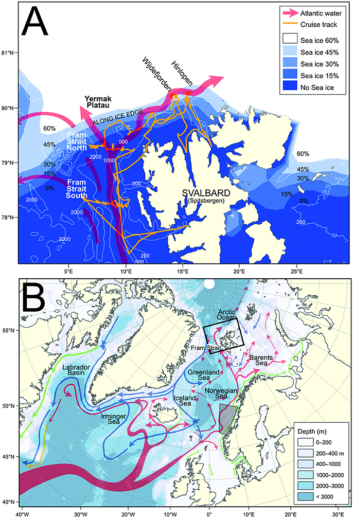
Figure 1. (A) Details of Fram Strait and Svalbard archipelago including bathymetry, main Atlantic currents, average sea ice concentration during the survey and cruise track with names of transects. (B) Bathymetric map of the Northern Atlantic with major currents superimposed. Hatched region refers to area covered by transects t1–t9 of Melle et al. (1993).

The Arctic Ocean and adjacent seas are currently in a state of significant change due to atmospheric and ocean warming, considerable sea ice retreat, varying import and export of liquid freshwater, changes in ice thickness, and melt dynamics (see Comiso, 2003; Kwok and Rothrock, 2009; Rabe et al., 2011, 2014a; Wassmann and Reigstad, 2011; Polyakov et al., 2012; Onarheim et al., 2014; Haine et al., 2015). These factors impact physical characteristics such as stratification (e.g., Korhonen et al., 2013) and nutrient supply and may also affect timing of phytoplankton and ice algae blooms (e.g., Fernández-Méndez et al., 2015). Wassmann and Reigstad (2011) using an alternative scenario approach, elaborated on how these potential changes might impact the future Arctic ecosystem, focusing primarily on the timing, quantity, and quality of primary and secondary producers, but also range shifts, changes in abundance, growth, behavior, and community structure. Fossheim et al. (2015) document how demersal fish species in a boreal shelf community are expanding their distribution northwards in the adjacent Barents Sea as the Arctic is warming, and Haug et al. (2017) point to the fact that annual scientific ecosystem surveys in the northern areas, as well as the fisheries show indications of a recent northern expansion of several important commercial fish species including mackerel (Scomber scombrus), cod (Gadus morhua), haddock (Melanogrammus aeglefinus), and capelin (Mallotus villosus). The latter three stocks are now extending as far north as the shelf-break north of Svalbard.

Light is important for phytoplankton and ice algae growth, but also crucial for visually feeding predators and their potential prey. As ice retreats in the Arctic the light conditions are changing. With a warming ocean climate, it will be necessary to separate the role of the ambient light fields from that of temperatures for biogeographic boundaries of small fish and their plankton prey (Kaartvedt, 2008), as the light field is crucial for species interactions that influence community structure and have implications for biodiversity, food-web configuration, and trophic pathways. The importance of light during the mid-night sun period in summer in restricting high Arctic mesopelagic fish diel vertical migrations for safe foraging at shallow depths has also been emphasized (Kaartvedt, 2008). Such potential restrictions in the feeding excursion could also apply to other types of organisms that are normally associated with DSLs in the Norwegian Sea (Melle et al., 1993; Torgersen et al., 1997; Kaartvedt et al., 1998; Knutsen and Serigstad, 2001), the Irminger Sea (Magnússon, 1996; Sigurðsson et al., 2002; Anderson et al., 2005), and the Labrador Sea (Pepin, 2013; Fennell and Rose, 2015).

Many of the organisms constituting the Deep Scatter Layer (DSL) in the Northern Atlantic, and mesopelagic fish in particular (Pepin, 2013), depend on Calanus and similar types of prey abundant at overwintering depths. The copepods Calanus finmarchicus, Calanus glacialis, and Calanus hyperboreus, are key mesozooplankters in the investigated area. C. finmarchicus has its core habitat in the Norwegian, Irminger, and Labrador Seas; C. glacialis normally inhabits Arctic shelf seas, while C. hyperboreus has its main distribution area in the Greenland Sea, the Labrador Sea, and the Arctic Ocean (Conover, 1988; Hirche and Kwasniewski, 1997; Skjoldal, 2004; Arnkværn et al., 2005; Kosobokova and Hirche, 2009; Ji et al., 2012). These copepods provide an important connection between the primary producers and fish (Kaartvedt, 2008), although seabirds, whales, jellyfish, and other invertebrate predators can directly utilize these resources as well (Youngbluth and Båmstedt, 2001; Berge et al., 2012; Kwasniewski et al., 2012). The calanoids feed and reproduce during spring and summer months and have a prolonged overwintering phase in deep water (Berge et al., 2012).

Current knowledge of processes involving species interactions and behavior in the high Arctic is fragmentary. The classical paradigm of biological quiescence during the Arctic polar night, has been challenged by a series of works recently published concerning feeding hyperiid amphipods during Arctic-darkness (Kraft et al., 2013), mass-vertical zooplankton migration during Arctic winter driven by moonlight (Last et al., 2016), and unexpected levels of biological activity during the polar night (Berge et al., 2015). Berge et al. (2009) showed that diel vertical migration during the Arctic winter is an important feature of the zooplankton community, especially for copepods in the epipelagial. Continued warming of the Arctic is likely to result in more complex ecotones across the Arctic marine system (Berge et al., 2014).

Baseline information regarding physical, chemical, and biological conditions is lacking for many parts of the Arctic (Wassmann and Reigstad, 2011; Wassmann et al., 2011) and crucial information on processes, species interactions, and behaviorial patterns recently uncovered (Berge et al., 2009, 2014, 2015; Kraft et al., 2013; Last et al., 2016), suggests that current knowledge of the high Arctic marine ecosystem is incomplete. Thus, our understanding of the susceptibility of the Arctic ecosystem to a warmer ocean climate is limited and pathways along which changes will proceed are uncertain. Until recently it is the dynamics in the epipelagic zone, mostly focusing on fjord systems, that has been examined (Berge et al., 2009, 2014, 2015; Kraft et al., 2013; Last et al., 2016). These investigations provide, however, little insight on the deeper living mesopelagic community and the coupling between the epipelagic and the mesopelagic communities (cf. Pepin, 2013).

The focus region of this study is the Fram strait and north of Svalbard archipelago from the shelf waters into the deep adjacent basins. Although this region has been under change for some time, the deep-water biological (species composition and biomass) and physical properties are hypothesized to change at a slower rate than the surface waters. The objectives of this paper are to (1) describe the bioacoustic patterns and relate them to the distribution and abundance of plankton and fish caught by various types of gear throughout the water column, (2) to relate these findings to the processes that might contribute to the creation and maintenance of the observed patterns, (3) to compare the DSL found around Svalbard, with the DSL's observed in other regions of the Northern Atlantic, particularly along the Norwegian coast and to some observations from the western Atlantic Ocean, and (4) to propose techniques for monitoring further changes in the Arctic deep-water pelagic community.

Materials and Methods

This study is based on the SI_ARCTIC 2014 survey and was conducted with RV Helmer Hanssen from 19 August to 7 September 2014 (Figure 1). The cruise consisted of transects from the shelf to the deeper basins in the eastern Fram Strait, transects across the shelf from Northern Svalbard across the shelf break, and a section along the drift-ice north of Svalbard. This gave the opportunity to study changes across gradients in depth, sea ice/water masses and currents, as well as changes along the Atlantic current. For this study, we have used data from multiple gear types deployed to collect physical data and to sample zooplankton and fish as well as collecting multifrequency acoustics data along the ship's trackline.

Environmental Data

Temperature and salinity were measured using a Seabird 911plus CTD at all biological sampling locations, including some additional profiles at the continental slopes of transects (Ingvaldsen et al., 2016—see their Figure 1 for CTD station locations). The CTD was equipped with an oxygen sensor (SBE 43) and a Seapoint Chlorophyll Fluorometer and a rosette system for collecting water samples. The conductivity, temperature, depth, and oxygen sensors are serviced and calibrated once a year by the manufacturer (Seabird). In situ water samples for salinity calibration (conductivity sensor) were taken at every station at maximum depth. The resulting accuracies of the pressure, temperature, and salinity measurements are estimated to 0.3 dbar, 0.001, and 0.002°C, respectively. Water samples for Winkler titration of oxygen were not obtained during the current investigations. However, the CTD's SBE43 oxygen sensor was calibrated on 13 February 2013 and data from this sensor was used to obtain a crude evaluation of ambient oxygen levels during the investigation, but also PANGAEA data by Rabe et al. (2014b) for a partly overlapping area (9 CTD stations east of longitude 2°E), in the eastern area of the Fram Strait in late June 2014, have been examined for comparison. The oxygen data of Rabe et al. (2014b) given in μmol/l were converted to ml/l using the ICES Unit conversion tools (http://www.ices.dk/marine-data/tools/Pages/Unit-conversions.aspx) (accessed 11 June 2017), and the relationship: 1 μmol O₂ = 0.022391 ml. As a proxy for phytoplankton biomass we use chlorophyll estimates based on old Seapoint factory calibrated fluorescence data. These should be considered relative values (“μg·l⁻¹, uncalibrated”) comparable between stations and does not imply an absolute measure of phytoplankton biomass (see also “Environmental Setting”).

Current velocities were measured with a RDI Sentinel 300 kHz lowered acoustic Doppler profiler (LADCP) mounted on the CTD carousel. The LADCP data were processed using methods common in the oceanographic community (LDEO-IX-8, Visbeck, 2002) and the barotropic tidal components were removed using the Arctic Ocean Tidal Inverse Model (AOTIM-5, Padman and Erofeeva, 2004). Sea ice concentration for the survey period was obtained from the National Snow and Ice Data Center (NSIDC) (Cavalieri et al., 1996, 1999).

In the current work we present the environmental situation from one transect on the west side of Spitsbergen (Transect 2—Fram Strait North), actually quite similar to the transect further south (Transect 6—Fram Strait South), and one transect north of Svalbard (Transect 4—Hinlopen). These two transects (cf. Figure 2) represent reasonably well the physical oceanography of key areas in the region during the investigations.

FIGURE 2

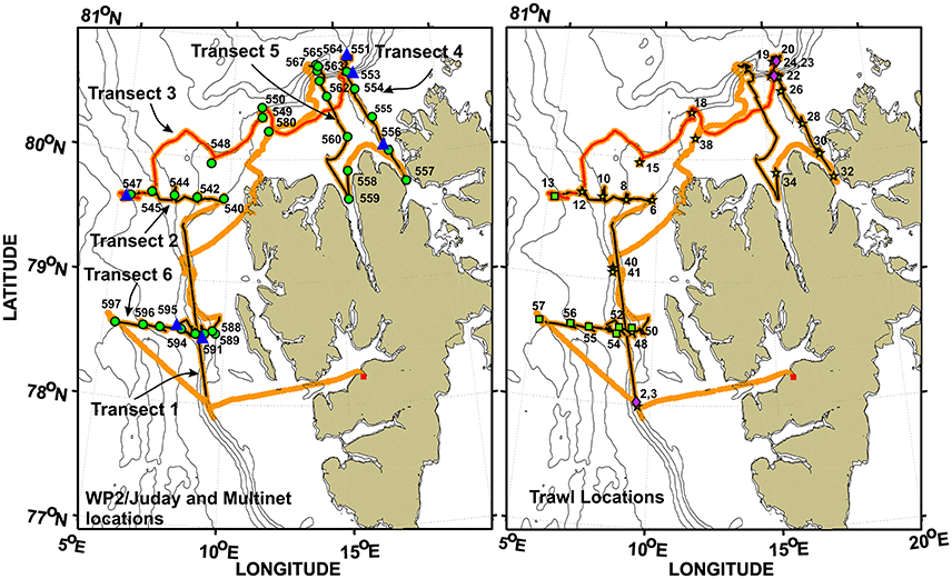
Figure 2. The RV Helmer Hanssen cruise track in orange with the sections of the track where the 38 kHz acoustic data were analyzed plotted in black, except for the Along Ice Edge transect that is red because it partly overlaps with the Fram Strait North and Hinlopen transects. Left: Station numbers and locations of the WP2/Juday net (green filled circles) and Multinet tows (blue triangles). Right: Station numbers and locations where the mid-water trawls were taken (cf. Tables 5, 6). Harstad trawls are designated by stars, Macroplankton trawls by diamonds, and Åkra trawls by squares. Transect 1, Along Shelf Break; Transect 2, Fram Strait North; Transect 3, Along Ice Edge; Transect 4, Hinlopen; Transect 5, Wijdefjorden; Transect 6, Fram Strait South.

Acoustic Data Collection

Acoustic data for estimation of the distribution and abundance of water column plankton and fish were collected with calibrated EK60 echo sounder split beam systems at the acoustic frequencies 18, 38, and 120 kHz at 1 ms pulse duration. The echo sounders were connected to transducers mounted on a protruding instrument keel with transducer faces ~3 m below the hull, usually ~8.5 m below the sea surface. The lower working threshold in terms of volume backscattering strength (S_v) in dB was set to −82 dB re 1 m⁻¹ (MacLennan et al., 2002). The vessel's EK60 systems are normally calibrated in January every year using standard methods and spheres (Foote et al., 1987; ICES, 2015a) and are known to be very stable over time (Knudsen, 2009). For the period 2010–2016 the vessel's 38 kHz EK60 system showed a <0.1 dB variation in S_v transducer gain.

Multi-frequency scrutinizing and target strength analysis were conducted with the Large Scale Survey System (LSSS) post processing system as described by Korneliussen et al. (2006, 2016), which also was used for exporting files for subsequent analysis by Matlab, Excel, or Systat. The processing involved selection of data to exclude and include, manual removal of noise (acoustic, electric, bubble, temporal noise from e.g., trawl sensors during trawl operations), correction of erroneous bottom detections, and surface originated noise. The allocation of Nautical Area Scattering Coefficient [NASC, s_A (m² nmi⁻²), MacLennan et al., 2002] values to various species or species groups and storage of these values in the database was done for 38 kHz frequency. In the upper ~200 m, where the signal/noise ratio on the 120 kHz echo sounder is above acceptable levels, all three frequencies were taken into account when inspecting the frequency response while below this depth, only 18 and 38 kHz were considered. Sequential thresholding was used to differentiate strong scatterers from weak scatterers. In the process the lower threshold (S_v) (LSSS–color scale, Korneliussen et al., 2016), was moved from the standard −82 dB upwards to a value where only the strongest scatterers remain visible on the echogram (e.g., −60 dB). The s_A corresponding to this S_v threshold was then allotted to the species or species group normally known to have a Target Strength (TS) above this threshold. Subsequently this s_A was subtracted from the total, and the remainder allotted to weak scatterers with TS below this threshold. In the Supplementary Material additional details are presented on the use of “sequential thresholding” and relative frequency response defined according to Korneliussen and Ona (2003) as r(f) ≡ s_v(f)/s_v (38 kHz), where s_v is the volume-backscattering coefficient, and the response at the acoustic frequency f is normalized to that at 38 kHz. Trawl data were used to corroborate the interpretation of the acoustic data. The acoustic backscattering data in the reports were in the form of s_A for 10-m depth intervals in units of (m² nmi⁻²).

The fairly low noise level enabled measurements down to about 800 m, while the main DSL concentrations were found not deeper than 600 m. Total backscatter was allotted using LSSS to the stronger scattering target categories (SC) 0-group fish, cod, capelin, redfish, and others (see ICES, 2015b; Korneliussen et al., 2016), then lumped to the category Strong_SC. The remaining backscatter including the micronekton krill, amphipods, and mesopelagic fish were lumped into the category Weak_SC. The two categories were summed to provide a third, “Total backscattering.” Micronekton as used herein is a combination of fish, krill, and a number of other animals in the 1–20 cm size range, nearly overlapping in size with what we normally term macroplankton (Cartes, 2009).

The above acoustic data for the three final categories were transformed to S_A [Nautical area scattering strength dB re 1 (m² nmi⁻²) by S_A = 10 log10 (s_A) and visualized on five of six transects along the ship's cruise trackline (Figure 2, Table 1) using “EasyKrig_V3.0.1-Matlab2012a,” a Matlab based tool written by Chu (2004, ftp://globec.whoi.edu/pub/software/kriging/easy_krig/; accessed 15 July 2013). The variogram model was the “general exponential-Bessel” and the Ordinary Kriging model was Point to Point with nugget set to 0, sill <1, length around 0.5, power > 1.5, and range ~0.5.

TABLE 1

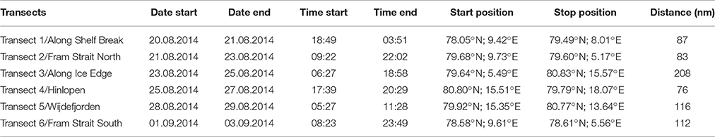
Table 1. Logistics information for acoustic Transects 1–6.

The scrutinized 38 kHz acoustic data were integrated vertically to provide the pattern of horizontal variability along each transect. Data were also averaged horizontally to provide vertical profiles of backscattering for particular subsections along each transect (Table 2). These subsections represent part of transects that were reasonable homogeneous with respect to bathymetry and acoustic backscatter in the DSL over the distance of the subsection, facilitating comparison of these between transects. In addition, acoustic data for selected subsections of transects were integrated to highlight the horizontal variability amongst the Weak_SC and Strong_SC categories along the transects. To compare the DSL in the different areas, the weighted mean depth of the backscattering (WMD) in the depth intervals of 250–600 m for each acoustic sub-section was computed using the following equation:

$\begin{array}{l}WMD={\displaystyle \sum _{j=1}^N}{z}_j{s}_{A_j}/{\displaystyle \sum _{j=1}^N}{s}_{A_j}\end{array}$

where z is the depth of interval j, s_A is the nautical area scattering coefficient value for that depth interval, and N is the number of depth intervals. The first transect along the shelf slope edge (Table 1), was not included in these analyses because of the variable bottom depth along the cruise track and the lack of ground-truth tows. All description of the patterns on transects and subsections are based on the 38 kHz data.

TABLE 2

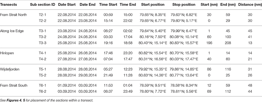
Table 2. Logistics information for acoustic subsections within Transect 2 to Transect 6 (T2–T6).

Biological Data Collection

Samples of fish, micronekton, and zooplankton were collected with a variety of net and trawl systems (Figure 2). These included the Harstad trawl (Nedreaas and Smedstad, 1987; Godø et al., 1993; Dingsør, 2005), having a circumference of 320 m (Terje Hemnes, pers. comm., Åkrehamn Trålbøteri AS, http://www.tral.no/), although dimensions slightly change when being towed (Underwood et al., 2014), the Macroplankton trawl having a fixed mesh size of 4 × 4 mm from the mouth of the trawl to the cod-end, an approximately rectangular mouth opening of ~38 m² and a 92 m circumference (Melle et al., 2006; Wenneck et al., 2008; Krafft et al., 2010; Heino et al., 2011), the Åkra trawl (Valdemarsen and Misund, 1995), the current version with a trawl circumference of 538 m, the MIK-Ring Net (Munk, 1993; ICES, 2013—3.14 m²/1600 μm mesh size), the Multinet (Weikert and John, 1981—0.25 m²/180 μm mesh size), and the WP2 (0.25 m²)/Juday (0.1 m²) net (Juday, 1916; Working Party 2, 1968; both nets 180 μm mesh size). Trawl speed was ~2.5–3.5 knots, slightly depending on trawl being used and depth of trawling was monitored using a Scanmar depth sensor and trawl sonde. The Macrozooplankton trawl was additionally equipped with a combined Scanmar speed/symmetry sensor to allow the trawl speed through the water to be measured thereby allowing computation of the water volume filtered by the trawl.

The principal zooplankton sampling system was the combined WP2 and Juday net pair mounted on a single frame with two rings on which the net mouths were tied. This system was operated vertically, usually to within 10 m of the bottom, at most stations where the CTD was deployed. The WP2 sample was split and 50% was fixed in borax-buffered 4% formaldehyde for identification and enumeration purposes, while the other 50% was used for biomass estimation. This part was divided into three size fractions using sieves with mesh-sizes 2,000, 1,000, and 180 μm. Most animals retained on the 2,000 μm sieve were sorted, identified, and counted (Chaetognaths, the copepods Paraeuchaeta sp. and C. hyperboreus), while individual lengths of amphipods, fish, krill, and shrimps, were additionally measured after taxonomic identification and prior to rinsing in fresh water. The biomass retained on the 1,000 and 180 μm sieves as well as the identified animals belonging to the aforementioned groups above retained on the 2,000 μm sieve, were put on pre-weighed aluminum dishes and dried in an oven at 60°C overnight, after which they were packed and stored in a freezer at −20° awaiting new drying and weighing at the IMR onshore laboratory. After drying the summed dry biomass per group was measured.

The trawls were used to obtain a qualitative and semi-quantitative understanding of larger micronekton and fish that were present in the acoustic scattering structures observed. Hauls either targeted specific scattering structures (“targeted hauls”) with the aim to identify their constituents (Åkra and Harstad trawls) or they were standardized hauls to enable documentation of important acoustic scatterers in the water column. These included oblique hauls from near the bottom to surface using the Macroplankton trawl both in shallow and deep waters and standardized step-wise 0-group hauls (Dingsør, 2005), conducted in the uppermost 0–20–40 m using the Harstad trawl. With a trawl vertical opening of ~20 m, the sampling range was 0–60 m. For the Åkra trawl and Harstad trawl catches total numbers and wet weight were obtained for each taxonomic group or species being determined. Lengths were recorded for all specimens in the catch, and weight, age (by otoliths), maturity stage, and stomach content were determined for a subsample of the fish catch, while another subsample of the invertebrate part of the catch was worked up to species or genus if possible or to coarser groups like “Amphipoda” or “Euphausiacea” and their numbers and weights determined (±0.1 g). The Macroplankton trawl catches were worked up in a similar way after first determining total wet weight of catch (kg). Normally, all larger fish and jellyfish were determined to nearest possible taxon, counted, and wet weight measured. Because of the scarcity of fish in theses catches, individual lengths and wet weights were normally obtained. The remaining invertebrate catch was subsampled and worked up to nearest possible taxon and their numbers and wet weight determined (±0.1 g). In addition, individual lengths of amphipods, krill, and shrimps were measured (fresh length ± 1 mm). Due to methodological issues, such as depth of trawling, trawl variable mesh size, and differences in trawl mouth opening and mesh size between trawls, catches from the Harstad and Åkra trawl hauls were standardized to kg nmi⁻¹. The Macroplankton trawl catches were standardized to g m⁻³ using a computed haul volume filtered. The tabled numbers of Harstad and Åkra trawl species abundances must be considered indicative of their presence rather than actual abundances.

The Institute of Marine Research (IMR) fully adheres to Norwegian laws relevant to Ethics in Science as well as Animal Welfare. The legal and institutional framework within which IMR operate is detailed in OECD (2012, Part III, Chapter 21, p. 373–398). Under the current legal framework, there is no special permit requirements for at sea research and monitoring activities which do not involve experiments with live animals.

Results

Environmental Setting

Atlantic Water (temperature >0°C and salinity >34.9, derived from Rudels et al., 2005) dominated from 1,000 m depth up to the surface layer in the Fram Strait North transect (Figures 3a,b). Over-riding the Atlantic Water was a fresher surface layer along most of the transect, although with strong lateral gradients (Figure 3a). In the western part of the transect, the presence of sea ice and melt water (with temperature below 0°C and low salinity) created a pronounced surface layer in the upper 30–40 m. Associated with this melt water layer was low fluorescence-chlorophyll values in the upper 20 m and a sub-surface maximum fluorescence-chlorophyll around 40 m, between the Atlantic Water and melt water. On the eastern side of the transect, the fluorescence-chlorophyll values indicated rather evenly distributed phytoplankton in the top 30 m.

FIGURE 3

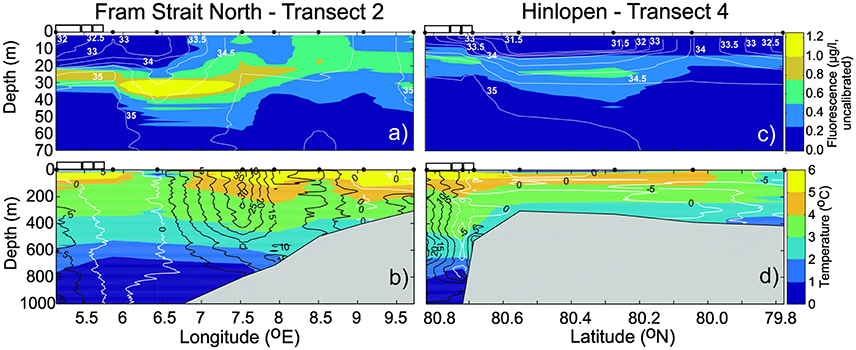
Figure 3. Upper panels show fluorescence (colors) and salinity (lines) in the upper 70 m in section Fram Strait North (a) and Hinlopen (c). Lower panels show temperature (colors) and across section velocity (lines, in cm s⁻¹) in the upper 1,000 m in section Fram Strait North (b) and Hinlopen (d). The white rectangles on top of the plots to the left indicate presence of sea ice. Black filled circles on top of each panel indicate position of CTD stations.

Despite rather weak horizontal temperature gradients in the Atlantic Water, there were strong gradients in velocity (Figure 3b). While the middle of this transect was dominated by strong northward Atlantic Water flow (reaching velocities of 30 cm s⁻¹), both the eastern and western sides showed rather weak flow.

North of Svalbard, at Hinlopen, the northern most part of the transect was dominated by eastward flow of Atlantic Water between 10 and 1,000 m depth (Figures 3c,d). On top of this (in the upper ~10 m) melting sea ice made a fresh, cold surface layer. As opposed to the Fram Strait north, the subsurface chlorophyll maxima under the ice and along transect was much less prominent and did not reach the uppermost 10 m of the water column (Figure 3c). A westward current was evident at the shelf break. Crossing the shelf break onto the shelf, the currents were low and Atlantic Water dominated in most of the water column, except for the innermost (southernmost) part of Hinlopen. Phytoplankton fluorescence was higher on the outer shelf and beyond, than in the innermost parts.

The water column at all stations and to depths of ~2,600 m, seemed very well oxygenated with values in the range ~5.3–7.6 ml l⁻¹, while measurements >300 m were in the range 5.34–5.74 ml l⁻¹ with an average of 5.57 ml l⁻¹ (N = 5,408) based on the Helmer Hanssen Seabird SBE43 oxygen sensor data. However, the PANGAEA data calibrated and corrected using Winkler titration (Rabe et al., 2014b), from the same year and region (cf. section Materials and Methods), show that the oxygen values at depths greater than 300 m, were clearly higher than our values, within the range 6.78–7.28 ml l⁻¹ and with an average of 6.98 ml l⁻¹ (N = 18,665). Thus, the Rabe et al. (2014b), average value for all measurements below 300 m was 1.4 ml l⁻¹ higher than the average value based on our own measurements.

Bioacoustics Patterns

The vertically integrated water column backscattering, s_A, was highest along the western Svalbard shelf break (Transect 1) and across the southern portion of the Fram Strait (Transect 6—Table 3). The Strong_SC backscattering dominated over the Weak_SC except across the northern Svalbard shelf and into the Arctic Ocean (Transects 4 and 5), and only on the Hinlopen section (Transect 4) was the Weak_SC greater than the Strong_SC because there were few strong scatterers (Table 3).

TABLE 3

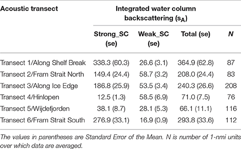
Table 3. Average water column integrated s_A, Nautical area scattering coefficient in units of (m² nmi⁻²) at 38 kHz for categories Strong_SC, Weak_SC and Total on acoustic transects 1–6 as shown in Figure 2.

For the Fram Strait South transect (Figure 2) a significant feature was the high backscattering at the surface (Figure 4). It extended from the coast and was most intense at the midway point and dominated by the Strong_SC category (Figure 5) that can also be seen from the total integrated values and for depths <100 m (Figure 6). The very strong backscattering in the upper 100 m (Strong_SC) resulted in the total backscattering for the water column being dominated by this component over the entire transect (Figures 6, 7 and Tables 3, 4). The Strong_SC contribution to the deep-scattering layer from 300 to 450 m was more important than the Weak_SC until midway along the transect to the west. Then the Strong_SC fraction declined and in the western portion of the subsection the Weak_SC accounted for the majority of the backscatter below 100 m depth (Figure 6).

FIGURE 4

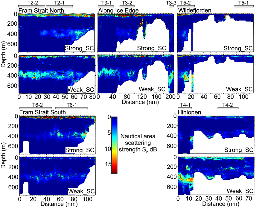
Figure 4. Distribution of the strong backscatter category (Strong_SC, Upper) and the weak backscatter category (Weak_SC, Lower) for the transects, Fram Strait South (T6), Fram Strait North (T2), Along Ice Edge (T3), Wijdefjorden (T5), and Hinlopen (T4). Values are the Nautical area scattering strength, S_A = 10*Log10 (s_A), dB re 1(m² nmi⁻²). Gray rectangles above transects indicate position of subsections. x-axes are of unequal length.

FIGURE 5

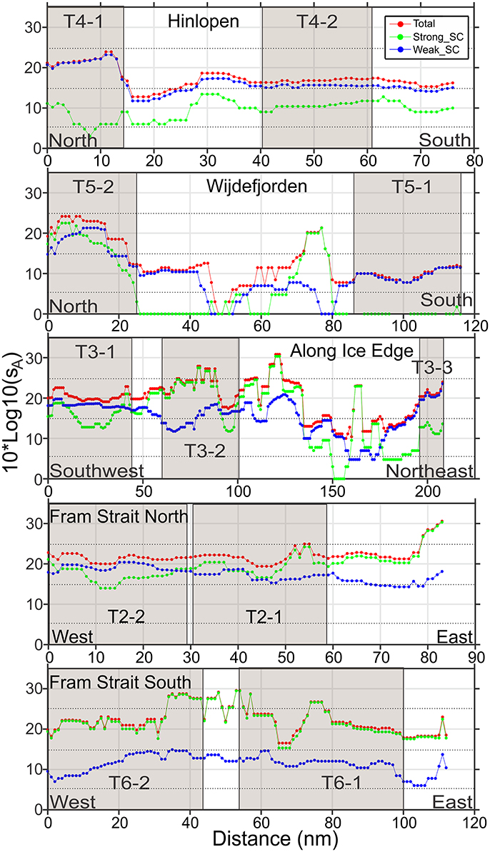
Figure 5. Vertically integrated s_A, Nautical area scattering coefficient in units of (m² nmi⁻²) presented as Nautical area scattering strength, S_A = 10*Log10 (s_A), dB re 1(m² nmi⁻²) along transects, arranged from south-west (lower) to north-east (upper): T6, Fram Strait South; T2, Fram Strait North; T3, Along Ice Edge; T5, Wijdefjorden; T4, Hinlopen. Beige boxes indicate position of subsections. x-axes are of unequal length.

FIGURE 6

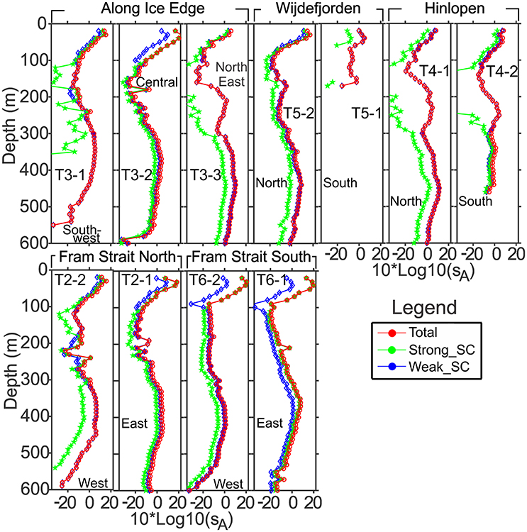
Figure 6. Subsection averaged vertical profiles of acoustic backscattering s_A, Nautical area scattering coefficient in units of (m² nmi⁻²) for the categories Weak_SC, Strong_SC and Total s_A, presented as Nautical area scattering strength, S_A = 10*Log10 (s_A), dB re 1(m² nmi⁻²). T2, Fram Strait North; T3, Along Ice Edge; T4, Hinlopen; T5, Wijdefjorden; T6, Fram Strait South.

FIGURE 7

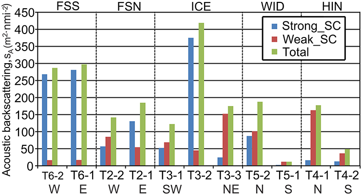
Figure 7. Integrated water column acoustic backscattering s_A, Nautical area scattering coefficient in units of (m² nmi⁻²) for the categories Weak_SC, Strong_SC and Total s_A by subsection within transects as indicated in Figure 5. W, West; E, East; S, South; N, North; NE, North-east; SW, South-west; FSS, Fram Strait South; FSN, Fram Strait North; ICE, Along Ice Edge; WID, Wijdefjorden; HIN, Hinlopen.

TABLE 4

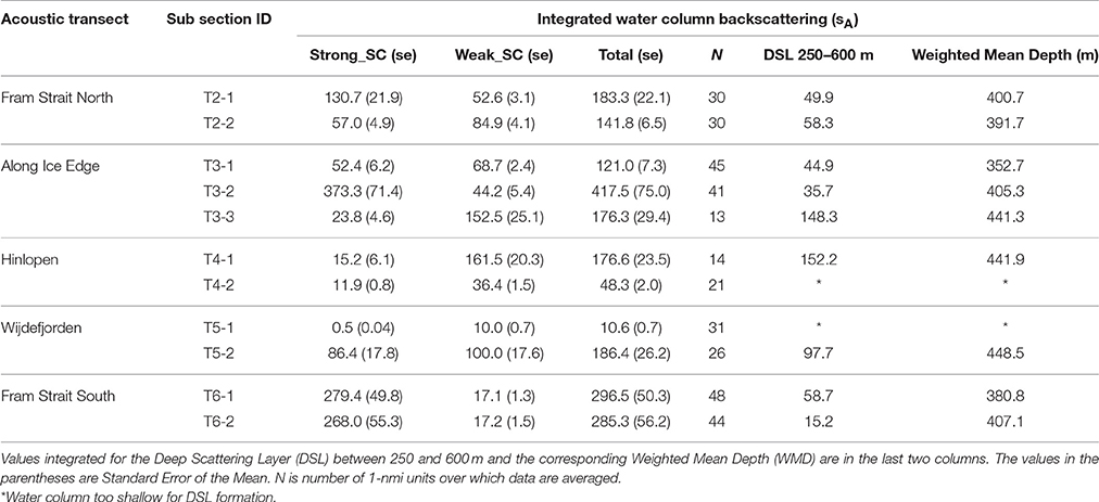
Table 4. Average water column integrated s_A, Nautical area scattering coefficient in units of (m² nmi⁻²) at 38 kHz for subsections and categories Strong_SC, Weak_SC and Total s_A on acoustic Transect 2 to Transect 6 (T2–T6).

Along the Fram Strait North transect (Figures 4, 5), high backscattering at the surface, also seen in the Fram Strait South transect, was evident, with a major contribution from the Strong_SC fraction, but there were scattered patches of high scattering in the Weak_SC fraction as well. A moderately strong scattering layer extended from the continental slope to the western end of the transect between 300 and 450 m. An important feature was that the DSL Strong_SC fraction was present from the continental slope to about two-thirds of the distance to the west and then became insignificant; the DSL Weak_SC contribution was moderate from the continental slope to the point where the Strong_SC scattering lost significance and then became stronger to the western end of the transect (Figures 4, 5). The abrupt change in the contributions of these two fractions occurred about where there was a cross-over from warm Atlantic water (>6°C; salinity >34.9) to colder melt water (~0.5–2.5°C; salinity ~31.8–33.0) at the sea surface (Figure 3). For the easternmost subsection (T2-1) closest to the continental shelf, Strong_SC backscattering was higher than Weak_SC in the upper 100 m (Figure 6) while the Weak_SC backscattering was higher than the Strong_SC below 100 m. Still the Strong_SC component was dominant in the water column as a whole (Figure 6, Table 4). Further offshore on Fram Strait North (T2-2), Strong_SC backscattering was lower and Weak_SC backscattering was higher throughout most of the water column (Figures 6, 7, Table 4). The pattern observed is nearly identical to the pattern seen for the Fram Strait South.

On the Along-Ice-Edge transect, from the western end of Fram Strait North to the northernmost station close to the start of the Hinlopen transect (Figure 2), the acoustic backscattering paralleled that observed on the Fram Strait transects. There was strong surface to 50 m backscattering until reaching about 140 nmi along the section. For the south-western subsection (T3-1) it was the Weak_SC that dominated the backscattering through most of the water column (Figure 6), including the DSL between 300 and 450 m. For the central deep shelf area subsection (T3-2, Figures 5–7), the Strong_SC component dominated in terms of total integrated backscatter, largely due to that component dominating in the uppermost 100 m of the water column. The variable backscattering further east (Figures 4, 5) is due to Strong_SC scattering that increased to moderate levels when the bottom shoaled to about 250 m (~nautical mile 110). Very low backscattering occurred at the shallowest portion of the transect (about 100 m) at nm 170. In the far northeast area (T3-3), there was again a DSL from 300 to 500 m dominated by high Weak_SC scattering.

The Hinlopen and Wijdefjorden transects across the Northern Svalbard Shelf region and into the deep Arctic slope water had quite similar backscattering patterns (Figure 4). The northern part of the Hinlopen transect had water depths up to 1,850 m, but due to a steep slope and lower quality acoustic data acquired during off-shelf station work, useful acoustic data were recorded to around 700 m bottom depth off the shelf and ended in Hinlopen Strait. Total backscattering was dominated by Weak_SC for the whole transect (Figure 5, Tables 3, 4), and is also reflected in the subsection vertical profiles (T4-1, Figures 5–7, Table 4). In this area, the marine mammal observers noted the presence of a number of whales. On the shelf, water column scattering was moderate and mostly in the upper 50 m with scattered patches of moderate to high Weak_SC backscattering also occurring in the 200–350 m depth zone (T4-2).

The more western Wijdefjorden transect was mostly over very shallow shelf waters. Moderate surface to 50-m backscattering was evident over the shelf and most due to the Weak_SC fraction (Tables 3, 4). Midway along the shelf, near a shallow bottom feature, there was strong scattering by the Strong_SC fraction (Figure 5). To the north beyond the shelf break (Figure 2), there was again strong surface scattering in which both Strong_SC and Weak_SC contributed significantly (T5-2, Figures 5–7) and as in the previous transects, there was strong backscattering centered around 400 m that was dominated by the Weak_SC fraction below 100 m depth (Figure 6).

The Weighted Mean Depth of the DSL backscattering values between 250 and 600 m for all transects averaged 407 m (Table 4). The three deepest WMD values (all > 440 m) were in the Arctic Basin: the Along Ice Edge transect (T3-3), Wijdefjorden (T5-2), and Hinlopen (T4-1). The shallowest (352 m) was in the first subsection (T3-1) along the Ice Edge transect. The integrated DSL values were mostly <50% of the total 600 m water column s_A except in the Arctic Basin where the DSL was about 80% of the total 600 m water column s_A (Table 4).

Biological Distributions

Mesozooplankton Sampling with WP2 Net

Mesozooplankton biomass collected with the WP2 net (Figure 2) was occasionally very high and at a couple of stations on the west side of Svalbard up to about 63.5 g m⁻² (Figure 8). The size fractionated mesozooplankton biomass displayed both north-south and east-west gradients in the study region. The Fram Strait South transect had an overall average biomass of 33.9 g m⁻². Individual stations at the slope deeper than about 500 m had the highest values, all above 30 g m⁻² except for station 596 where only half the water column was sampled (Figure 2). Most of the central stations located in the slope region were dominated by the smallest (>180 μm) size fraction. The Fram Strait North transect had similar features and had an overall average biomass of ~30 g m⁻². The stations located near the ice edge and undertaken while moving north-east toward the easternmost part of the Hinlopen transect had a substantially lower average biomass of 13.9 g m⁻². For the three ice edge stations, the size fractions >180 μm and 1,000–2,000 μm had most of the biomass recorded. The Wijdefjorden transect showed an overall average biomass of 11.7 gm⁻², but this transect was dominated by stations located on a shallower portion of the northern Svalbard shelf, and only the two northernmost stations with bottom depths exceeding 500 m had biomass values above 16 g m⁻². In this area, the two smallest size fractions dominated the biomass, with the 180 μm size fraction often having the highest biomass (Figure 8).

FIGURE 8

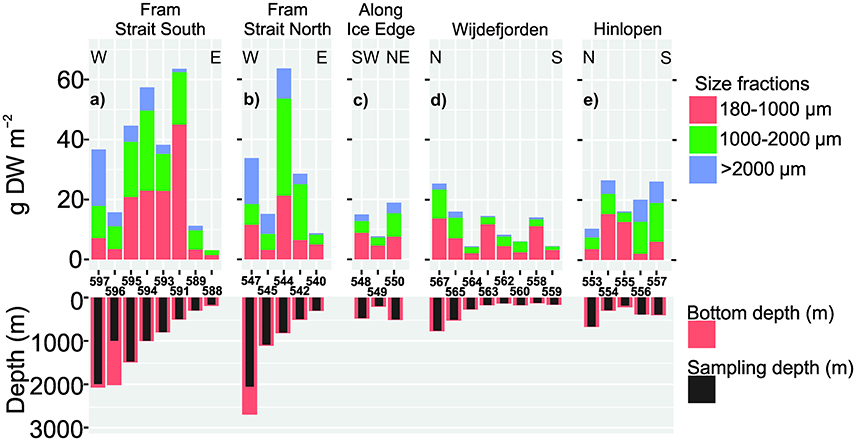
Figure 8. Upper: Regional size-fractionated mesozooplankton biomass in g DW m⁻² from a vertically operated WP2 net (180 μm mesh size). Lower: Bottom and sampling depths along transects. Station numbers between panels. W, E, N, S, SW, NE represent West, East, North, South, South-West and North-East respectively. (a) Fram Strait South (T6), (b) Fram Strait North (T2), (c) Along Ice Edge (T3), (d) Wijdefjorden (T5), and (e) Hinlopen (T4).

On the easternmost Hinlopen transect with deeper shelf depths, the overall average biomass was 19.9 g m⁻², nearly twice the average for the Wijdefjorden transect (Figure 8). Although the two smallest size fractions dominated on all stations along the transect, the largest size fraction was more important and similar to some samples on the Fram Strait transects (Figure 8).

Macroplankton and Fish Sampling with Trawls

On the Fram Strait South transect several catches taken in the DSL with the large pelagic Åkra trawl showed that larger cod were present in moderate numbers along with mesopelagic fish and krill (Table 5). Due to its large mesh size this trawl, however, does not effectively sample micronekton and they are underrepresented in the catches.

TABLE 5

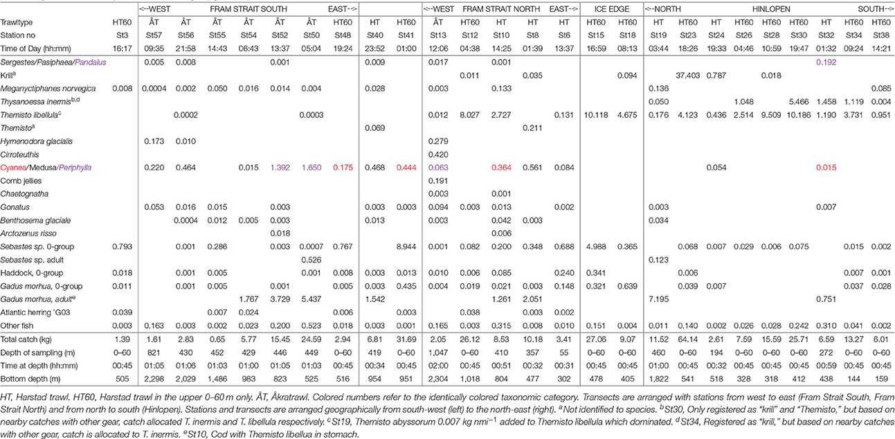
Table 5. Taxonomic composition in wet weight (kg nmi⁻¹) for Harstad- and Åkratrawl catches.

Along the Fram Strait North transect, shelf catches from the Harstad trawl in the upper layer (0–60 m) had a high abundance of Sebastes sp. 0-group fish that dominated the biomass and were the main constituent of the Strong_SC acoustic backscattering (Table 5). Typically, larger fish like cod and Greenland halibut were found at the shelf break/slope region and beyond. On one occasion, St10 (Figure 2), the cod had apparently been feeding on the Arctic hyperiid Themisto libellula. Westward on this transect, 0-group fish were still present in upper 60 m, but were less abundant. Themisto libellula was observed in very high abundance in a shallow haul (0–60 m) at St12 with a bottom depth of around 1,000 m (Table 5). This species was often observed in near surface layers and was a key contributor on many stations to the acoustic Weak_SC category. We also observed that trawls lowered into the 300–500 m depth range or deeper, sampled organisms that are regular or temporary constituents of the DSL. These include the mesopelagic fish Benthosema glaciale, the krill Meganyctiphanes norvegica, the deep-water shrimps Sergestes arcticus/Pasiphaea sp. complex, and Hymenodora glacialis, the octopod Cirroteuthis sp., and the crown jellyfish Periphylla periphylla.

On the northern Svalbard shelf along the Hinlopen transect, the key components in the trawl catches were krill and amphipods (Table 5). Particularly high weights were found in hauls from the upper 0–60 m. The Weak_SC acoustic backscattering that dominated in this area was largely due to these two components. The krill species M. norvegica, Thysanoessa inermis, and Thysanoessa longicaudata were all present in these trawl catches, but M. norvegica was more abundant toward the northern part of the shelf and in the Arctic slope region. The amount of fish along the Hinlopen transect was substantially lower than the abundance of krill and amphipods in terms of weight nmi⁻¹ trawled. The 0-group fish (e.g., Sebastes sp.) were far less abundant north of Svalbard than further west and south (Table 5).

Macroplankton trawl hauls (Figure 2) were taken on the deep slope bordering Sofiadypet (the deep Arctic Ocean Area north of Svalbard) to 1,100 and to 408 m depth (St20,22-Table 6). The deep haul included the DSL and the main contributors to the biomass caught, in decreasing order were; T. inermis, Chaetognatha, the hydrozoan jellyfish Aglantha, the mesopelagic shrimp H. glacialis, M. norvegica, and T. libellula. Regular representatives of the mesopelagic community were Chaetognatha, Aglantha, and H. glacialis. The mesopelagic fish B. glaciale was observed in moderate biomass and the white barracudina Arctozenus risso was present. Slightly further south at deep shelf location St22, the Macroplankton trawl to 408 m also caught B. glaciale and the abundance of the euphausiids M. norvegica and T. inermis was two times higher than further off the shelf (Table 6). Combined with the other trawl observations (Table 5), these data support the Weak_SC as a very important acoustic component across the central shelf and the slope region north of Svalbard.

TABLE 6

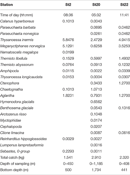
Table 6. Macroplankton trawl wet weight catch composition (g 1,000 m⁻³).

Discussion

Although acoustics are regularly used to map the distribution of pelagic fish both in the Norwegian and Barents Seas (Toresen et al., 1998; Michalsen et al., 2013), there are only a restricted number of studies around the northern Atlantic where acoustic techniques have been applied in open ocean regions to examine large-scale acoustic backscattering structures (Melle et al., 1993; Kaartvedt et al., 1996, 1998; Magnússon, 1996; Torgersen et al., 1997; Dale et al., 1999; Knutsen and Serigstad, 2001; Anderson et al., 2005; Pepin, 2013; Norheim et al., 2016; Siegelman-Charbit and Planque, 2016). Most studies have focused on the more accessible fjord populations of fish and plankton, addressing specific issues related to predator prey interactions and diel vertical migration (Falk-Petersen et al., 2004; Kaartvedt et al., 2008; Berge et al., 2009, 2014; Dypvik et al., 2012).

The current study is to our knowledge one of very few that incorporates biological and acoustic data from a larger part of the epipelagic and the mesopelagic zone (200–1,000 m depth), in the Northern North Atlantic on the boundary to the Arctic Ocean. This is a region where little comparative information is available, particularly for the deeper part of the water column.

Resonance

Irigoien et al. (2014) estimated the mesopelagic backscatter from depths of 200–1,000 m across the world's major ocean basins between 40°N and 40°S to have an average s_A of 1,864 ± 1,341 s.d. (m² nmi⁻²), while individual estimates ranged from 158 to 7,617 m² nmi⁻² at 38 kHz. They concluded that swimbladder “resonance” (the considerable amplification of backscattering that occurs when an object is insonified at a frequency that matches its own natural frequencies of vibration) was not a significant issue in most areas that were covered, which is interesting as a range of ecosystems and certainly quite diverse ensembles of mesopelagic species must have caused the backscattering recorded. Probably most of these communities were far more diverse in terms of number of species and types of swimbladder morphology than the simple mesopelagic community of the northeastern North Atlantic encountered during the current study. Swimbladder “resonance” is a well-known concern in the history of mesopelagic and myctophid acoustics (Sætersdal et al., 1999; Godø et al., 2009; Irigoien et al., 2014; Davison et al., 2015). It can complicate interpretation of s_A-values in time and space, and may result in overestimation of species abundance and/or biomass (see Sætersdal et al., 1999).

What could be interpreted as resonance during the current investigations was observed in the surface waters and most likely produced by 0-group fish as no mesopelagic fish where caught in the 0-60 m hauls at any time of the day (Table 5). The species that dominated our catches at depth (Table 5) and could be responsible for resonance, like B. glaciale, has a swimbladder either partly filled with gas and oil or no gas at all, and also less gas with increasing size (Bardarson, 2014; Scoulding et al., 2015). Modeled estimates based on a swimbladder volume of 1.16 mm³ in a 4.6 cm long B. glaciale gives resonance slightly above 18 kHz at 100 m depth while at 300 m the same sized swimbladder will give resonance slightly below 38 kHz (Bardarson, 2014). At 300 m there is a 15 dB difference in the target strength (TS₁₈ ≈ −75 dB, TS₃₈ ≈ −60 dB) for a B. glaciale of the above size (Bardarson, 2014). However, during the current study there was little evidence of resonance at depth as indicated by the frequency response at 18 kHz relative to 38 kHz, r(18 kHz), that was frequently close to 1.0 over a greater part of the investigated area (see Supplementary Material). Also, the White Barracudina (Arctozenus sp.) that were regularly caught at depth, does not have a swimbladder, implying that it would be a quite weak scatterer in the mesopelagic zone. Larger fish (i.e., cod and redfish) are known to have well developed gas filled swimbladders and a much higher Target Strength (TS) compared to the mesopelagic representatives above. They were, however, caught at depth, but seemed to be associated with the shelf and slope region, although occasionally their distribution was extended further off the continental shelf (Ingvaldsen et al., 2017).

Key Features along Acoustic Transects

The acoustic transects exhibit some key features (Figure 4). There was strong patchy scattering between the surface and about 50 m throughout most of the study area. In deep waters off the shelves there was strong scattering between 200 and 600 m dominated by larger fish (Strong_SC) close to the slope/shelf break and associated with the warm Atlantic Water moving north toward the Arctic Ocean. West of Svalbard the larger fish component diminished rapidly westwards, while the Weak_SC scatterers were increasingly dominant. There were no observed signals in temperature or salinity in the deeper portion of the water column that could be associated with the change in scattering structures across the deeper part of these western transects. However, the location of the Arctic front at the surface corresponded roughly to where the DSL changed from being dominated by larger fish to being dominated by Weak_SC at depth (Figures 4, 6). Also, in the western part of the transects, the Atlantic Water flow was weaker and sea ice and melt water dominated in the surface layer. In addition, west of the core Atlantic inflow along the Svalbard shelf there was almost no northwards flow (cf. Figure 3) over the entire water column. A similar pattern in acoustic backscattering at 38 kHz was observed by Dale et al. (1999) during an east-west transect from the Bear Island (74°30′N, 19°01′E) along latitudes 74 and 75°N to ~10°W in November 1995. The mesopelagic scatterers in the deeper part of the water column (>250 m) decreased substantially around 150 km west of Bjørnøya (~14°E) when approaching Arctic water masses.

In a 1993 survey of the Norwegian Sea (62–70°N) during June/July, the “deeper layer” (~200–500 m) DSL was 40% or more of the water column integrated backscatter and decreased in the total backscattering from south to north by approximately a factor of 2 (Figure 9; Melle et al., 1993). The integrated area backscattering coefficient (s_A–m² nmi⁻²), averaged over transects where bottom depth exceeded 509 m, ranged between 180 and 460 m² nmi⁻². Melle et al. (1993) found no clear-cut temporal change between April, May, and June/July in the DSL acoustic layers. On the Norwegian Sea slope (65°00′N, 04°50′E) in June 2000 in 844 m of water, Knutsen and Serigstad (2001) reported values for the DSL of 400–2,000 m² nmi⁻².

FIGURE 9

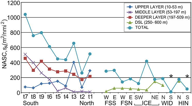
Figure 9. Left: Integrated Nautical area scattering coefficient (s_A) in units of (m² nmi⁻²) in layers 10–53, 53–197, and 197–509 m, averaged over individual transects t1–t9 in the eastern Norwegian Sea where bottom depth exceeded 509 m from ~62 to 68°33′N during the period June/July 1991, modified from Melle et al. (1993). Right: Integrated s_A for subsections of Fram Strait South (FSS), Fram Strait North (FSN), Along Ice Edge (ICE), Wijdefjorden (WID), and Hinlopen (HIN). W, E, N, S, SW, NE represent West, East, North, South, South-West and North-East, respectively. The central subsection along ice edge not explicitly marked. *Water column too shallow for DSL formation.

In the Irminger Sea, Magnússon (1996) observed a DSL between 400 and 800 m and latitudes ~60–68°N, although its vertical position varied somewhat depending on time of the year. Overall the integrated values over the water column ranged from 1,000 to 5,000 m² nmi⁻² and occasionally higher. In the same region, Anderson et al. (2005) showed integrated values for the 0–800 m water column during daytime in the same range (~600–2,000 m² nmi⁻²). The values of Magnússon (1996) and Anderson et al. (2005) are considerably above values for the region west and north of Svalbard and also generally higher than the average values for transects found in the south-eastern part of the Norwegian Sea around 62–64°N and 3–6°E (Melle et al., 1993; Knutsen and Serigstad, 2001). The Irminger Sea values are for the whole water column and are not entirely comparable to those of Melle et al. (1993). However, Anderson et al. (2005) reported daytime values in the 0–200 m layer that in most instances were <62 m² nmi⁻², while night-time values ranged from 42 to 235.8 m² nmi⁻², indicating that they are on the order of 10–100 times lower than the total water column (0–800 m) backscattering, thus emphasizing the importance and magnitude of the DSL itself.

The values recorded for the Irminger Sea (Magnússon, 1996; Sigurðsson et al., 2002; Anderson et al., 2005) and the Norwegian Sea region (Melle et al., 1993; Knutsen and Serigstad, 2001) fit the global picture. The values recorded for the Irminger Sea are considerably higher than those recorded for the eastern Norwegian Sea, while there is definite reduction toward the northern region as examined by Melle et al. (1993), approaching minimum values recorded globally by Irigoien et al. (2014). In a recent study, exploring changes in acoustic backscatter from off Norway to North of Iceland, Norheim et al. (2016) found that the integrated backscatter (s_A, m² nmi⁻²) considerably decreased from ~360 in the east to 15 m² nmi⁻² in the northwest. A similar South to North pattern was observed in our data combined with those of Melle et al. (1993), and Siegelman-Charbit and Planque (2016). Thus, moving from the south-eastern part of the Norwegian Sea north to Svalbard along the path of the Atlantic inflow, the mesopelagic s_A decreased substantially.

In the Svalbard region, the NASC integrated values for the DSL over 250–600 m, were mostly <60 m² nmi⁻² (Figure 9, Table 4) and compared to Melle et al. (1993) this is a factor of ~6–10 lower than the highest values found around 62°30′N, (Figure 9, t7). Only in the slope region of the northern Svalbard shelf did values range between ~100 and 150 m² nmi⁻². It is also interesting to note that the Weak_SC, the fraction that holds the weaker plankton and micronekton, was the main contributor to the scattering recorded in the DSL for the northern part of the three transects that stretches into the southern part of Sofiadjupet. Seasonal and year to year variability of the DSL in Svalbard waters might be greater than currently thought, but more data will be required to quantify such variability. Another important unknown, yet to be resolved, is the extension of the DSL northwards and westwards beyond the region of our study.

Biological Interpretation of Acoustic Patterns

The DSL in the eastern part of the Norwegian Sea is associated with the Atlantic Water flowing north along the Norwegian coast (Melle et al., 1993; Torgersen et al., 1997; Dale et al., 1999; Knutsen and Serigstad, 2001; Norheim et al., 2016; Siegelman-Charbit and Planque, 2016). The magnitude of this inflow is diminished northwards due to flow of part of the Atlantic Water into the Barents Sea (Loeng, 1991) and retroflection of a portion of it westwards in Fram Strait (Nöthig et al., 2015; Nilsen et al., 2016). The remainder continues north along the Svalbard shelf into the Arctic Ocean proper. The deep and shallow biological constituents that passively follow the currents are reduced in numbers and biomass northwards toward the Arctic Ocean as portions of the Atlantic water is diverted (Figure 9).

In the southern Norwegian Sea, the DSL consisted of krill (M. norvegica), mesopelagic fish (Maurolicus muelleri, B. glaciale), shrimps (S. arcticus, Pasiphaea multidenta), and jellyfish (P. periphylla) (Melle et al., 1993; Torgersen et al., 1997; Knutsen and Serigstad, 2001), but also included blue whiting (Micromesistius poutassou). The composition of the DSL west and north of Svalbard was similar indicating that mesopelagic animals from the south contribute to the mesopelagic community further north along the western Svalbard archipelago and beyond. However, there are some important differences. Melle et al. (1993) stated that “the biomass of the layer increased from <10% of total biomass in the north to 20–50% in the south.” Both Melle et al. (1993) and Torgersen et al. (1997) report that the DSL was composed of two distinct layers in the south-eastern Norwegian Sea. Norheim et al. (2016) observed strong backscatter off Norway, spread over a relatively large depth range and in some areas the DSL had two layers. All authors suggest that the shallower layer involved the presence of the pearlside M. muelleri (Sternoptychidae). North of the region examined by Melle et al. (1993—Figure 1B, hatched area) at 69°N, 9.4°E, Kaartvedt et al. (1998) found M. muelleri in small dense schools in the upper layer during light summer nights, but there were few signs of the “typical” scattering structures found further south normally associated with M. muelleri (Melle et al., 1993; Torgersen et al., 1997, Norheim et al., 2016). However, total integrated values of Maurolicus were much lower here compared to the Storfjorden (Kaartvedt et al., 1998), and to the off-shelf registrations described in Melle et al. (1993) and Torgersen et al. (1997).

Only two specimens of M. muelleri and one specimen of blue whiting (M. poutassou) were collected in the 29 pelagic hauls in the Svalbard region. Hence, key components of the acoustic backscattering structures further south along the Norwegian coast, which are much more abundant here (Melle et al., 1993; Kaartvedt et al., 1998; Knutsen and Serigstad, 2001—~0.5–100 kg nmi⁻¹), diminish rapidly northwards. Since the environmental conditions in the core of the Atlantic current flowing northwards do not change dramatically, other factors including a changing light environment, loss of organisms through retroflection of Atlantic water toward colder regions in the west, predator–prey interaction, food availability as well as reproductive and recruitment constraints could all contribute to the observed patterns (cf. Kaartvedt et al., 1998; Kaartvedt, 2008). The mechanisms most important and responsible for the current observations are currently difficult to determine. Further ecosystem change should provide new insights as to which mechanisms are or have been at play.

On the Fram Strait South and North transects, the DSL was dominated by larger fish along the continental slope and the Weak_SC further offshore to the west. Although the shift in these DSL components coincided with changes in the surface water physical and biological structure (Figures 3, 4), it is more likely that the Strong_SC dominance was associated with fish such as redfish, and cod that normally reside in association with the shelf and slope, but here extended its distribution horizontally away from the shelf in search of prey (cf. Ingvaldsen et al., 2017). Moving northeastwards along the ice edge north of Svalbard and into colder surface waters, the large fish component was increasingly less important while the Weak_SC made up the majority of backscattering recorded.

Trawl samples taken on Hinlopen transect documented the shift in the acoustic patterns and structures found further west, as the key organisms on this transect were krill, particularly T. inermis and the amphipod T. libellula (Tables 5, 6). At the northernmost station (St20, 80°48′N, 15°40′E), where the DSL was fished, the krill M. norvegica and T. inermis dominated the catches, but typical mesopelagic organisms as the shrimp H. glacialis, the glacier lanternfish B. glaciale, and others were also present. The fauna still resembled the species composition further south in the Norwegian Sea (Melle et al., 1993; Torgersen et al., 1997; Knutsen and Serigstad, 2001).

The Weighted Mean Depth (WMD) of the DSL around Svalbard was somewhat deeper in the northernmost area compared to further south. The DSL appears to be following the Atlantic Water as it moves in and under the Arctic surface water and is displaced downward (Gjøsæter et al., 2017). This may explain the deeper depth distribution there and would be a further link between the biota and the water masses. On the other hand, several other factors, such as solar irradiance, in situ light conditions that will depend on various optical properties of the overlaying water masses (e.g., Lund-Hansen et al., 2015), or other environmental parameters (cf. Netburn and Koslow, 2015; Klevjer et al., 2016) might also affect the position of the DSL. However, the water column to the greatest depths seemed very well oxygenated although our own data might be slightly offset since the SBE43 measurements were not checked by Winkler titration of water samples. Oceanographic data published by Rabe et al. (2014b) for a partly overlapping area, show however, that the eastern area of the Fram Strait in June 2014 below 300 m depth, was very well oxygenated with high oxygen values in the range 6.78–7.28 ml l⁻¹, and it is thus believed that here were no constraints regarding oxygen concentration on the WMD of the organisms constituting the DSL in the area of these investigations. To further our understanding of the interplay between environmental variables and how they might impact the vertical extent of the DSL, in situ light data will be essential in future investigations.

The Epipelagial

In the epipelagial, the shallow scattering layer found close to the surface (~0–50 m) was a consistent feature of the region surveyed. An important constituent of this surface layer was the 0-group Sebastes spp., and this 30–50 mm fish was a major contributor to the acoustic backscattering observed in this layer, particularly on the west side of Svalbard. North of Svalbard, the abundance of the small 0-group Sebastes spp. was considerably reduced while the krill species M. norvegica and T. inermis and the hyperiid amphipod T. libellula were observed in much higher abundances than further to the south-west. These species compensated for the reduced abundance of Sebastes spp. in the acoustic backscattering observed.

On all transects the mesozooplankton biomass was very high, ranging from ~10 to 70 g DW m⁻² (Figure 8). An important constituent in the upper 50 m was the copepodite stages CI–CV of C. finmarchicus and smaller copepods like Oithona. These groups were abundant in the upper ~0–50 m as indicated by stratified Multinet tows (not shown) and likely were associated with a marked subsurface fluorescence maximum observed at ~25–30 m depth on the South and North Fram Strait transects.

The Strong_SC backscatter in the surface layer was reduced whilst moving north-east into the shelf and slope region north of Svalbard. The acoustics and biological sampling showed patches of smaller 0-group fish, but very few pelagic fish foraging on the large quantities of mesozooplankton. This food resource however was likely exploited by the 0-group fish community and it may also be important for mesopelagic fish and other predators residing in the DSL once the zooplankton enter diapause (Pepin, 2013). Baleen whales frequently sighted in deeper parts of the northern Svalbard shelf were also likely feeding on epipelagic concentrations of krill and hyperiid amphipod macroplankton that were frequently observed here.

The extent to which the mesozooplankton resource is exploited directly or indirectly by mesopelagic fish and associated deep water components is currently unknown, but needs to be addressed in future investigations. Acoustic monitoring of the water column including the mesopelagic domain along with ground-truthed species composition data could be an effective method to examine how changes in the epipelagic zone affect the deep-water communities of the Arctic Ocean. Such initiatives are strongly recommended (Rogers, 2015). The magnitude of DSL acoustic backscattering and the determination of its biological components both to the west of the Spitsbergen archipelago and northwards into the Arctic Ocean should be evaluated on a regular basis as an important additional method to properly assess ecosystem change, although methodological caveats and challenges still exist (Handegard et al., 2013; Davison et al., 2015).

Conclusion

Large-scale distribution patterns of fish and zooplankton are the prime focus of the current work. The surveyed area to the west and northwest of Svalbard was dominated by two prominent layers of organisms as revealed by acoustic methods and trawl sampling; a near-surface layer of strong scatterers, consisting of young-of-the-year fish species (decreasing in abundance toward the north) and mesozooplankton (increasing in abundance toward the north), and a DSL at 250–600 m, consisting of mesopelagic fishes and various zooplankton forms off-shelf and larger fish close to the shelf. The high abundance of fish fry observed in the epipelagial (e.g., cod, haddock, redfish, herring) is advected from spawning areas further south, and is probably a seasonal phenomenon, hence quite variable. Macroplankton like krill and amphipods were found to be important in the northern shelf and slope region, in the lower part of the epipelagial. The DSL is a dominant feature of oceanic ecosystems and its extension into the Arctic Ocean, seemingly a result of the transport with Atlantic Water into the Svalbard region, is ecologically significant. The DSL contains a range of larger longer-lived organisms and their standing biomass is likely more resilient and less variable over time compared to organisms and scattering structures in the epipelagic domain. Continued acoustic assessment and ground truthing collections of the epipelagic and mesopelagic animals in Svalbard off-shelf waters in relation to environmental properties (e.g., temperature, salinity, ambient light environment, nutrients, prey availability, etc.) are needed to address both seasonal and year to year variability of this Arctic community and its response to the effects of climate change.

Mesozooplankton like Calanus sp. are highly abundant in the region, but interestingly, there is apparently a lack of adult pelagic fish (e.g., herring, blue whiting, and capelin) that could exploit these resources. This suggests that there is sufficient prey available for mesopelagic fish, if these can efficiently exploit this feed component. However, it has been hypothesized that mesopelagic fish will be less successful in this environment due to inferior feeding conditions imposed by extreme light climate at high latitudes; continuous sunlight during summer that will limit safe foraging in the upper layers at “night,” and continuous darkness during winter may restrict visual feeding in deep water at any time of the day (Kaartvedt, 2008). Yet during the present study mesopelagic fish and other micronekton that have a more southern origin were still a significant component of the DSL found as far north as ~81°N, during a period with a 24-h light regime.

Author Contributions

TK and PW wrote the first draft of the manuscript and produced most of the figures and tables. HG contributed to analyzing the pelagic trawl data and added necessary text throughout the manuscript and on the fish assemblages in particular. RI contributed to the overall text and in particular, text on the water column physical properties and current structure. GL contributed to data exploration and processing of acoustic data and also read and commented on the text.

Conflict of Interest Statement

The authors declare that the research was conducted in the absence of any commercial or financial relationships that could be construed as a potential conflict of interest.

Acknowledgments

We gratefully acknowledge the assistance provided by the Captain and Crew of the RV Helmer Hanssen. Marit Reigstad (UiT) is sincerely thanked for letting us borrow the LADCP and Ilker Fer (UoB), and Angelika Renner (IMR) for their assistance with LADCP data processing. The Research Council of Norway is thanked for the financial support through the projects “The Arctic Ocean Ecosystem”—(SI_ARCTIC, RCN 228896), the “Effects of climate change on the Calanus complex”—(ECCO, RCN 200508), “Harvesting marine cold water plankton species—abundance estimation and stock assessment”—(Harvest II, RCN 203871) as well as the Institute of Marine Research, Bergen. The work is a contribution to the Barents and Norwegian Sea Ecosystem Programmes at IMR.

Supplementary Material

The Supplementary Material for this article can be found online at: https://www.frontiersin.org/articles/10.3389/fmars.2017.00334/full#supplementary-material

References

Anderson, C. I. H., Brierley, A. S., and Armstrong, F. (2005). Spatio-temporal variability in the distribution of epi- and meso-pelagic acoustic backscatter in the Irminger Sea, North Atlantic, with implications for predation on Calanus finmarchicus. Mar. Biol. 146, 1177–1188. doi: 10.1007/s00227-004-1510-8

CrossRef Full Text | Google Scholar

Arnkværn, G., Daase, M., and Eiane, K. (2005). Dynamics of coexisting Calanus finmarchicus, Calanus glacialis, and Calanus hyperboreus populations in a high-Arctic fjord. Polar Biol. 28, 528–538. doi: 10.1007/s00300-005-0715-8

CrossRef Full Text | Google Scholar

Bardarson, B. (2014). Modelled Target Strengths of Three Lanternfish (Family: Myctophidae) in the North East Atlantic Based on Swimbladder and Body Morphology. A Thesis Submitted for the Degree of M.Phil. at the University of St Andrews. Available online at: http://hdl.handle.net/10023/6607

Berge, J., Cottier, F., Last, K. S., Varpe, Ø., Leu, E., Søreide, J., et al. (2009). Diel vertical migration of Arctic zooplankton during the polar night. Biol. Lett. 5, 69–72. doi: 10.1098/rsbl.2008.0484

PubMed Abstract | CrossRef Full Text | Google Scholar

Berge, J., Cottier, F., Varpe, Ø., Renaud, P. E., Falk-Petersen, S., Kwasniewski, S., et al. (2014). Arctic complexity: a case study on diel vertical migration of zooplankton. J. Plankton Res. 36, 1–19. doi: 10.1093/plankt/fbu059

PubMed Abstract | CrossRef Full Text | Google Scholar

Berge, J., Daase, M., Renaud, P. E., Ambrose, W. G. Jr., Darnis, G., Last, K. S., et al. (2015). Unexpected levels of biological activity during the polar night offer new perspectives on a warming Arctic. Curr. Biol. 25, 1–7. doi: 10.1016/j.cub.2015.08.024

PubMed Abstract | CrossRef Full Text | Google Scholar

Berge, J., Gabrielsen, T. M., Moline, M., and Renaud, P. E. (2012). Evolution of the Arctic Calanus complex: an Arctic marine avocado? J. Plankton Res. 34, 191–195. doi: 10.1093/plankt/fbr103

PubMed Abstract | CrossRef Full Text | Google Scholar

Beszczynska-Möller, A., Fahrbach, E., Schauer, U., and Hansen, E. (2012). Variability in Atlantic water temperature and transport at the entrance to the Arctic Ocean, 1997–2010. ICES J. Mar. Sci. 69, 852–863. doi: 10.1093/icesjms/fss056

CrossRef Full Text | Google Scholar

Cartes, J. E. (2009). Adaptations to Life in the Oceans. Pelagic Macrofauna. Marine Ecology. Paris: Encyclopedia of Life Support Systems (EOLSS).

Cavalieri, D. J., Parkinson, C. L., Gloersen, P., and Zwally, H. J. (1996). Sea Ice Concentrations From Nimbus-7 SMMR and DMSP SSM/I Passive Microwave Data, Digital Media. Boulder, CO: National Snow and Ice Data Cent.

Cavalieri, D. J., Parkinson, C. L., Gloersen, P., Comiso, J. C., and Zwally, H. J. (1999). Deriving long-term time series of sea ice cover from satellite passive-microwave multisensor data sets. J. Geophys. Res. 104, 15803–15814. doi: 10.1029/1999JC900081

CrossRef Full Text | Google Scholar

Chu, D. (2004). The GLOBEC Kriging Software Package—EasyKrig3.0, July 15, 2004. Available online at: http://globec.whoi.edu/software/kriging/easy_krig/easy_krig.html

Comiso, J. C. (2003). Warming trends in the arctic from clear sky satellite observations. J. Clim. 16, 3498–3510. doi: 10.1175/1520-0442(2003)016<3498:WTITAF>2.0.CO;2

CrossRef Full Text | Google Scholar

Conover, R. J. (1988). Comparative life histories in the genera Calanus and Neocalanus in high latitudes of the northern hemisphere. Hydrobiologia 167, 127–142. doi: 10.1007/BF00026299

CrossRef Full Text | Google Scholar

Dale, T., Bagøien, E., Melle, W., and Kaartvedt, S. (1999). Can predator avoidance explain varying overwintering depth of Calanus in different oceanic water masses? Mar. Ecol. Prog. Ser. 179, 113–121. doi: 10.3354/meps179113

CrossRef Full Text | Google Scholar

Davison, P. C., Checkley, D. M., Koslow, J. A., and Barlow, J. (2013). Carbon export mediated by mesopelagic fishes in the northeast Pacific Ocean. Prog. Oceanogr. 116, 14–30. doi: 10.1016/j.pocean.2013.05.013

CrossRef Full Text | Google Scholar

Davison, P. C., Koslow, J. A., and Kloser, R. J. (2015). Acoustic biomass estimation of mesopelagic fish: backscattering from individuals, populations, and communities. ICES J. Mar. Sci. 72, 1413–1424. doi: 10.1093/icesjms/fsv023

CrossRef Full Text | Google Scholar

D'Elia, M., Warren, J. D., Rodriguez-Pinto, I., Sutton, T. T., Cook, A., and Boswell, K. M. (2016). Diel variation in the vertical distribution of deep-water scattering layers in the Gulf of Mexico. Deep Sea Res. I 115, 91–102. doi: 10.1016/j.dsr.2016.05.014

CrossRef Full Text | Google Scholar

Dingsør, G. E. (2005). Estimating abundance indices from the international 0-group fish survey in the Barents Sea. Fish. Res. 72, 205–218. doi: 10.1016/j.fishres.2004.11.001

CrossRef Full Text | Google Scholar

Dypvik, E., Røstad, A., and Kaartvedt, S. (2012). Seasonal variations in vertical migration of glacier lanternfish, Benthosema glaciale. Mar. Biol. 159, 1673–1683. doi: 10.1007/s00227-012-1953-2

PubMed Abstract | CrossRef Full Text | Google Scholar

Fahrbach, E., Meincke, J., Østerhus, S., Rohardt, G., Schauer, U., Tverberg, V., et al. (2001). Direct measurements of volume transports through Fram Strait. Polar Res. 20, 217–224. doi: 10.3402/polar.v20i2.6520

CrossRef Full Text | Google Scholar

Falk-Petersen, S., Leu, E., Berge, J., Kwasniewski, S., Nygård, H., Røstad, A., et al. (2004). Vertical migration in high Arctic waters during autumn 2004. Deep Sea Res. II 55, 2275–2284. doi: 10.1016/j.dsr2.2008.05.010

CrossRef Full Text

Fennell, S., and Rose, G. (2015). Oceanographic influences on deep scattering layers across the North Atlantic. Deep Sea Res. I 105, 132–141. doi: 10.1016/j.dsr.2015.09.002

CrossRef Full Text | Google Scholar

Fernández-Méndez, M., Katlein, C., Rabe, B., Nicolaus, M., Peeken, I., Bakker, K., et al. (2015). Photosynthetic production in the Central Arctic during the record sea-ice minimum in 2012. Biogeosciences 12, 3525–3549. doi: 10.5194/bg-12-3525-2015

CrossRef Full Text | Google Scholar

Foote, K. G., Knudsen, H. P., Vestnes, G., MacLennan, D. N., and Simmonds, E. J. (1987). Calibration of Acoustic Instruments for Fish Density Estimation: A Practical Guide. ICES Cooperative Research Report No. 144.

Fossheim, M., Primicerio, R., Johannesen, E., Ingvaldsen, R. B., Aschan, M. M., and Dolgov, A. V. (2015). Recent warming leads to a rapid borealization of fish communities in the Arctic. Nat. Clim. Chang. 5, 673–678. doi: 10.1038/nclimate2647

CrossRef Full Text | Google Scholar

Gjøsæter, H., Wiebe, P. H., Knutsen, T., and Ingvaldsen, R. B. (2017). Evidence of diel vertical migration of mesopelagic sound-scattering organisms in the arctic. Front. Mar. Sci. 4:332. doi: 10.3389/fmars.2017.00332

CrossRef Full Text | Google Scholar

Godø, O. R., Patel, R., and Pedersen, G. (2009). Diel migration and swimbladder resonance of small fish: some implications for analyses of multifrequency echo data. ICES J. Mar. Sci. 66, 1143–1148. doi: 10.1093/icesjms/fsp098

CrossRef Full Text | Google Scholar

Godø, O. R., Valdemarsen, J. W., and Engås, A. (1993). Comparison of efficiency of standard and experimental juvenile gadoid sampling trawls. ICES Mar. Sci. Symp. 196, 196–201.

Google Scholar

Haine, T. W. N., Curry, B., Gerdes, R., Hansen, E., Karcher, M., Lee, C., et al. (2015). Arctic freshwater export: status, mechanisms, and prospects. Glob. Planet. Change 125, 13–35. doi: 10.1016/j.gloplacha.2014.11.013

CrossRef Full Text | Google Scholar

Handegard, N. O., du Buisson, L., Brehmer, P., Chalmers, S. J., De Robertis, A., Huse, G., et al. (2013). Towards an acoustic-based coupled observation and modelling system for monitoring and predicting ecosystem dynamics of the open ocean. Fish Fish. 14, 605–615. doi: 10.1111/j.1467-2979.2012.00480.x

CrossRef Full Text | Google Scholar

Hansen, W. J., and Dunbar, M. J. (1971). “Biological causes of scattering layers in the Arctic Ocean,” in Proceedings of the International Symposium on Biological Sound Scattering in the Ocean. Report No. MC-005, ed G. B. Farquhar (Washington, DC: Maury Center for Ocean Science), 508–526.

Haug, T., Bogstad, B., Chierici, M., Gjøsæter, H., Hallfredsson, E. H., Høines, Å. S., et al. (2017). Future harvest of living resources in the Arctic Ocean north of the Nordic and Barents Seas: a review of possibilities and constraints. Fish. Res. 188, 38–57. doi: 10.1016/j.fishres.2016.12.002

CrossRef Full Text | Google Scholar

Heino, M., Porteiro, F. M., Sutton, T. T., Falkenhaug, T., Godø, O. R., and Piatkowski, U. (2011). Catchability of pelagic trawls for sampling deep-living nekton in the mid-North Atlantic. ICES J. Mar. Sci. 68, 377–389. doi: 10.1093/icesjms/fsq089

CrossRef Full Text | Google Scholar

Hirche, H. J., and Kwasniewski, S. (1997). Distribution, reproduction, and development of Calanus species in the Northeast Water Polynya. J. Mar. Syst. 10, 299–318. doi: 10.1016/S0924-7963(96)00057-7

CrossRef Full Text | Google Scholar

Hunkins, K. (1965). The seasonal variation in the sound-scattering layer observed at Fletcher's Ice Island (T3) with a 12 kc/s echo sounder. Deep Sea Res. 12, 879–881.

ICES (2013). Manual for the Midwater Ring Net sampling during IBTS Q1. Series of ICES Survey Protocols SISP 2-MIK 2.

ICES (2015a). Cooperative Research Report No. 326. Calibration of Acoustic Instruments.

ICES (2015b). Manual for International Pelagic Surveys (IPS). Series of ICES Survey Protocols SISP 9 – IPS.

Ingvaldsen, R. B., Bucklin, A., Fauchald, P., Gjøsæter, H., Haug, T., Jørgensen, L. L., et al. (2016). Cruise Report SI_ARCTIC/Arctic Ecosystem Survey R/V Helmer Hanssen, 19 August−7 September 2014. Available online at: www.imr.no/filarkiv/2016/05/cruise_report_si_arctic2014_final.pdf/nn-no

Ingvaldsen, R. B., Gjøsæter, H., Ona, E., and Michalsen, K. (2017). Atlantic cod feeding over deep water in the high Arctic. Polar Biol. 40, 2105–2111. doi: 10.1007/s00300-017-2115-2

CrossRef Full Text | Google Scholar

Irigoien, X., Klevjer, T. A., Røstad, A., Martinez, U., Boyra, G., Acuna, J. L., et al. (2014). Large mesopelagic fishes biomass and trophic efficiency in the open ocean. Nat. Commun. 5:3271. doi: 10.1038/ncomms4271

PubMed Abstract | CrossRef Full Text | Google Scholar

Ji, R., Ashjian, C. J., Campbell, R. G., Chen, C., Gao, G., Davis, C. S., et al. (2012). Life history and biogeography of Calanus copepods in the Arctic Ocean: an individual-based modeling study. Prog. Oceanogr. 96, 40–56. doi: 10.1016/j.pocean.2011.10.001

CrossRef Full Text | Google Scholar

Jónasdóttir, S. H., Visser, A. W., Richardson, K., and Heath, M. R. (2015). Seasonal copepod lipid pump promotes carbon sequestration in the deep North Atlantic. Proc. Natl. Acad. Sci. U.S.A. 112, 12122–12126. doi: 10.1073/pnas.1512110112

PubMed Abstract | CrossRef Full Text | Google Scholar

Juday, C. (1916). Limnological apparatus. Trans. Wisconsin Acad. Sci. Arts Lett. 18, 566–592.

Kaartvedt, S. (2008). Photoperiod may constrain the effect of global warming in arctic marine systems. J. Plankton Res. 30, 1203–1206. doi: 10.1093/plankt/fbn075

CrossRef Full Text | Google Scholar

Kaartvedt, S., Knutsen, T., and Holst, J. C. (1998). Schooling of the vertically migrating mesopelagic fish Maurolicus muelleri in light summer nights. Mar. Ecol. Prog. Ser. 170, 287–290. doi: 10.3354/meps170287

CrossRef Full Text | Google Scholar

Kaartvedt, S., Melle, W., Knutsen, T., and Skjoldal, H. R. (1996). Vertical distribution of fish and krill beneath water of varying optical properties. Mar. Ecol. Prog. Ser. 136, 51–58. doi: 10.3354/meps136051

CrossRef Full Text | Google Scholar

Kaartvedt, S., Torgersen, T., Klevjer, T. A., Røstad, A., and Devine, J. A. (2008). Behavior of individual mesopelagic fish in acoustic scattering layers of Norwegian fjords. Mar. Ecol. Prog. Ser. 360, 201–209. doi: 10.3354/meps07364

CrossRef Full Text | Google Scholar

Klevjer, T. A., Irigoien, X., Røstad, A., Fraile-Nuez, E., Benítez-Barrios, V. M., and Kaartvedt, S. (2016). Large scale patterns in vertical distribution and behaviour of mesopelagic scattering layers. Sci. Rep. 6:19873. doi: 10.1038/srep19873

PubMed Abstract | CrossRef Full Text | Google Scholar

Knudsen, H. P. (2009). Long-term evaluation of scientific-echosounder performance. ICES J. Mar. Sci. 66, 1335–1340. doi: 10.1093/icesjms/fsp025

CrossRef Full Text | Google Scholar

Knutsen, T., and Serigstad, B. (2001). Potential implications on the pelagic fish and zooplankton community of artificially induced deep-water releases of oil and gas during DeepSpill_2000— an innovative acoustic approach. Fisken. Havet. 14, 1–37. Available online at: http://hdl.handle.net/11250/113901

Google Scholar

Korhonen, M., Rudels, B., Marnela, M., Wisotzki, A., and Zhao, J. (2013). Time and space variability of freshwater content, heat content and seasonal ice melt in the Arctic Ocean from 1991 to 2011. Ocean Sci. 9, 1015–1055. doi: 10.5194/os-9-1015-2013

CrossRef Full Text | Google Scholar

Korneliussen, R. J., and Ona, E. (2003). Synthetic echograms generated from the relative frequency response. ICES J. Mar. Sci. 60, 636–640. doi: 10.1016/S1054-3139(03)00035-3

CrossRef Full Text | Google Scholar

Korneliussen, R. J., Heggelund, Y., Macaulay, G. J., Patel, D., Johnsen, E., and Eliassen, I. K. (2016). Acoustic identification of marine species using a feature library. Methods Oceanogr. 17, 187–205. doi: 10.1016/j.mio.2016.09.002

CrossRef Full Text | Google Scholar

Korneliussen, R. J., Ona, E., Eliassen, I., Heggelund, Y., Patel, R., Godø, O. R., et al. (2006). “The large scale survey system – LSSS,” in Proceedings of the 29th Scandinavian Symposium on Physical Acoustics (Ustaoset)

Google Scholar

Kosobokova, K., and Hirche, H. J. (2009). Biomass of zooplankton in the eastern Arctic Ocean – a base line study. Prog. Oceanogr. 82, 265–280. doi: 10.1016/j.pocean.2009.07.006

CrossRef Full Text | Google Scholar

Krafft, B. A., Melle, W., Knutsen, T., Bagøien, E., Broms, C., Ellertsen, B., et al. (2010). Distribution and demography of Antarctic krill in the Southeast Atlantic sector of the Southern Ocean during the austral summer 2008. Polar Biol. 33, 957–968. doi: 10.1007/s00300-010-0774-3

CrossRef Full Text | Google Scholar

Kraft, A., Bauerfeind, E., Nöthig, E.-M., Klages, M., Beszczynska-Möller, A., and Bathmann, U. (2013). Amphipods in sediment traps of the eastern Fram Strait with focus on the life-history of the lysianassoid Cyclocaris guilelmi. Deep Sea Res A 73, 62–72. doi: 10.1016/j.dsr.2012.11.012

CrossRef Full Text | Google Scholar

Kutschale, H. (1969). Arctic hydroacoustics. Arctic 22, 246–264. doi: 10.14430/arctic3218

CrossRef Full Text | Google Scholar

Kwasniewski, S., Gluchowska, M., Walkusz, W., Karnovsky, N. J., Jakubas, D., Wojczulanis-Jakubas, K., et al. (2012). Interannual changes in zooplankton on the West Spitsbergen Shelf in relation to hydrography and their consequences for the diet of planktivorous seabirds. ICES J. Mar. Sci. 69, 890–901. doi: 10.1093/icesjms/fss076

CrossRef Full Text | Google Scholar

Kwok, R., and Rothrock, D. A. (2009). Decline in Arctic sea ice thickness from submarine and ICESat records: 1958–2008. Geophys. Res. Lett. 36:L15501. doi: 10.1029/2009GL039035

CrossRef Full Text | Google Scholar

Last, K. S., Hobbs, L., Berge, J., Brierley, A. S., and Cottier, F. (2016). Moonlight drives ocean-scale mass vertical migration of zooplankton during the arctic winter. Curr. Biol. 26, 244–251. doi: 10.1016/j.cub.2015.11.038

PubMed Abstract | CrossRef Full Text | Google Scholar

Loeng, H. (1991). Features of the physical oceanographic conditions of the Barents Sea. Polar Res. 10, 5–18. doi: 10.3402/polar.v10i1.6723

CrossRef Full Text | Google Scholar

Lund-Hansen, L. C., Markager, S., Hancke, K., Stratmann, T., Rysgaard, S., Ramløv, H., et al. (2015). Effects of sea-ice light attenuation and CDOM absorption in the water below the Eurasian sector of central Arctic Ocean (>88°N). Polar Res. 34:23978. doi: 10.3402/polar.v34.23978

CrossRef Full Text | Google Scholar

MacLennan, D. N., Fernandes, P. G., and Dalen, J. (2002). A consistent approach to definitions and symbols in fisheries acoustics. ICES J. Mar. Sci. 59, 365–369. doi: 10.1006/jmsc.2001.1158

CrossRef Full Text | Google Scholar

Magnússon, J. (1996). The deep scattering layers in the Irminger Sea. J. Fish Biol. 49, 182–191. doi: 10.1111/j.1095-8649.1996.tb06075.x

CrossRef Full Text | Google Scholar

Melle, W., Abrahamsen, M., Valdemarsen, J. W., Ellertsen, B., and Knutsen, T. (2006). “Design and performance of a new macro-plankton trawl in combination with a multiple cod-end system,” in SCOR Working Group 115, Mini Symposium on Standards for the Survey and Analysis of Plankton (Plymouth).

Melle, W., Kaartvedt, S., Knutsen, T., Dalpadado, P., and Skjoldal, H. R. (1993). Acoustic Visualization of Large Scale Macroplankton and Micronekton Distributions Across the Norwegian Shelf and Slope of the Norwegian Sea. ICES C.M. 1993/L:44:1-25.

Michalsen, K., Dalpadado, P., Eriksen, E., Gjøsæter, H., Ingvaldsen, R., Johannesen, E., et al. (2013). Marine living resources of the Barents Sea – ecosystem understanding and monitoring in a climate change perspective. Mar. Biol. Res. 9, 932–947. doi: 10.1080/17451000.2013.775459

CrossRef Full Text | Google Scholar

Munk, P. (1993). Describing the Distribution and Abundance of Small O-Group Cod Using Ring-Net Sampling and Echo-Integration. ICES C.M. 1993/G:40s.

Nedreaas, K., and Smedstad, O. M. (1987). Abundance and Distribution of Postlarvae in the 0-group Saithe Survey in the North Sea and the Northeast Arctic in 1986 and 1987. ICES C.M. 1987/G:31:1-27.

Netburn, A. N., and Koslow, A. J. (2015). Dissolved oxygen as a constraint on daytime deep scattering layer depth in the southern California current ecosystem. Deep Sea Res. A 104, 149–158. doi: 10.1016/j.dsr.2015.06.006

CrossRef Full Text | Google Scholar

Nilsen, F., Skogseth, R., Vaardal-Lunde, J., and Inall, M. (2016). A simple shelf circulation model: intrusion of Atlantic Water on the West Spitsbergen Shelf. J. Phys. Oceanogr. 46, 1209–1230. doi: 10.1175/JPO-D-15-0058.1

CrossRef Full Text | Google Scholar

Norheim, E., Klevjer, T. A., and Aksnes, D. L. (2016). Evidence for light-controlled migration amplitude of a sound scattering layer in the Norwegian Sea. Mar. Ecol. Prog. Ser. 551, 45–52. doi: 10.3354/meps11731

CrossRef Full Text | Google Scholar

Nöthig, E.-M., Bracher, A., Engel, A., Metfies, K., Niehoff, B., Peeken, I., et al. (2015). Summertime plankton ecology in Fram Strait—a compilation of long- and short-term observations. Polar Res. 34:23349. doi: 10.3402/polar.v34.23349

CrossRef Full Text | Google Scholar

OECD (2012). OECD Review of Fisheries 2011: Policies and Summary Statistics. Paris: OECD Publishing. doi: 10.1787/9789264129306-en

CrossRef Full Text

Onarheim, N. H., Smedsrud, L. H., Ingvaldsen, R. B., and Nilsen, F. (2014). Loss of sea ice during winter north of Svalbard. Tellus A 66:23933. doi: 10.3402/tellusa.v66.23933

CrossRef Full Text | Google Scholar

Orlowski, A. (1990). Hydroacoustic characteristics of scattering layers in the North-eastern Atlantic ocean. J. Acoust. Soc. Am. 88, 298–309. doi: 10.1121/1.399952

CrossRef Full Text

Padman, L., and Erofeeva, S. (2004). A barotropic inverse tidal model for the Arctic Ocean, Geophys. Res. Lett. 31:L02303. doi: 10.1029/2003GL019003

CrossRef Full Text | Google Scholar

Pepin, P. (2013). Distribution and feeding of Benthosema glaciale in the western Labrador Sea: fish–zooplankton interaction and the consequence to calanoid copepod populations. Deep Sea Res. I 75, 119–134. doi: 10.1016/j.dsr.2013.01.012

CrossRef Full Text | Google Scholar

Polyakov, I. V., Pnyushkov, A. V., and Timokhov, L. A. (2012). Warming of the intermediate Atlantic water of the Arctic ocean in the 2000s. J. Clim. 25, 8362–8370. doi: 10.1175/JCLI-D-12-00266.1

CrossRef Full Text | Google Scholar

Rabe, B., Karcher, M., Kauker, F., Schauer, U., Toole, J. M., Krishfield, R. A., et al. (2014a). Arctic Ocean basin liquid freshwater storage trend 1992-2012. Geophys. Res. Lett. 41, 961–968. doi: 10.1002/2013GL058121

CrossRef Full Text | Google Scholar

Rabe, B., Karcher, M., Schauer, U., Toole, J., Krishfield, R., Pisarev, S., et al. (2011). An assessment of Arctic Ocean freshwater content changes from the 1990s to 2006-2008. Deep Sea Res. I 58, 173–185. doi: 10.1016/j.dsr.2010.12.002

CrossRef Full Text | Google Scholar

Rabe, B., von Appen, W. J., Latarius, K., and Wisotzki, A. (2014b). Physical Oceanography during POLARSTERN Cruise PS85 (ARK-XXVIII/2). Bremerhaven, PANGAEA; Alfred Wegener Institute, Helmholtz Center for Polar and Marine Research. doi: 10.1594/PANGAEA.837425

CrossRef Full Text

Rogers, A. D. (2015). Environmental change in the Deep Ocean. Annu. Rev. Environ. Res. 40, 1–38. doi: 10.1146/annurev-environ-102014-021415

CrossRef Full Text | Google Scholar

Rudels, B. (2009). “Arctic ocean circulation,” in Encyclopedia of Ocean Sciences, 2nd Edn., eds J. H. Steele, K. K. Turekian, and S. A. Thorpe (Oxford: Academic Press), 211–225.

Rudels, B., Björk, G., Nilsson, J., Winsor, P., Lake, I., and Nohr, C. (2005). The interaction between waters from the Arctic Ocean and the Nordic Seas north of Fram Strait and along the East Greenland Current: results from the Arctic Ocean-02 Oden expedition. J. Mar. Syst. 55, 1–30. doi: 10.1016/j.jmarsys.2004.06.008

CrossRef Full Text | Google Scholar

Rudels, B., Meyer, R., Fahrbach, E., Ivanov, V. V., Østerhus, S., Quadfasel, D., et al. (2000). Water mass distribution in Fram Strait and over the Yermak Plateau in summer 1997. Ann. Geophys. 18, 687–705. doi: 10.1007/s00585-000-0687-5

CrossRef Full Text | Google Scholar

Sætersdal, G., Bianchi, G., Strømme, T., and Venema, S. C. (1999). The DR. FRIDTJOF NANSEN Programme 1975–1993. Investigations of Fishery Resources in Developing Countries History of the Programme and Review of Results. FAO Fisheries Technical Paper 391, FAO, Rome.

Google Scholar

Schauer, U., and Beszczynska-Möller, A. (2009). Problems with estimation and interpretation of oceanic heat transport—conceptual remarks for the case of Fram Strait in the Arctic Ocean. Ocean Sci. 5, 487–494. doi: 10.5194/os-5-487-2009

CrossRef Full Text | Google Scholar

Scoulding, B., Chu, D., Ona, E., and Fernandes, P. G. (2015). Target strengths of two abundant mesopelagic fish species. J. Acoust. Soc. Am. 137, 989–1000. doi: 10.1121/1.4906177

PubMed Abstract | CrossRef Full Text | Google Scholar

Siegelman-Charbit, L., and Planque, B. (2016). Abundant mesopelagic fauna at oceanic high latitudes. Mar. Ecol. Prog. Ser. 546, 277–282. doi: 10.3354/meps11661

CrossRef Full Text | Google Scholar

Sigurðsson, T., Jónsson, G., and Pálsson, J. (2002). Deep Scattering Layer Over Reykjanes Ridge and in the Irminger Sea. ICES C.M. M:09.

Skjoldal, H. R. (2004). The Norwegian Sea Ecosystem. Trondheim: Tapir Academic Press.

Toresen, R., Gjøsæter, H., and de Barros, P. (1998). The acoustic method as used in the abundance estimation of capelin (Mallotus villosus Muller) and herring (Clupea harengus Linne) in the Barents Sea. Fish. Res. 34, 27–37. doi: 10.1016/S0165-7836(97)00077-5

CrossRef Full Text | Google Scholar

Torgersen, T., Kaartvedt, S., Melle, W., and Knutsen, T. (1997). Large scale distribution of acoustic scattering layers at the Norwegian continental shelf and the eastern Norwegian Sea. Sarsia 82, 87–96. doi: 10.1080/00364827.1997.10413642

CrossRef Full Text | Google Scholar

Underwood, M. J., Rosen, S., Engås, A., and Eriksen, E. (2014). Deep vision: an in-trawl stereo camera makes a step forward in monitoring the pelagic community. PLoS ONE 9:e112304. doi: 10.1371/journal.pone.0112304

PubMed Abstract | CrossRef Full Text | Google Scholar

Valdemarsen, J. W., and Misund, O. A. (1995). “Trawl designs and techniques used by Norwegian research vessels to sample fish in the pelagic zone,” in Precision and Relevance of Pre-recruit Studies for Fishery Management Related to Fish Stocks in the Barents Sea and Adjacent Waters. Proceedings of the sixth IMR-PINRO Symposium, Bergen, 14–17 June 1994, ed A. Hylen (Bergen: Institute of Marine Research), 129–144.

Google Scholar

Visbeck, M. (2002). Deep velocity profiling using lowered acoustic Doppler current profiler: bottom track and inverse solutions. J. Atmos. Ocean. Technol. 19, 794–807. doi: 10.1175/1520-0426(2002)019<0794:DVPULA>2.0.CO;2

CrossRef Full Text | Google Scholar

Wassmann, P., and Reigstad, M. (2011). Future Arctic Ocean seasonal ice zones and implications for pelagic-benthic coupling. Oceanography 24, 220–231. doi: 10.5670/oceanog.2011.74

CrossRef Full Text | Google Scholar

Wassmann, P., Duarte, C. M., Agusti, S. A., and Sejr, M. K. (2011). Footprints of climate change in the Arctic marine ecosystem. Glob. Chang. Biol. 17, 1235–1249. doi: 10.1111/j.1365-2486.2010.02311.x

CrossRef Full Text | Google Scholar

Weikert, H., and John, H. C. (1981). Experiences with a modified Be' multiple opening-closing plankton net. J. Plankton Res. 3, 167–176. doi: 10.1093/plankt/3.2.167

CrossRef Full Text | Google Scholar

Wenneck, T. D. L., Falkenhaug, T., and Bergstad, O. A. (2008). Strategies, methods, and technologies adopted on the R.V. G.O. Sars MAR-ECO expedition to the Mid-Atlantic Ridge in 2004. Deep Sea Res. II, 55, 6–28. doi: 10.1016/j.dsr2.2007.09.017

CrossRef Full Text | Google Scholar

Working Party 2 (1968). “Smaller mesozooplankton. Report of working party no. 2,” in UNESCO Zooplankton Sampling Part II. Standardization of Zooplankton Sampling Methods at Sea. Monographs on Oceanographic Methodology, Vol. 2, ed J. H. Fraser (Paris), 153–174.

Youngbluth, M. J., and Båmstedt, U. (2001). Distribution, abundance, behavior and metabolism of Periphylla periphylla, a mesopelagic coronate medusa in a Norwegian fjord. Hydrobiologia 451, 321–333. doi: 10.1023/A:1011874828960

CrossRef Full Text | Google Scholar