High-Resolution Habitat Suitability Models for the Conservation and Management of Vulnerable Marine Ecosystems on the Louisville Seamount Chain, South Pacific Ocean

Introduction

Vulnerable marine ecosystems (VMEs) are ecosystems at potential risk from the effects of fishing or other kinds of disturbance, as determined by the vulnerability of their components (e.g., habitats, communities, or species) (FAO, 2009). A number of United Nations General Assembly resolutions have been passed that require nation states and fishery management organizations to identify VMEs within their jurisdiction as one of the steps toward their protection (see Ardron et al., 2014 for details). Species or taxonomic groups have been identified that can be used as indicators of the presence of VMEs in particular ocean regions, in order to assist agencies responsible for their protection [e.g., the South Pacific Regional Fisheries Management Organization (SPRFMO) in the South Pacific region—Parker et al., 2009]. Such taxa possess characteristics that make them particularly vulnerable to disturbance (such as slow growth rates, longevity, late maturity, and fragility), and include species that form structurally complex features, like coral reefs and sponge aggregations, which provide three-dimensional structure associated with diverse communities, and discrete areas of functional significance (e.g., necessary habitat for rare, threatened or endangered species of the habitat, and/or the survival, function, spawning/reproduction or recovery of fish stocks and particular life-history stages) (FAO, 2009).

Habitat suitability modeling (sometimes called species distribution modeling) is a method for predicting the suitability of a location for a species, or group of species, based on their observed relationship with environmental conditions. Habitat suitability modeling is being used increasingly to predict distribution patterns of VME indicator taxa in the deep sea, where data are particularly sparse, and such models are considered useful for marine ecosystem management (Ross and Howell, 2013; Reiss et al., 2014). Habitat suitability models have been produced for numerous deep-sea taxa (see review by Vierod et al., 2014), but the predicted distributions are dependent on how the models are constructed. The quantity, quality, and distribution of species presence records, the availability of true absence records, and the environmental predictor variables used can all influence the reliability of the models (Araújo and Guisan, 2006; Guisan et al., 2006). Recent efforts to improve the accuracy of habitat suitability models, and thus their usefulness for the management of the impact of fishing on VMEs, have included use of abundance data (as opposed to relying only on presence-absence data), ground-truth model validation, ensemble modeling, and estimates of model uncertainty (Rooper et al., 2014, 2016; Anderson et al., 2016a,b; Robert et al., 2016). Despite these improvements, models are still sometimes found to be unsuitable for management purposes because they are either at spatial resolutions that are too coarse, or because they predict the presence of VME indicator taxa but not the VME itself. These issues can be reduced if high-resolution multibeam data and seafloor images are used in building habitat suitability models (e.g., Howell et al., 2011; Rengstorf et al., 2012, 2013, 2014).

The aim of the present study was to produce high-resolution habitat suitability models for VME indicator taxa, and VME habitat, on seamounts of the Louisville Seamount Chain at the scale of individual seamounts. These seamounts are located within the SPRFMO Convention Area, and some are the subject of bottom trawling for orange roughy by the New Zealand fishery. SPRFMO has protection measures in place for VMEs, but the efficacy of these measures has been questioned (e.g., Penny and Guinotte, 2013), and additional and alternative measures are being sought and considered by stakeholders. Currently, large 20-min latitude/longitude spatial closures are implemented on some seamounts for the New Zealand fishery, based on past fishing history or the presence of a VME detected by the bycatch of VME indicator taxa exceeding a particular threshold (Parker et al., 2009; Penney et al., 2009). One possible alternative management measure is to close small areas on individual seamounts that have, or are likely to have, VMEs, and allow fishing elsewhere on the seamount. High resolution, seamount-scale habitat suitability models for VME indicator taxa would aid the design of such within-seamount spatial closure measures.

In the present study we built such models for a species of reef-forming stony coral, Solenosmilia variabilis and two taxa that are considered useful indicators for the occurrence of coral reef habitat; brisingid starfish and crinoids (Parker et al., 2009). The present study builds on previous habitat suitability modeling work in the region (Anderson et al., 2016a,b), and collectively these models can be used to inform spatial management planning for protecting VMEs in the seas around New Zealand, including key bottom-trawling regions within the SPRFMO Convention Area.

Methods

Study Area and Seamounts

The Louisville Seamount Chain lies to the east of New Zealand in the SPRFMO Convention Area, the region of the South Pacific beyond areas of national jurisdiction. It is made up of more than 80 seamounts and extends over 4,000 km from the junction of the Pacific and Indo-Australian Plates (at latitude ~27° S) southeastwards into the central southwest Pacific (to latitude ~47° S) (Figure 1). Many of the seamounts in the chain are large guyots; flat-topped seamounts formed by erosion and subsequent submersion of islands (Lonsdale, 1988). Parts of the Louisville Seamount Chain are subject to bottom trawling, primarily for orange roughy (Hoplostethus atlanticus) by the New Zealand deepwater fishing fleet (Clark et al., 2016).

FIGURE 1

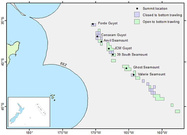
Figure 1. Location of the surveyed seamounts and guyots within the Louisville Seamount Chain. Dots mark the location of the seamount summit, boxes mark areas open/closed to New Zealand bottom fishing. Inset image shows the location of the study area in relation to New Zealand.

Seven large seamounts in the Louisville Seamount Chain were selected for survey (Forde, CenSeam, Anvil, JCM, 39 South, Ghost, Valerie) (Figure 1) with the aim to represent as wide a geographic range as possible given the available survey time. All seven seamounts have a vertical elevation of more than 1 km from the surrounding seafloor, and summary details for each are given in Table 1. Among the chosen seamounts there is a general gradient of increasing historical bottom trawling from north to south. Bottom trawling has taken place on all these seamounts and much of the area (excluding Forde and CenSeam) remains open to fishing by New Zealand bottom trawlers under SPRFMO regulations. These regulations control fishing in designated 20-min latitude/longitude blocks by vessels flagged to SPRFMO Member States. Regulations are based on a “bottom fishing footprint” established during the 2002-06 SPRFMO reference period (SPRFMO CMM2.03, https://www.sprfmo.int/), and for New Zealand vessels these are subject to open, move-on, and closed rules (Penney et al., 2009) (Figure 1).

TABLE 1

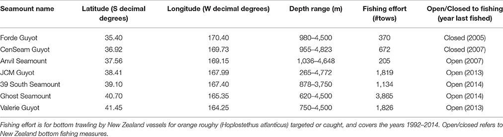
Table 1. Summary details of the surveyed seamounts.

Sampling

A random-stratified survey of benthic fauna and habitats using a towed camera system and an epibenthic sledge was undertaken on each study seamount to test the abilities of two broad-scale models to predict the presence of reef-forming corals (Anderson et al., 2016a). Data collected during this survey were also intended to enable subsequent development of high-resolution habitat suitability models at the scale of individual seamounts in the present study. Clark et al. (2015) and Anderson et al. (2016a) describe the survey design and sampling methodology in detail, but some of this information is repeated here for completeness.

Prior to running photographic transects, a multibeam echosounder (MBES) survey was conducted on each seamount (except Anvil where existing data were available) using a 30 KHz Kongsberg EM302, producing a data resolution of 25 × 25 m. Each photographic transect was ~1.4 km long (mean ± SD, 1.43 ± 0.27) and 2 m wide, and some targeted epibenthic sled deployments were made along the video transects to collect physical samples for verification of visual identifications and other research. Photographic transects were carried out using NIWA's deep towed imaging system (DTIS, Hill, 2009), which incorporates high definition video (Sony HD 1080i format) and still camera (Canon 10MP single lens reflex) systems, with an ultra-short baseline positioning system (USBL, Kongsberg HiPAP) for tracking and recording the precise seabed position of the equipment (accurate under ideal conditions to within 1 m). In total, 118 photographic transects were completed, with 20, 22, 13, 1, 17, 29, and 16 on Forde, CenSeam, Anvil, JCM, 39 South, Ghost and Valerie seamounts, respectively (Figure 2).

FIGURE 2

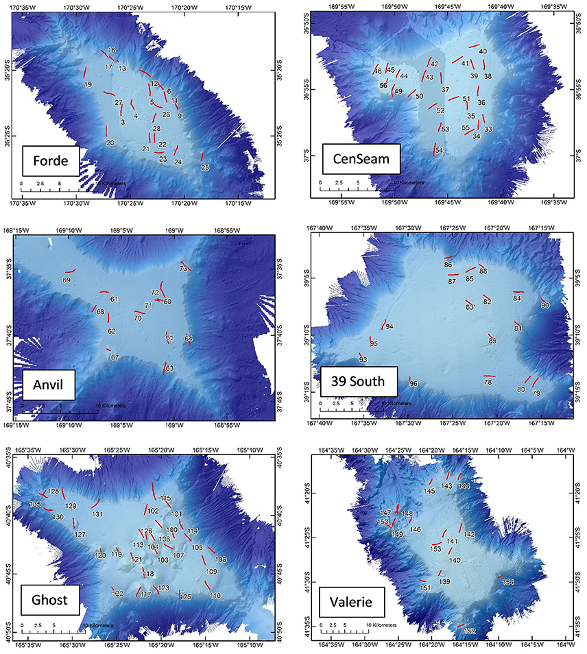
Figure 2. Bathymetric maps showing the position of photographic transects on each of the study seamounts (number = station number). JCM seamount is not shown because it was only partially surveyed and only one photographic transect was completed.

Data and Data Processing

Identifications and counts of fauna observed in video transects were made in real-time via a low-resolution video link to the ship, and from later analysis of full-resolution video for selected transects in which VME indicator taxa (primarily stony corals) occurred. S. variabilis was the only significant habitat-forming coral observed in the study area. Because much of the S. variabilis matrix of colonies observed was evidently not alive (dark colouration with no feeding polyps visible in high resolution still imagery), occurrence of this taxon was recorded in two ways: as percent cover of the seabed by intact coral matrix (“intact coral”), and counts of distinct coral colonies or “heads” with live polyps (“live heads”). The occurrence of non-intact coral matrix (broken up coral colonies that can occur around intact coral) was not recorded. Abundance data were then extracted for the three study taxa: live heads of S. variabilis; brisingid starfishes (Order Brisingida), and sea-lilies and feather stars (Class Crinoidea). The first species belongs to the VME indicator taxon Order Scleractinia, while the latter two are VME habitat indicator taxa for coral reefs (sensu Parker et al., 2009). Abundances were recorded as the number of individuals (or live heads) per 25 m² segment of video transect (~2 m transect image width × 12 m along the transect track).

A working definition of VME coral reef habitat, as opposed to individual occurrence of S. variabilis, was derived from video observations in the context of: (a) guidelines on identifying “sensitive environments” in the New Zealand region (schedule 6, Exclusive Economic Zone and Continental Shelf (Environmental Effects—Permitted Activities) Regulations 2013 http://www.mfe.govt.nz/marine/legislation/regulations-under-eez-act) and (b) our intuitive evaluation of VME status from observation of the seabed video imagery during the voyage and post-voyage confirmation from high-resolution imagery. According to the guidelines, “stony coral thicket or reef” habitat (Figure 3A) exists where either live or dead colonies of a structure-forming coral taxon cover more than 15% of the seabed over areas of >100 m². Using this as a starting point, for each 25 m² video segment, we calculated the proportion of the seabed identified as intact coral. To approximate to ~100 m², we then identified areas along each transect where any 3 or more segments in a 5-segment moving window had more than 15% intact coral. We then compared a number of possible formulations for VME definition (excluding extensive areas of dead coral matrix), each incorporating different measures of the numbers of live S. variabilis heads, against our intuitive evaluation of VME status. The definition (“rule”) that best matched our intuitive evaluation combined only two criteria: (1) more than 15% intact coral present in 3 or more segments of a 5-segment moving window, and (2) more than one live S. variabilis head present in 3 or more segments of the 5-segment moving window. Having arrived at this definition of VME habitat status, we then calculated the mean number of live S. variabilis heads per VME habitat segment per transect for each transect in which VME habitat occurred, and then took the lowest mean value obtained (2.78 S. variabilis live heads per VME habitat segment, transect #135) as a threshold indicator of VME coral reef habitat (Figure 3B). This abundance threshold value was applied to the outputs from the suitability modeling (see below) to map the predicted distribution of VME habitat.

FIGURE 3

Figure 3. (A) Seabed photograph showing coral reef habitat (live coral heads are lighter colored) and associated fauna including brisingids and crinoids (station 150, Valerie Guyot). (B) Illustration of VME habitat definition approach based on video transect observations, showing the occurrence of: all intact Solensmilia variabilis colony matrix (“intact coral”); VME coral reef habitat as defined by a “rule” (“VME by rule,” see methods text), and an abundance indicator of VME coral reef habitat (“live coral head threshold”) based only on a minimum threshold for live Solensmilia variabilis heads derived from their occurrence in the “VME by rule” areas. Black lines show full video transect paths (numbers = station number). This example is from the northwest flank of Ghost Seamount.

A set of more than 100 topographical terrain variables was derived from bathymetric data collected by the MBES survey using Benthic Terrain Modeler in ArcGIS 10.3.1 (ESRI, 2015). Terrain variables included those that have been shown previously to be useful for predicting suitable habitat for VME indicator taxa (e.g., Rengstorf et al., 2012). The continuous variables were: depth; slope (steepest gradient to any neighboring cell); aspect (direction of slope); curvature (change of slope); plan curvature (curvature of the surface perpendicular to the slope direction); and profile curvature (curvature of the surface in the direction of slope). In addition, a further set of derivative continuous variables were calculated using focal mean analysis in ArcGIS for the standard deviation of depth, depth range, standard deviation of the slope, and terrain ruggedness. Focal mean analysis finds the average value of a variable within a specified neighborhood centered on a given cell and outputs these data to the corresponding cell location. Four different neighborhood sizes (3 × 3, 5 × 5, 7 × 7, and 15 × 15 grid cells) were computed to produce more generalized datasets. The different neighborhood cell sizes were selected to mimic a range of spatial scales at which seafloor bathymetry and topography may affect the distribution of benthic communities (e.g., 3 × 3 cells = 75 × 75 m; 5 × 5 = 125 × 125 m; 7 × 7 = 175 × 175 m; 15 × 15 = 375 × 375 m). Aspect, measured continuously in degrees, was transformed into a categorical variable representing the 16 sectors of the compass (i.e., N, NNE, NE, etc).

Backscatter data from the MBES survey were processed using SonarScope (Augustin and Lurton, 2005). Processing consisted of statistical compensation of the signal as a function of its incidence angle on the seafloor, to attenuate the strong signal from specular reflection at the nadir and the rapid decrease of the signal strength with increasing incidence angle (Fonseca et al., 2009). Backscatter strength (a continuous variable), which measures the acoustic reflectivity of the seafloor, has been found to be a useful surrogate for substratum type (Lamarche et al., 2011). Substratum type influences the distribution of benthic organisms, including the study taxa which typically occupy hard substratum (high backscatter seafloor), and backscatter strength has been related to the distribution of deepwater coral species in previous studies (e.g., Georgian et al., 2014).

Because backscatter data were not available from the earlier MBES survey of Anvil Seamount, this seamount was excluded from modeling. JCM Seamount was also excluded because only a part of the seamount was surveyed using MBES, and only one photographic transect was completed on the feature. That is, only models for five out of the original seven seamounts surveyed were made. Some biological data from the two excluded seamounts is presented later.

Model Types and Selected Model Settings

We selected three statistical modeling methods in common usage for habitat suitability modeling; Boosted Regression Trees, General Additive Models, and Random Forests. Model predictions of habitat suitability across all seamounts were restricted to a maximum depth of 2,000 m (the depth limit of the video survey) and a minimum depth of 265 m (the summit of the shallowest seamount).

Boosted Regression Tree (BRT)

Boosted Regression Tree (BRT) modeling is an approach which can utilize both presence-absence data and abundance data, and has been used previously to predict distributions of deep-sea taxa in the study region (Anderson et al., 2016a,b). BRT models incorporate recursive binary splits within a regression tree structure to explain the relationship between the response and predictor variables (Elith et al., 2008). BRT models were fitted in R (R Development Core Team, 2016) using a standard approach, including optimization of the learning rate and number of trees by internal cross validation (Elith et al., 2008), and setting tree-complexity to 3 to allow a level of interactions between terms. The minimum number of trees for each model was set at 700. For construction of presence-absence models a Bernoulli (= binomial) distribution was assumed and for abundance models (count data) a Poisson distribution was assumed. Other model settings were left at default values.

A Generalized Additive Model (GAM)

A Generalized Additive Model (GAM) is a specific form of a generalized linear model that estimates smooth, non-parametric functions for each predictor variable (Hastie and Tibshirani, 1986). The distributions of a number of deep-sea species have been successfully modeled using a GAM approach, including corals (Rooper et al., 2014; Murillo et al., 2016), sponges (Rooper et al., 2014; Murillo et al., 2016), and fish (Leathwick et al., 2006). GAMs were developed in R using the “mgcv” package (Wood, 2006). For presence-absence models, a binomial distribution was assumed during model construction. For abundance models, a zero-inflated Poisson distribution with no data transformation was selected after exploring several alternative distributions (Gaussian, Poisson, quasi-Poisson, and Tweedie) and transformations (log+1, log+1% of mean abundance, square root, and fourth root) through analysis of residuals and model deviance. For all models, predictors were fitted with smooth terms allowing up to 4 degrees of freedom.

Random Forest (RF)

Random Forest (RF) modeling (Breiman, 2001) is a non-parametric approach which builds classification trees (presence-absence data) or regression trees (abundance data) using random subsets of the input data. One potential benefit of random forest over modeling approaches such as GAMs is the lack of any underlying assumption of the distribution of the response variable. RF models were constructed using the “randomForest” package (Liaw and Wiener, 2002) in R. For all models, 501 trees were run, which was always sufficient to allow the error rate to stabilize. Different values of “mtry,” the number of variables used in each tree node, were explored during initial model construction using the “tuneRF” function in the “randomForest” package. Default values (square root of the number of environmental variables for classification models, 1/3 the number of environmental variables for regression models), consistently produced the best results and were used in all models. Classification trees are highly sensitive to imbalances in the response variable, as the model will minimize the overall error rate at the expense of the error rate of the minority class (Chen et al., 2004; Evans et al., 2011). As our taxa data were skewed (>10:1 ratio of absences to presences for all species), we set the “cutoff” parameter in “randomForest” equal to species prevalence for each presence-absence model (Guo et al., 2004), which greatly reduced omission errors without affecting overall model performance.

Model Performance and Precision

Model performance was assessed using a cross-validation procedure in which models were trained using a random partition of data (70%) and tested against the remaining portion (30%). This cross-validation was carried out for 10 test datasets derived from different combinations of extracted data. For presence-absence models the area under the curve (AUC) metric was assessed for each of the ten test datasets, and an average calculated. In general, AUC values of ≥0.5 indicate better than random performance, ≥0.7 indicate adequate performance, and ≥0.8 indicate excellent performance (Hosmer et al., 2013). For abundance models, correlations (R²) between predicted and observed values for the 10 test datasets were calculated, and averaged. In addition, for both presence-absence and abundance models (and ensemble models—see below), the correlation (R²) between predicted and observed values was calculated for the whole dataset. For presence-absence models this was achieved by first converting model probabilities into a binomial form comparable with the observed data using cut-offs which provided an equivalent number of presences and absences. In all cases the final models were constructed using all data.

In order to assess the relative confidence in predictions across the model extent, we used a bootstrap technique for each model type to produce spatially explicit uncertainty measures, after Anderson et al. (2016b). Random samples of the input data, in which presence and absence records were in equal proportion and number to the original (for both presence-absence and abundance models) were drawn with replacement, and models constructed with the same settings as the original. Predictions were then made for each cell of the model extent. This process was repeated 500 times for BRT models and 200 times for GAM and RF models (limited by processing capacity) resulting in 500 or 200 estimates for each cell. We then calculated model uncertainties as the coefficient of variation (CV) of the bootstrap output.

Ensemble Models

Fundamental differences in model structure among the three models will inevitably result in different patterns of predicted habitat suitability. Evaluations of different types of models are often unable to demonstrate the unequivocal superiority of any single type, and studies have shown that predictions by alternative models can be so variable that they compromise their use for guiding policy or decision making; a solution to this issue is to use “ensemble” models (Araújo and New, 2007). Hence, for incorporation into decision-making tools for spatial management planning (e.g., Zonation, Moilanen, 2007) an ensemble model is a practical way to avoid dependence on a single model type and better describe in general the predicted spatial variation and uncertainties (Robert et al., 2016). To incorporate the predictions and underlying assumptions of each model into a single output grid we produced ensemble models of presence-absence and abundance, by calculating weighted averages of the relevant BRT, GAM, and RF models (after Oppel et al., 2012 and Anderson et al., 2016b).

$\begin{array}{l}{W}_B=\frac{P{S}_B}{P{S}_B+P{S}_G+P{S}_R},W_G=\frac{P{S}_G}{P{S}_B+P{S}_G+P{S}_R},\text{ and}\\ W_R=\frac{P{S}_R}{P{S}_B+P{S}_G+P{S}_R}\\ X_E=X_B*W_B+X_G*W_G+X_R*W_R\\ C{V}_E=\sqrt{\frac{{(C{V}_B*X_B)}^2*W_B^2+{(C{V}_G*X_G)}^2*W_G^2+{(C{V}_R+X_R)}^2*W_R^2}{X_E^2}}\end{array}$

where PS_B, PS_G, and PS_R are the model performance statistics (AUC for presence-absence models and R² values for abundance models); X_B, X_G, X_R, and X_E the model predictions; and CV_B, CV_M, CV_G, and CV_E the bootstrap CVs from the BRT, GAM, and RF, and ensemble models respectively.

Precision estimates for the ensemble models were calculated as the correlation (R²) between predicted and observed values calculated for the whole dataset, as described above.

Predictor Variable Selection

The topographical terrain and backscatter variables derived from the MBES survey formed the basis of the model predictor variable set. Chemical and other water property variables, including biological productivity variables available from various global or regional climatologies, were not considered as none were available with a native resolution similar to that of the MBES-derived variables. Several of these variables (e.g., temperature, salinity, surface-derived production, and aragonite saturation) are correlated with depth to varying degrees, and so a depth variable in this case can act as a surrogate for the changes in these parameters (Leathwick et al., 2006; Thresher et al., 2014). The categorical variable seamount, identifying the individual seamounts, was however added to MBES-derived candidate variables. Seamount was used rather than latitude and longitude to predict potential geographic-related environmental differences in habitat suitability, because this variable could also be used to reflect variables that may be specific to a particular seamount that are not related simply to geography.

The full set of candidate variables was initially reduced by eliminating highly correlated variables, based on Pearson product-moment correlation coefficients. Values for the remaining variables were then determined for the midpoint locations of each of the 25 m² taxa presence/absence video segments and used to build a set of single-variable presence-absence GAM models for each of the three taxa, as well as models using all of the variables together. The predictive value of each variable was then assessed according to its chi-square score in the all-variable models, and its AUC score in the single-variable models. In order to further assess the relative utility of the remaining candidate variables, we considered relationships among them using a cluster dendrogram, again using Pearson product-moment correlation coefficients. In this way priority was given to variables that had low correlations with other variables and occurred in unique clusters, so as to avoid losing information that was not also provided by other variables, and to avoid including only high-performing variables that provided similar information.

Moran's index was used, with the “spdep” package for R (Bivand, 2011), to measure spatial autocorrelation in model residuals compared with the raw presence-absence or abundance data. This index measures the correlation between observations as a function of the distance separating them, with values between−1 (highly dispersed) and 1 (highly clustered).

In order to account for the inherent spatial autocorrelation in the model data, where relationships between observations are correlated with the geographic distances between them, we created an additional predictor, the residual autocovariate (RAC), representing the similarity between the residual from initial models at a location compared with those of neighboring locations. This method can account for spatial autocorrelation without compromising model performance, and can easily be implemented in most modeling approaches (Crase et al., 2012).

Model Outputs

All model results [predicted probability of occurrence/suitable habitat [0–1] and predicted abundance [number 25m⁻²] for each model and taxon, and the corresponding coefficients of variation (CV)] were mapped onto the newly derived bathymetry for the seamounts using ArcMap 10.3.1 (ESRI, 2015) at the same spatial resolution as the model environmental input data (25 × 25 m). Maps were drawn with a constant probability/abundance scale between models and taxa so that visual comparisons can be easily made.

As a measure of the utility of the two VME habitat indicator taxa Brisingida and Crinoida for identifying the location of stony coral VME habitat, correlations between the predicted abundance of S. variabilis and the predicted abundance of these taxa were calculated from the ensemble-abundance model outputs.

Results

Photographic Transects

The stony coral S. variabilis and brisingids were present in less than 500 of the 12,504 25 m² video segments observed. Crinoids were two–three times more common across all seamounts, but this taxon was represented by a greater number of species than the other VME habitat indicator taxon (Table 2, Figure S1). During the survey, at least 11 species of crinoids were identified from samples collected using the epibenthic sled (the comatulids Aglaometra incerta, Charitometra basicurva, Florometra novaezealandiae, Glyptometra inaequalis, Antedon sp., Crotalometra sp., Cyclometra sp., Porphyrocrinus sp., Strotometra sp., and the hyocrinid Thalassocrinus, sp. plus several unidentified comatulids), compared with three species of brisingids (Novodinia novaezelandiae, Freyella sp., and Hymenodiscus sp.).

TABLE 2

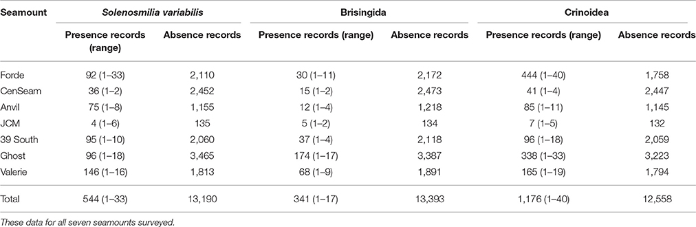
Table 2. VME indicator and habitat indicator taxa, the number of presence and absence records, and for presence records, the minimum and maximum number of records per video transect segment (25 m²).

Variable Selection

Related variables based on a single focal mean neighborhood size (e.g., the range and standard deviation of curvature, curvature aspect, and plan curvature) were often highly correlated (>75%). Correlations between these variables and all remaining variables were examined graphically to eliminate all but the least correlated of them. Similarly, ruggedness was highly correlated with standard deviation of slope, and the latter variable was eliminated due to its higher correlation with other retained variables. This logic was followed for all variable types and focal mean neighborhood sizes to eliminate the most correlated variables, reducing the set of more than 100 MBES-derived variables to 63.

Chi-square values for the GAM models based on all 63 remaining variables, and AUC scores for 63 single-variable models (for each taxon) revealed a consistent set of eight variables which showed a high level of explanatory power while covering a range of the variable types derivable from MBES data. Cluster dendrograms and correlation coefficients showed clustering of these variables and no two variables were more than 70% correlated (Figures S2, S3).

Separate RAC variables were constructed for each model type (BRT, GAM, and RF), prediction type (presence-absence and abundance), and taxon (S. variabilis, Brisingida, and Crinoidea), based on the residuals from initial models constructed from the eight MBES-derived variables. The final set of nine variables used in each of the models is shown in Table 3.

TABLE 3

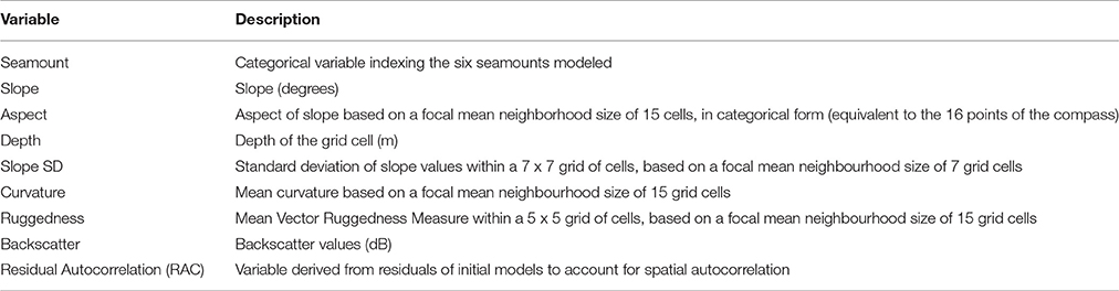
Table 3. Final set of predictor variables used in the habitat suitability models.

Model Performance

Cross-validated AUC values were very similar for each of the presence-absence models, ranging between 0.90 and 0.93 in all cases except for the Brisingida GAM model which was lower (0.87) but still considered excellent (Hosmer et al., 2013) (Table 4). The generally similar AUC values among the three model types for each taxon meant that there was a similar weighting, and therefore a similar influence, for each model in the ensemble models. Overall, and consistently across the three taxa, RF models performed slightly better than BRT models, and GAM models performed worst according to cross validated AUC. Correlations (R²) between predicted and observed presence-absence for all model data showed broad agreement with the AUC performance measures, although they were consistently slightly higher for BRT models (26.6–37.8%) than for RF models (23.7–33.7%), and considerably lower for GAM models (7.5–16.0%). Among the three taxa, the model performance was highest for S. variabilis and Crinoidea, and lowest for Brisingida, according to both the AUC and correlation statistics. The performance measures (correlation only) for the ensemble models reflect the mean performance of the three contributing models, and do not directly assess their ability to predict outside observed cells.

TABLE 4

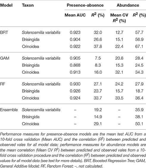
Table 4. Comparison of performance statistics for four types of presence-absence and abundance models for Solenosmilia variabilis, Brisingida, and Crinoidea on seamounts of the Louisville Seamount Chain.

For the abundance models, cross validated correlations (Mean CV R²) were lowest overall for Brisingida but similar among the three model types (15.1–15.7%); they were more variable for S. variabilis (from 12.7% for BRT to 24.2% for RF) and consistently highest for Crinoidea (22.4–33.5%). By this measure GAM and RF models performed similarly well, and consistently better than BRT models. Correlations (R²) between predicted and observed presence-absence for all model data were highest for BRT models (56.9–67.1%) and similar for RF and GAM models (18.7–36.4%). By this measure the models for Crinoida again consistently performed better than those for the other two taxa. The all-data correlation values were considerably higher for abundance models compared with presence-absence models for BRT and GAM models (24.5–67.1%), but similar for RF models. By this measure BRT models (and the ensemble models) performed better than RF and GAM models.

Predictor Influence

For all model types, autocorrelation in the residuals (measured using Moran's index) was substantially reduced with the inclusion of the RAC variable. The RAC variable had the greatest influence in all models except for the abundance model for Crinoidea (Table 5). The most influential environmental variable in all the BRT models was Aspect, with a tendency for higher abundance and presence on westerly sector slopes. In contrast, for the GAM and RF models there was no single consistently important environmental variable for all indicator taxa and the two types of models. The variable SlopeSD was the most important for GAM presence-absence and abundance models for S. variabilis, while Curvature and Slope were the most important variables for Brisingida and Crinoidea GAM models, respectively. Slope SD and Depth were the two most important environmental variables for RF models of S. variabilis, while Backscatter was more important for the abundance model of this species. Slope SD and Curvature were the most important environmental variables for RF models of Brisingida presence-absence and abundance, respectively. For RF models of Crinoidea, Slope was the most important variable. The least important environmental variables also varied among BRT, GAM, and RF models for VME indicator taxa and the two model types, but Seamount, Backscatter and Aspect (with the exception of the BRT models) were most often the least important variables (Table 5). See Figure S4 for details of the influence of the predictor variables across their full range in the model data.

TABLE 5

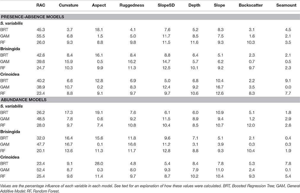
Table 5. Variable contributions to each type of habitat suitability model for each VME indicator taxon.

Habitat Suitability Predictions

Generally across all seamounts, the distribution of suitable habitat (≥0.5 probability of occurrence for presence-absence models and >0.5 live coral heads per 25 × 25 m grid cell for abundance models; thresholds = more likely to occur than not, and relatively high abundance, respectively) was predicted to be more extensive by the BRT models than either the GAM or RF models, although the basic distribution patterns were similar. Differences between the models were more pronounced in the presence-absence models than the abundance models. The distribution of suitable habitat predicted by the ensemble models for all taxa reflected the underlying averaging principle of this approach (e.g., Figures 4A,B for Forde Guyot; see Figure S5 for comparison among model types for other seamounts).

FIGURE 4

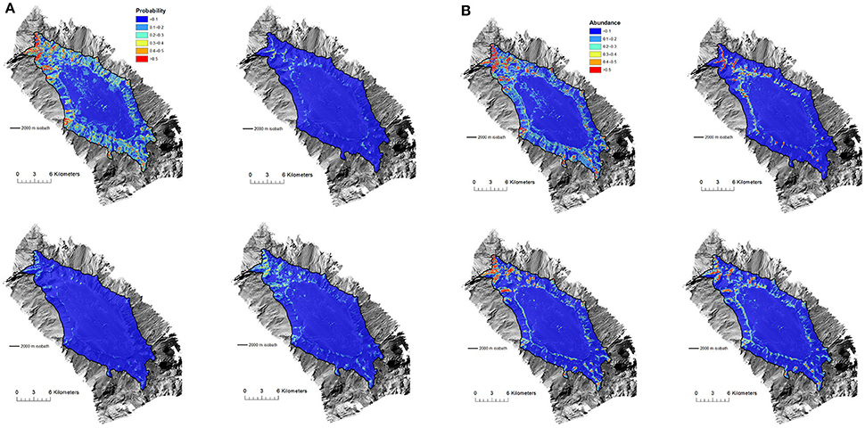
Figure 4. (A) Forde Guyot. Model predictions of Solenosmilia variabilis habitat suitability (probability of presence) showing difference between model types (top left, BRT; top right, GAM; bottom left, RF; bottom right, Ensemble). Color-coded model probabilities are draped over the MBES bathymetry obtained during the survey. (B) Forde Guyot. Model predictions of Solenosmilia variabilis abundance (number of “live head” colonies per 25 × 25 m model cell) showing difference between model types (top left, BRT; top right, GAM; bottom left, RF; bottom right, Ensemble). Color-coded model abundance estimates are draped over the MBES bathymetry obtained during the survey.

Because the abundance models performed better than presence-absence models, and ensemble models are practical for spatial management planning purposes (to avoid dependence on single model types), only the habitat suitability results of the ensemble-abundance models are described in detail hereafter. All the results of the other models are provided in Figure S5.

Suitable habitat for S. variabilis was generally predicted to occur at the summit-slope break, and on ridge-like features that extended down the flanks of the seamounts. Some areas of the seamount flanks were predicted to have concentrations of suitable habitat for this coral. Generally, these areas were on the north and north-west flanks of the seamounts. Where they occurred (particularly on Ghost Seamount), isolated knoll-like features on the flat summits of seamounts were also sometimes predicted to have suitable habitat for S. variabilis (Figure 5).

FIGURE 5

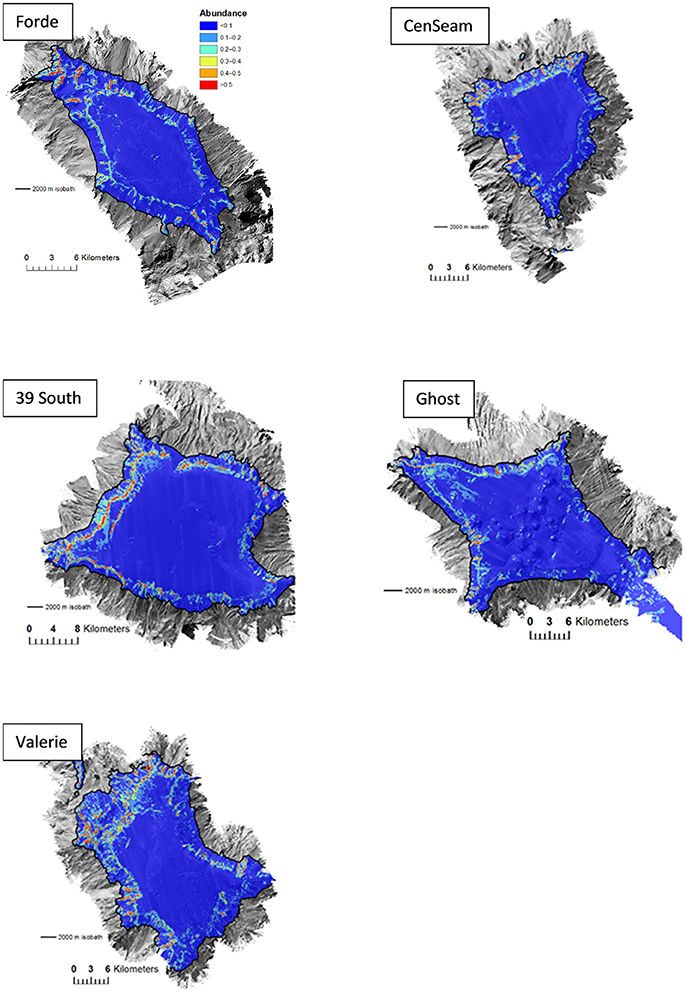
Figure 5. Predictions of Solenosmilia variabilis abundance (number of “live head” colonies per 25 × 25 m model cell) for ensemble habitat suitability model. Color-coded model abundance estimates are draped over the MBES bathymetry obtained during the survey.

The distribution patterns of suitable habitat predicted by ensemble-abundance models for crinoids and brisingids were generally similar to those for S. variabilis across all seamounts (i.e., summit-slope break, ridges on flanks). However, highly suitable habitat for crinoids was more extensive than for brisingids on the seamount flanks (particularly on Forde Guyot where the mean number of crinoid observations per cell were over three times higher than for other seamounts) (Figure 6). Correlations varied between the ensemble-abundance models for the VME indicator taxa S. variabilis and the two taxa that are supposedly indicators of the habitat formed by the stony coral. The correlation between the models for Crinoidea was relatively high (R = 0.53), compared to that for Brisingida (R = 0.25).

FIGURE 6

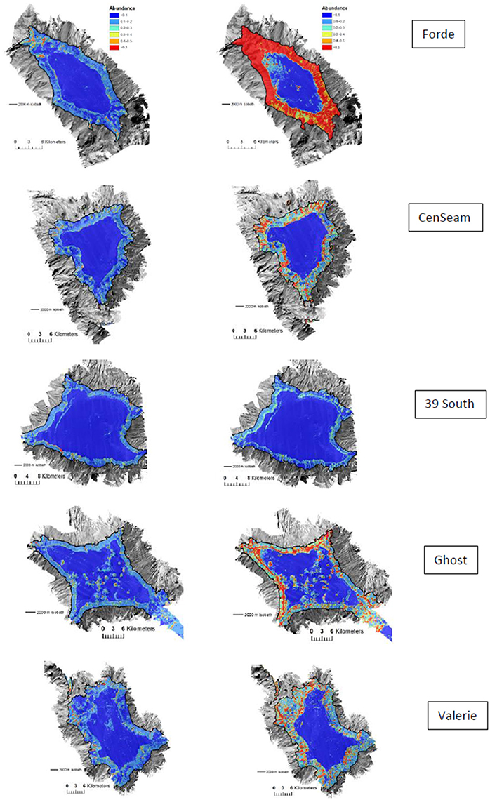
Figure 6. Predictions of brisingids (Left) and crinoids (Right) abundance (number per 25 × 25 m model cell) for ensemble habitat suitability model. Color-coded model abundance estimates are draped over the MBES bathymetry obtained during the survey.

Uncertainty

Spatial patterns of model uncertainty varied among BRT, GAM, and RF models, but these patterns were generally similar between presence-absence and abundance models. Highest levels of uncertainty were generally associated with areas of highest habitat suitability for BRT models (i.e., seamount flanks), low habitat suitability at the deepest depths for GAM models (i.e., base of seamount flanks), and low habitat suitability at the shallowest depths for RF models (i.e., the flat seamount summit). Uncertainty for ensemble models was lower overall compared to the other models, and where areas of relatively high uncertainty occurred for ensemble models they were limited to small patches on the flanks of the seamounts (e.g., Figure 7 abundance models for S. variabilis on Forde Guyot; see Figure S5 for all models for other taxa and seamounts).

FIGURE 7

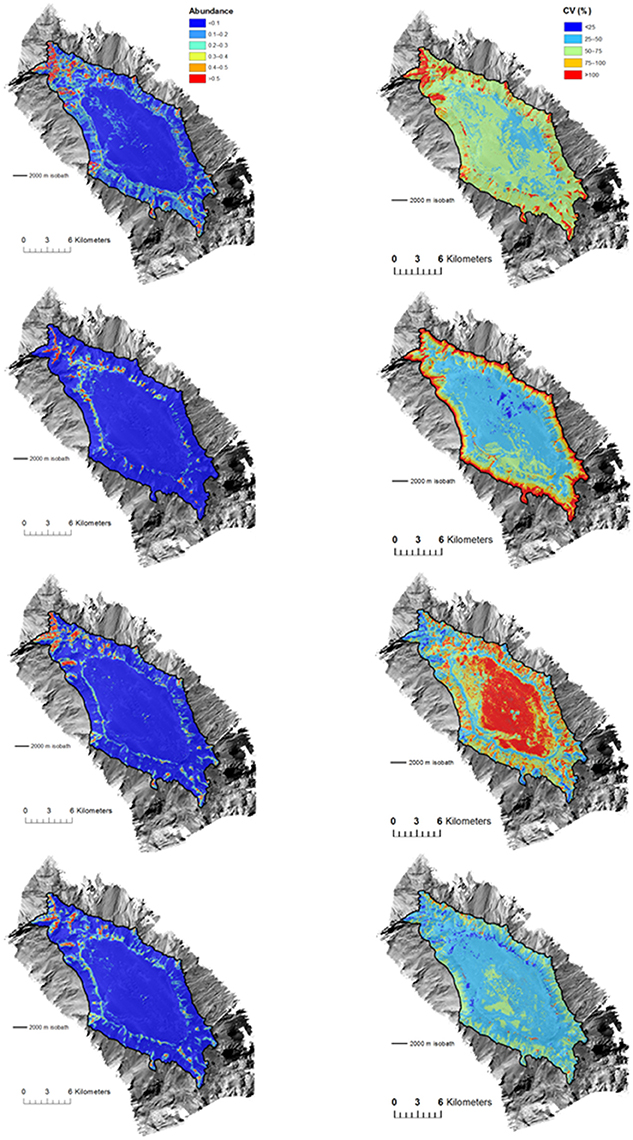
Figure 7. Forde Guyot. Prediction of Solenosmilia variabilis (Left) abundance (number of “live head” colonies per 25 × 25 m model cell) and (Right) uncertainty (CV) for (from top to bottom) BRT, GAM, RF, and ensemble habitat suitability models. Color-coded model abundance estimates and CV are draped over the MBES bathymetry obtained during the survey.

Distribution Predictions for Coral Reef VME Habitat

The ensemble-abundance models for coral reefs predicted that this VME habitat was sparsely distributed on all seamounts (Figure 8). Where it was predicted to occur at the summit-slope break and ridges on the seamount flanks, the patch size of this habitat was typically small with few relatively large patches (range from 625 to 42,500 m²), and did not total more than 0.6 km² or 0.09% of the modeled area of any single seamount (Table 6, Figure 9).

FIGURE 8

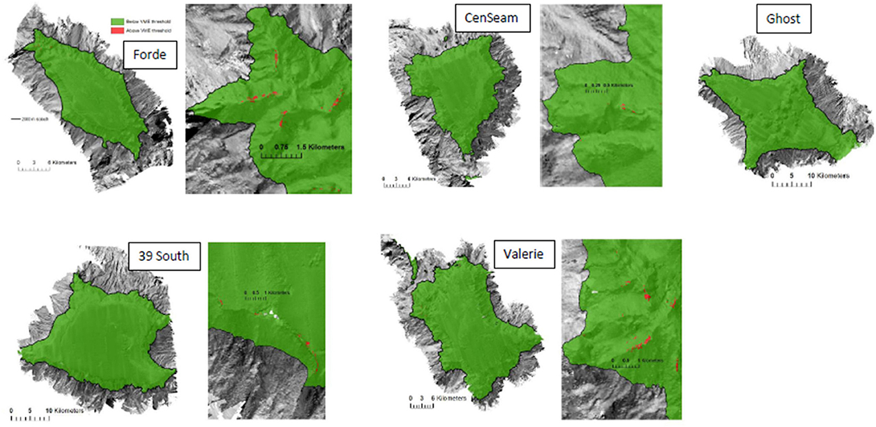
Figure 8. Predictions for coral reef habitat based on VME threshold (“live coral head threshold”; see Methods text for explanation). Enlargements show the predicted distribution of coral reef habitat patches on the part of the seamount where they are most prevalent (apart from Ghost, where patches were not concentrated in one area). Maps are draped over the MBES bathymetry obtained during the survey.

TABLE 6

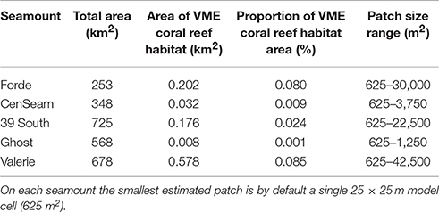
Table 6. Total seamount area within the modeled depth range (265–2,000 m), estimated area and proportion of VME coral reef habitat, and range of VME habitat patch size.

FIGURE 9

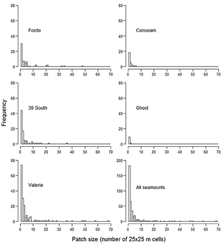
Figure 9. Distribution of predicted VME coral reef habitat patch sizes on individual seamounts and overall.

Discussion

The results of our study contribute to the growing number of examples that demonstrate the potential for using high-resolution habitat suitability models for the conservation and management of VMEs in the deep sea. Our models predict that suitable habitat for the stony coral VME indicator species S. variabilis is found at distinct breaks in slope and on elevated ridge-like features on seamounts. The general pattern of distribution predicted by our models conforms to expectations from previous observations of the distribution of stony corals at seamounts, canyons and continental slopes, and the topographic-related factors that are thought to control their distribution at these locations (e.g., Frederiksen et al., 1992; Thiem et al., 2006; Reveillaud et al., 2008). The predicted small-scale distribution patterns for S. variabilis, and the topographic variables identified as being important in these models (Aspect, Slope, SlopeSD, Curvature), are similar to those resulting from previous habitat suitability models for similar coral species found elsewhere (e.g., Dolan et al., 2008; Howell et al., 2011; Rengstorf et al., 2012).

Habitat suitability models for crinoids and brisingids, taxa that are considered to be indicators of VME habitat (Parker et al., 2009), were correlated with those for the stony coral S. variabilis. However, the correlations were not strong, particularly for brisingids. As such, in a habitat suitability modeling context, these taxa are not likely to be useful model proxies for the presence of coral habitat. Many observations suggest an association between the occurrence of crinoids and brisingids and the stony coral, and the contribution of their presence to the “VME indicator score” used by observers on fishing vessels operating the “move-on rule” (Parker et al., 2009) appears to be supported to some extent by the present study. However, despite their co-occurrence with stony corals in areas of high relief and hard substrate, there is also a growing body of data showing that both of these taxa can occur on bare rock surfaces, and that Brisingids can occur on soft sediment seabeds.

Below we discuss the results of our study with particular reference to improving high-resolution habitat suitability modeling, identifying and mapping VME habitat, and implications for spatial management in the SPRFMO Convention Area. For discussion about the limitations of the model types and general modeling methodology used in this study, please see Anderson et al. (2016b).

High-Resolution Habitat Suitability Mapping

The efficacy of habitat suitability modeling, using seafloor camera imagery and bathymetric and backscatter data obtained from multibeam surveys to make high-resolution predictive distribution maps for benthic species of conservation or management significance in the deep sea was first demonstrated off SW Ireland by Dolan et al. (2008). Since then similar models for VME indicator taxa have been made and developed for the same area and elsewhere in the NE Atlantic Ocean (Guinan et al., 2009; Howell et al., 2011; Rengstorf et al., 2012, 2013, 2014; Tong et al., 2013; Robert et al., 2016). However, none of these studies produced abundance-based models for VME indicator taxa, nor used measures of abundance to model directly the distribution of VME habitat.

Howell et al. (2011) modeled the distribution of the presence of the stony coral Lophelia pertusa and coral reef habitat, but the latter was based on data from the subjective identification of reefs by eye. Nonetheless, this study demonstrated the importance of distinguishing between models for VME indicator taxa and VME habitat, and the authors suggested that “mapping efforts should focus on the habitat rather than the species at fine (100 m) scales” (Howell et al., 2011). Robert et al. (2016) used quantitative density data in their high resolution models but did so indirectly by modeling the distribution of benthic assemblages (including a L. pertusa-dominated assemblage) that were first identified objectively using multivariate analyses based on abundance data for individual taxa. Their models also used the occurrence of coral and coral rubble substrata (classes derived from backscatter data) as predictor variables, and thus appear to include a degree of circularity (at least for predicting the occurrence of the L. pertusa-dominated assemblage). Rengstorf et al. (2014) used species occurrence proportion data for L. pertusa (i.e., number of presence records compared to the number of absence records in a grid cell) as a measure of coral prevalence. While they did not use abundance data in their models, they nonetheless found that models that included the semi-quantitative proportional data performed better than models based on presence-absence data, had lower coefficients of uncertainty, and were considered more reliable (Rengstorf et al., 2014).

Rengstorf et al. (2014) advocated the use of proportion data because of the time-consuming nature of obtaining true abundance data for benthic taxa from seabed imagery. However, where abundance data are available, they can significantly improve model performance and provide a more comprehensive understanding of spatial patterns, as clearly demonstrated by the present study.

Mapping VME Habitat

FAO (2009) notes that “merely detecting the presence of an element itself (i.e., a VME indicator taxa) is not sufficient to identify a VME.” Thus, as well as model improvements for VME indicator taxa, abundance data also offer the prospect of making distribution models for VME habitat based on a density threshold for habitat-forming taxa, rather than using data based solely on subjectively identifying VME habitat, or data for benthic assemblages that act as a proxy for VME habitat. However, VME habitat is not always or consistently defined by the density of the habitat-forming taxa. For example, definitions of coral reef habitat are not provided by FAO (2009) in their initial list of VMEs, and the longer description of coral reef habitats provided in support of the OSPAR List of Threatened and/or Declining Species and Habitats does not indicate any density or coverage thresholds (Hall-Spencer and Stehfest, 2009). In the few studies where deep-sea coral reef habitats are identified based on a particular density or coverage in a VME mapping context, values differ depending on the type of coral habitat. For example, Vertino et al. (2010) defined 20–40% coverage of dead and/or live coral colonies per video frame (~2.4 m²) for “Coral framework and hardground” habitat compared with >60% coverage for “Coral framework” habitat. These threshold-based identifications of VME habitat often include both dead and live corals, which reflects the typical composition of coral reef habitats. The amount of dead coral can be extensive, as found in the present study, by Thresher et al. (2011) off Tasmania, and by Vertino et al. (2010) in the Mediterranean where they noted live colonies rarely cover more than 30% of the seafloor. In the present study we constructed predictive maps of VME habitat based on the definition for coral reefs and thickets (as “sensitive environments”) provided by the regulations associated with New Zealand's EEZ Environmental Effects Act. However, this threshold-based definition is essentially a subjective regional translation of the “you know it when you see it” descriptions provided by the likes of OSPAR, rather than a density of corals determined directly from study of the structural or functional attributes that distinguish coral reefs as VMEs.

While our attempt to predict the distribution of VME habitat is currently defensible because no consensus exists about what density of corals is necessary to generate the structural and functional attributes of a VME, the lack of a robust density threshold-based definition of VME habitat potentially limits the acceptance of these maps for conservation and fisheries management purposes (see below). Nonetheless, the results of the present study are in line with the developments envisaged for habitat suitability modeling in order that predictive distribution maps can be better used for the spatial management of VMEs (Ross and Howell, 2013; Reiss et al., 2014; Rengstorf et al., 2014; Vierod et al., 2014; Robert et al., 2016). These improvements include our use of an abundance-based multi-model ensemble approach to produce high-resolution predictive distribution maps, and presentation of spatially explicit measures of model uncertainty for VME indicator taxa and VME habitat across a group of seamounts that are targeted by a specific fishery.

Implications for Spatial Management in the SPRFMO Convention Area

New Zealand deepwater fishing stakeholders have proposed that, because their bottom trawling occurs exclusively in relation to seamounts in the SPRFMO Convention Area, and that commercially viable fish concentrations vary within and between seamounts, as do presumably the abundance of benthic species, spatial management measures should be based on individual seamounts (https://www.sprfmo.int/assets/Meetings/Meetings-2013-plus/SC-Meetings/2nd-SC-Meeting-2014/Papers/SC-02-INF-04-Management-by-Seafloor-Feature-of-Deepwater-Fisheries-in-the-South-Pacific-Ocean-b.pdf). That is, open and closed areas should be defined on an individual seamount basis, with a sufficient fraction of each seamount closed to ensure adequate protection of VMEs. Fishing stakeholders have argued for this approach because they believe that spatial management based on large, regular shaped areas (e.g., areas defined by 20-min of latitude and longitude) precludes them from fishing areas within closed areas that are not suitable for VMEs, and that it is not necessary to impose large closure areas that might extend over most or all of a seamount. Furthermore, with the accurate deployment of fishing gear using modern navigational methods, it is possible to effectively avoid relatively small closed areas where it is known that VMEs do occur on a seamount. The fishing stakeholders accept that in order for this strategy to be implemented it is necessary to map the distribution of VMEs at high-resolution on each seamount within the broader fishing area. As we have demonstrated through the present study, habitat suitability modeling using multibeam data and seafloor images can achieve this mapping goal.

The ensemble habitat suitability models for S. variabilis predicted that concentrations of relatively high abundances of this VME indicator taxon typically occur in the north/northwestern areas of the seamounts, and sometimes in southern areas. However, relatively high abundances of the coral (>5 live heads 25 m⁻²) were predicted to occur around the entire seamount at the summit-slope break, mostly on ridge-like features that extend down slope from the flat top of the seamount summit (860–2,000 m—maximum modeled depth). This result suggests that only the flat topped and soft sediment summits are relatively large and discrete areas of consistently low habitat suitability for S. variabilis, and thus where bottom fishing could occur with a low likelihood of encountering this VME indicator taxon. However, these areas are not generally favored by fishers. Fishing patterns revealed by logbook data and commercial fishers plotter lines differ between seamounts, but indicate that fishers tend to target either small localized hill features on the summits (e.g., Ghost, 39 South), or the upper slopes and flanks of seamounts (e.g., Valerie, JCM) where over 90% of tows occur away from the summit plateau on the flanks to depths of 1,200 m. Our habitat suitability models predict that areas of relatively high abundance of S. variabilis are likely to be encountered by bottom trawling the seamount flanks. Based on the results of the abundance models for this VME indicator taxon, and current knowledge of the areas of interest to fishers, designing spatial management measures on an individual seamount level would be problematic.

The abundance models were also used to identify and predict coral reef habitat. This VME was predicted to occur as relatively small patches in only a few relatively isolated areas on seamounts. This limited distribution and abundance of VME habitat on seamounts conforms to the experience of the fishers, and thus supports one of their arguments for reducing the size of closed areas on seamounts, and adopting an individual seamount-based spatial management approach for the Louisville Seamount Chain. However, this conclusion is predicated on the veracity of the threshold-based approach by which VME habitat was identified in the present study. If predictive models are to be used for designing spatial management at the within-seamount scale, research is required to establish coverage and/or density estimates that relate to the specific structural and functional attributes that define a VME. For example, Cathelot et al. (2015) recently demonstrated that an area of 1,767 m² dominated by live corals with a density of visible live polyps of ~33 per 100 cm² can make a significant contribution to local ecosystem function in the deep sea. Some of the predicted coral reef habitat patches in the present study were greater than the size examined by Cathelot et al. (2015) (0, 18, 27, 38, and 41% of patches on the study seamounts were predicted to occupy ≥3 cells i.e., ≥1,875 m²) but most were smaller. So while it is probable that some of the coral reef habitat on the Louisville Seamounts Chain is providing important ecosystem function, the significance of the more numerous smaller patches of coral habitat is uncertain. The necessary patch size or polyp/live head density to represent significant sites of benthic respiration and organic carbon cycling, or significant habitat to support biodiversity or juvenile fish is unknown. Thus, we recommend that further research is needed to investigate and develop the way in which VME habitats are identified and included in habitat suitability modeling approaches (regardless of the resolution or spatial scale of the models) for the purpose of informing conservation and management. Such work should include multi-modeling approaches that incorporate the functional traits of species to improve the ecological interpretation of results, and support a broader ecosystem approach to management.

Author Contributions

AR and MC conceived of the study. AR, MC, and DB designed the field survey. MC, DB, OA, and AP collected data from the field survey. DB, AM, and AP analyzed image and multibeam data from the survey. OA and SG undertook the modeling. AR, OA, SG, MC, and DB interpreted all data. AR led the writing, and drafted text for the manuscript. OA, SG, MC, DB, and AP contributed draft text to the manuscript, and all authors revised and approved the final version of the manuscript.

Funding

This study is part of the NIWA-led South Pacific Vulnerable Marine Ecosystems Project funded by the New Zealand Ministry for Business, Innovation and Employment (C01X1229). Additional funding was provided by the Ministry for Primary Industries (ZBD201302).

Conflict of Interest Statement

The authors declare that the research was conducted in the absence of any commercial or financial relationships that could be construed as a potential conflict of interest.

Acknowledgments

Thanks are owed to the Captain, officers, crew, and scientific staff of the NIWA research voyage TAN1402, the survey that collected the data on which the study is based. Particular thanks are owed to Sophie Mormede (NIWA) and John Guinotte (MCI, USA) for assistance in the design of this survey, and to Chris Rooper (Alaska Fisheries Science Center, Seattle, USA) who provided useful modeling advice and code. This study also benefitted from advice and support provided by members of the project's Stakeholder Advisory Group.

Supplementary Material

The Supplementary Material for this article can be found online at: https://www.frontiersin.org/articles/10.3389/fmars.2017.00335/full#supplementary-material

References

Anderson, O. F., Guinotte, J. M., Rowden, A. A., Clark, M. R., Mormede, S., Davies, A. J., et al. (2016a). Field validation of habitat suitability models for vulnerable marine ecosystems in the South Pacific Ocean: implications for the use of broad-scale models in fisheries management. Ocean Coast. Manage. 120, 110–126. doi: 10.1016/j.ocecoaman.2015.11.025

CrossRef Full Text | Google Scholar

Anderson, O. F., Guinotte, J. M., Rowden, A. A., Tracey, D. M., Mackay, K. A., and Clark, M. R. (2016b). Habitat suitability models for predicting the occurrence of vulnerable marine ecosystems in the seas around New Zealand. Deep Sea Res. I 115, 265–292. doi: 10.1016/j.dsr.2016.07.006

CrossRef Full Text | Google Scholar

Araújo, M. B., and Guisan, A. (2006). Five (or so) challenges for species distribution modelling. J. Biogeogr. 33, 1677–1688. doi: 10.1111/j.1365-2699.2006.01584.x

CrossRef Full Text | Google Scholar

Araújo, M. B., and New, M. (2007). Ensemble forecasting of species distributions. Trends Ecol. Evol. 22, 42–47. doi: 10.1016/j.tree.2006.09.010

PubMed Abstract | CrossRef Full Text | Google Scholar

Ardron, J. A., Clark, M. R., Penney, A. J., Dunn, M. R., Dunstan, P. K., Watling, L. E., et al. (2014). A systematic approach to the identification and protection of vulnerable marine ecosystems. Mar. Policy 49, 146–154. doi: 10.1016/j.marpol.2013.11.017

CrossRef Full Text | Google Scholar

Augustin, J. M., and Lurton, X. (2005). Image Amplitude Calibration and Processing for Seafloor Mapping Sonars. Oceans 2005—Europe. Plouzané: IFREMER.

Google Scholar

Bivand, R. (2011). Spatial Dependence: Weighting Schemes, Statistics and Models. spdep_0.3-30.tar.gz.

Breiman, L. (2001). Random forests. Mach. Learn. 45, 5–32. doi: 10.1023/A:1010933404324

CrossRef Full Text | Google Scholar

Cathelot, C., Van Oevelen, D., Cox, T. J. S., Kutti, T., Lavaleye, M., Duineveld, G., et al. (2015). Cold-water coral reefs and adjacent sponge grounds: hotspots of bentghic respiration and organic carbon cycling in the deep sea. Front. Mar. Sci. 2:37. doi: 10.3389/fmars.2015.00037

CrossRef Full Text | Google Scholar

Chen, C., Liaw, A., and Breiman, L. (2004). Using Random Forest to Learn Imbalanced Data. University of California, Berkeley, CA.

Clark, M. R., Anderson, O., Bowden, D., Chin, C., George, S., Glasgow, D., et al. (2015). Vulnerable Marine Ecosystems of the Louisville Seamount CHAIN: Voyage Report of a Survey to Evaluate the Efficacy of Preliminary Habitat Suitability Models. New Zealand Aquatic Environment and Biodiversity Report No. 149, 86.

Clark, M. R., McMillan, P. J., Anderson, O. F., and Roux, M.-J. (2016). Stock Management Areas for Orange Roughy (Hoplostethus Atlanticus) in the Tasman Sea and Western South Pacific Ocean. New Zealand Fisheries Assessment Report 2016/19, 27.

Crase, B., Liedloff, A. C., and Wintle, B. A. (2012). A new method for dealing with residual spatial autocorrelation in species distribution models. Ecography 35, 879–888. doi: 10.1111/j.1600-0587.2011.07138.x

CrossRef Full Text | Google Scholar

Dolan, M. F. J., Grehan, A. J., Guinan, J. C., and Brown, C. (2008). Modelling the local distribution of cold-water corals in relation to bathymetric variables: adding spatial context to deep-sea video data. Deep Sea Res. I 55, 1564–1579. doi: 10.1016/j.dsr.2008.06.010

CrossRef Full Text | Google Scholar

Elith, J., Leathwick, J. R., and Hastie, T. (2008). A working guide to boosted regression trees. J. Anim. Ecol. 77, 802–813. doi: 10.1111/j.1365-2656.2008.01390.x

PubMed Abstract | CrossRef Full Text | Google Scholar

ESRI (2015). Arc GIS Desktop: Release 10.3.1. Redlands, CA: Environmental Systems Research Institute.

Evans, J. S., Murphy, M. A., Holden, Z. A., and Cushman, S. A. (2011). “Modeling spec0ies distribution and change using random forests,” in Predictive Species and Habitat Modeling in Landscape Ecology: Concepts and Applications, eds C. A Drew, Y. F. Wiersma, and F. Huettmann (New York, NY: Springer), 139–159.

Google Scholar

FAO (2009). International Guidelines for the Management of Deep-Sea Fisheries in the High-Seas. Food and Agriculture Organisation of the United Nations, Rome.

Fonseca, L., Brown, C., Calder, B., Mayer, L., and Rzhanov, Y. (2009). Angular range analysis of acoustic themes from Stanton Banks Ireland: a link between visual interpretation and multibeam echosounder angular signatures. Appl. Acoust. 70, 1298–1304. doi: 10.1016/j.apacoust.2008.09.008

CrossRef Full Text | Google Scholar

Frederiksen, R., Jensen, A., and Westerberg, H. (1992). The distribution of the scleractinian coral Lophelia pertusa around the Faroe Islands and the relation to internal tidal mixing. Sarsia 77, 157–171. doi: 10.1080/00364827.1992.10413502

CrossRef Full Text | Google Scholar

Georgian, S. E., Shedd, W., and Cordes, E. E. (2014). High-resolution ecological niche modelling of the cold-water coral Lophelia pertusa in the Gulf of Mexico. Mar. Ecol. Prog. Ser. 506, 145–161. doi: 10.3354/meps10816

CrossRef Full Text | Google Scholar

Guinan, J., Grehan, A., Wilson, M. F. J., and Brown, C. (2009). Ecological niche modelling of the distribution of cold-water coral habitat using underwater remote sensing data. Ecol. Inform. 4, 83–92. doi: 10.1016/j.ecoinf.2009.01.004

CrossRef Full Text | Google Scholar

Guisan, A., Lehmann, A., Ferrier, S., Austin, M., Overton, J. M. C. C., Aspinall, R., et al. (2006). Making better biogeographical predictions of species distributions. J. Appl. Ecol. 43, 386–392. doi: 10.1111/j.1365-2664.2006.01164.x

CrossRef Full Text | Google Scholar

Guo, L., Ma, Y., Cukic, B., and Singh, H. (2004). “Robust prediction of fault-proneness by random forests,” in Proceeding of Software Reliability Engineering, ISSRE 2004. 15th International Symposium on Software Reliability Engineering (Washington, DC: IEEE).

Google Scholar

Hall-Spencer, J. M., and Stehfest, K. M. (2009). “Background document for Lophelia pertusa reefs,” in Proceeding of OSPAR Commission Biodiversity Series. Publication Number 423/2009 (London: OSPAR Commission), 32.

Hastie, T. J., and Tibshirani, R. J. (1986). Generalized additive models. Stat. Sci. 1, 297–318.

Google Scholar

Hill, P. (2009). Designing a deep-towed camera vehicle using single conductor cable. Sea Technol. 50, 49–51.

Hosmer, D. W. Jr., Lemeshow, S., and Sturdivant, R. X. (2013). Assessing the Fit of the Model. Applied Logistic Regression, 3rd Edn. John Wiley & Sons. doi: 10.1002/9781118548387.ch5

CrossRef Full Text

Howell, K. L., Holt, R., Endrino, I. P., and Stewart, H. (2011). When the species is also a habitat: comparing the predictively modelled distributions of Lophelia pertusa and the reef habitat it forms. Biol. Conserv. 144, 2656–2665. doi: 10.1016/j.biocon.2011.07.025

CrossRef Full Text | Google Scholar

Leathwick, J. R., Elith, J., Francis, M. P., Hastie, T., and Taylor, P. (2006). Variation in demersal fish species richness in the oceans surrounding New Zealand: an analysis using boosted regression trees. Mar. Ecol. Prog. Ser. 321, 267–281. doi: 10.3354/meps321267

CrossRef Full Text | Google Scholar

Lamarche, G., Lurton, X., Verdier, A.-L., and Augustin, J.-M. (2011). Quantitative characterization of seafloor substrate and bedforms using advanced processing of multibeam backscatter. Application to the Cook Strait, New Zealand. Cont. Shelf Res. 31, S93–S109. doi: 10.1016/j.csr.2010.06.001

CrossRef Full Text | Google Scholar

Liaw, A., and Wiener, M. (2002). Classification and regression by Random Forest. R News 2, 18–22.

Google Scholar

Lonsdale, P. (1988). Geography and history of the Louisville hotspot chain in the southwest Pacific. J. Geophys. Res. 93, 3078–3104. doi: 10.1029/JB093iB04p03078

CrossRef Full Text | Google Scholar

Moilanen, A. (2007). Landscape Zonation, benefit functions and target-based planning: unifying reserve selection strategies. Biol. Conserv. 134, 571–579. doi: 10.1016/j.biocon.2006.09.008

CrossRef Full Text | Google Scholar

Murillo, F. J., Kenchington, E., Beazley, L., Lirette, C., Knudby, A., Guijarro, J., et al. (2016). Distribution Modelling of Sea Pens, Sponges, Stalked Tunicates and Soft Corals from Research Vessel Survey Data in the Gulf of St. Lawrence for Use in the Identification of Significant Benthic Areas. Canadian Technical Report of Fisheries and Aquatic Science 3170, 132.

Oppel, S., Meirinho, A., Ramírez, I., Gardner, B., O'Connell, A. F., Miller, P. I., et al. (2012). Comparison of five modelling techniques to predict the spatial distribution and abundance of seabirds. Biol. Conserv. 156, 94–104. doi: 10.1016/j.biocon.2011.11.013

CrossRef Full Text | Google Scholar

Parker, S. J., Penney, A. J., and Clark, M. R. (2009). Detection criteria for managing trawl impacts on vulnerable marine ecosystems in high seas fisheries of the South Pacific Ocean. Mar. Ecol. Prog. Ser. 397, 309–317. doi: 10.3354/meps08115

CrossRef Full Text | Google Scholar

Penney, A. J., Parker, S. J., and Brown, J. H. (2009). Protection measures implemented by New Zealand for vulnerable marine ecosystems in the South Pacific Ocean. Mar. Ecol. Prog. Ser. 397, 341–354. doi: 10.3354/meps08300

CrossRef Full Text | Google Scholar

Penny, A. J., and Guinotte, J. M. (2013). Evaluation of New Zealand's High-Seas bottom trawl closures using predictive habitat models and quantitative risk assessment. PLoS ONE 8:e82273. doi: 10.1371/journal.pone.0082273

CrossRef Full Text | Google Scholar

R Development Core Team (2016). R: A Language and Environment for Stastical Computing. Vienna: R Foundation for Statistical Computing. Available online at: www.R-project.org.

Reiss, H., Birchenough, S., Borja, A., Buhl-Mortensen, L., Craeymeersch, J., Dannheim, J., et al. (2014). Benthos distribution modelling and its relevance for marine ecosystem management. ICES J. Mar. Sci. 72, 297–315. doi: 10.1093/icesjms/fsu107

CrossRef Full Text | Google Scholar

Rengstorf, A., Grehan, A., Yesson, C., and Brown, C. (2012). Towards high-resolution habitat suitability modelling of vulnerable marine ecosystems in the deep-sea: resolving terrain attribute dependencies. Mar. Geodesy 35, 343–361. doi: 10.1080/01490419.2012.699020

CrossRef Full Text | Google Scholar

Rengstorf, A., Mohn, M., Brown, C., Wisz, M. S., and Grehan, A. J. (2014). Predicting the distribution of deep-sea vulnerable marine ecosystems using high-resolution data: considerations and novel approaches. Deep Sea Res. I 93, 72–82. doi: 10.1016/j.dsr.2014.07.007

CrossRef Full Text | Google Scholar

Rengstorf, A. M., Yesson, C., Brown, C., and Grehan, A. J. (2013). High-resolution habitat suitability modelling can improve conservation of vulnerable marine ecosystems in the deep sea. J. Biogeogr. 40, 1702–1714. doi: 10.1111/jbi.12123

CrossRef Full Text | Google Scholar

Reveillaud, J., Freiwald, A., Van Rooij, D., Le Guilloux, E., and others (2008). The distribution of scleractinian corals in the Bay of Biscay, NE Atlantic. Facies 54, 317–331. doi: 10.1007/s10347-008-0138-4

CrossRef Full Text | Google Scholar

Robert, K., Jones, D. O. B., Roberts, M. J., and Huvenne, V. A. J. (2016). Improving predictive mapping of deep-water habitats: considering multiple model outputs and ensemble techniques. Deep Sea Res. I 113, 80–89. doi: 10.1016/j.dsr.2016.04.008

CrossRef Full Text | Google Scholar

Rooper, C. N., Sigler, M. F., Goddard, P., Malecha, P., Towler, R., Williams, K., et al. (2016). Validation and improvement of species distribution models for structure-forming invertebrates in the eastern Bering Sea with an independent survey. Mar. Ecol. Prog. Ser. 551, 117–130. doi: 10.3354/meps11703

CrossRef Full Text | Google Scholar

Rooper, C. N., Zimmerman, M., Prescott, M. M., and Hermann, A. J. (2014). Predictive models of coral and sponge distribution, abundance and diversity in bottom trawl surveys of the Aleutian Islands, Alaska. Mar. Ecol. Prog. Ser. 503, 157–176. doi: 10.3354/meps10710

CrossRef Full Text | Google Scholar

Ross, R. E., and Howell, K. L. (2013). Use of predictive habitat modelling to assess the distribution and extent of the current protection of ‘listed’ deep-sea habitats. Diver. Distrib. 19, 433–445. doi: 10.1111/ddi.12010

CrossRef Full Text | Google Scholar

Thiem, Ø., Ravagnan, E., Fosså, J. H., and Bersten, J. (2006). Food supply mechanisms for coldwater corals along a continental shelf edge. J. Mar. Syst. 60, 207–219. doi: 10.1016/j.jmarsys.2005.12.004

CrossRef Full Text | Google Scholar

Thresher, R., Althaus, F., Adkins, J., Gowlett-Holmes, K., Alderslade, P., Dowdney, J., et al. (2014). Strong depth-related zonation of Megabenthos on a rocky continental margin (~700–4000 m) off Southern Tasmania, Australia. PLoS ONE 9:e85872. doi: 10.1371/journal.pone.0085872

PubMed Abstract | CrossRef Full Text | Google Scholar

Thresher, R. E., Adkins, J., Fallon, S. J., Gowlett-Holmes, K., Althaus, F., and Williams, A. (2011). Extraordinarily high biomass benthic community on Southern Ocean seamounts. Sci. Rep. 1:119. doi: 10.1038/srep00119

PubMed Abstract | CrossRef Full Text | Google Scholar

Tong, R., Purser, A., Guinan, J., and Unnithan, V. (2013). Modelling the habitat suitability for deep-water gorgonian corals based on terrain variables. Ecol. Inform. 13, 123–132. doi: 10.1016/j.ecoinf.2012.07.002

CrossRef Full Text | Google Scholar

Vertino, A., Savini, A., Rosso, A., Di Geronimo, A., Mastrototaro, F., Sanfilippo, R., et al. (2010). Benthic habitat characterization and distribution from two representative sites of the deep-water SML Coral Province (Mediterranean). Deep Sea Res. II 57, 380–396. doi: 10.1016/j.dsr2.2009.08.023

CrossRef Full Text | Google Scholar

Vierod, A. D. T., Guinotte, J. M., and Davies, A. J. (2014). Predicting the distribution of vulnerable marine ecosystems in the deep sea using presence-background models. Deep Sea Res. II, 99, 6–18. doi: 10.1016/j.dsr2.2013.06.010

CrossRef Full Text | Google Scholar

Wood, S. N. (2006). Generalized Additive Models: An Introduction with R. Boca Raton, FL: Chapman & Hall/CRC Press.

Google Scholar