Remote Sensing of Seagrass Leaf Area Index and Species: The Capability of a Model Inversion Method Assessed by Sensitivity Analysis and Hyperspectral Data of Florida Bay

Introduction

Seagrasses are a key biotic component of coastal environments and provide numerous ecosystem services such as oxygen production, regulation of water quality, sediment stabilization, protection from wave energy (Fonesca and Cahalan, 1992), organic and inorganic carbon sequestration (Enríquez and Schubert, 2014), and nursery habitats for fish of commercial importance (Beck et al., 2001) or that have a role in associated habitats such as coral reefs (Nagelkerken et al., 2002; Verweij et al., 2008). Increasingly ecosystem services are recognized to have real economic value (Costanza et al., 1997) and seagrasses fall under a number of national and international initiatives for protection, such as the Water Framework Directive in Europe (Gobert et al., 2009), the Convention on Biological Diversity (United Nations, 1992), the Ramsar convention (Ramsar Convention Secretariat, 2013).

Using satellite or airborne imagery for monitoring and management of seagrasses is an attractive proposition given their global and spatial extent, estimated at 177,000 km² (Green and Short, 2003). Published demonstrations include estimation of canopy biophysical parameters such cover, biomass, leaf area index, and species (Mumby et al., 1997; Phinn et al., 2008; Knudby and Nordlund, 2011). The majority of approaches use classification or regression based on spectral reflectance in one or more wavelength bands. That these methods can deduce biophysical parameters indicates that, at least under some conditions, the information is present in the remote sensing reflectance to make these determinations. However, from empirical techniques it is difficult to infer the transferability and general limitations: would the same result be achievable at another site, for another species, with different depth or water conditions?

Another approach to benthic mapping by remote sensing is that of physics-based approaches, which rather than using in-situ empirical training data, rely on the parameterization of a physical model for spectral reflectance as seen by a remote sensing instrument. The model is then “inverted” by successive approximation (Lee et al., 1999) or look-up tables (Mobley et al., 2005) to deduce which biophysical parameter values can produce the reflectance in each pixel. The model incorporates a range of possibilities for bottom type and the optical properties of the water, this represents what is not known about the site or can vary from pixel to pixel. These variations can form the basis for uncertainty propagation, the possibility of multiple solutions within the bounds of instrument or environmental noise determines the fundamental limitation of the method (Hedley et al., 2012b). In addition, the underlying model can be used for sensitivity analysis before image processing. While sensitivity analyses and uncertainty propagation are key tools for predicting capability and informing on sensor design (Lubin et al., 2001; Hochberg and Atkinson, 2003; Hedley et al., 2012b, 2015; Botha et al., 2013) their results are not often directly compared to practical image analyses, to determine if the predictions of the sensitivity analysis are borne out in practice.

Physics-based inversion methods have been applied in seagrass environments (Dekker et al., 2011; Hedley et al., 2015) and are in theory more transferable, since they can be parameterized generically and are not linked to any specific site or imagery. Being based on a physical model rather than statistical inference, these methods also facilitate greater understanding of the fundamental limitations and uncertainties. However, applying physics-based methods presents a different set of challenges. In particular the input parameters and the model should encompass all the major sources of variation, otherwise spectra resulting from those variations may be non-physical from the point of view of the model, leading to errors in estimations and under-estimates of the uncertainty. For the same reason, atmospheric, and water interface corrections (sun-glint) must be performed with high accuracy (Goodman et al., 2008), any discrepancies in the radiometry of the imagery with respect to that of the model will lead to inaccurate results.

In this paper we present a two-species physics-based model for mapping seagrass species, canopy density (leaf area index, LAI), and depth. As an advance to previous work (Hedley et al., 2015) the new model incorporates two species, Thalassia testudinum and Syringodium filiforme, and incorporates uncertainty in the leaf reflectance of both species, in addition to variation in canopy structure, water optical properties and depth. Here we describe the application of the model in a sensitivity analysis and to hyperspectral imagery of Florida Bay. A key aim of the work was to gain insight into the relationship between the theoretical and practical method performance, in the context of the included uncertainties. For example, does including more uncertainties lead to an algorithm that has poor discrimination both theoretically and in practice? Which objectives: depth, LAI or species; are most compromised by the introduced uncertainties, and again does the theory (sensitivity analysis) match the practice (image application)? The results are relevant for improving the incorporation of uncertainties into physics-based methods, and for interpreting sensitivity analyses in the context of practical applications.

In summary the key objectives of the work presented here were:

1) Develop the conceptual framework for a multi-species model with variation in leaf reflectance, canopy structure, depth, and water optical properties, and parameterize that model.

2) Understand which sources of variation and factors are theoretically limiting in the mapping of species and leaf area index, with respect to that model.

3) Assess the capability of the method in a field test with hyperspectral airborne imagery.

4) Compare the predicted capability to the actual capability, and to understand the basis of discrepancies between theoretical and achievable performance.

5) Draw conclusions on the capability for mapping seagrass species and leaf area index by remote sensing.

Methods

Overview

The following sections discuss successive components of the methods starting with the canopy reflectance model (Figure 1A); the above-water reflectance model which combines the canopy model and a water column model (Figure 1B); the sensitivity analysis used to understand the fundamental limitations of spectral separability, and finally the image analysis (Figure 1C). The steps in the development of the physics-based model are similar to those described in Hedley and Enríquez (2010), Hedley et al. (2015), so here the description is briefer and focuses on the key differences in the current work. The two species considered are T. testudinium and S. filiforme, for readability these are henceforth referred to simply as Thalassia and Syringodium.

FIGURE 1

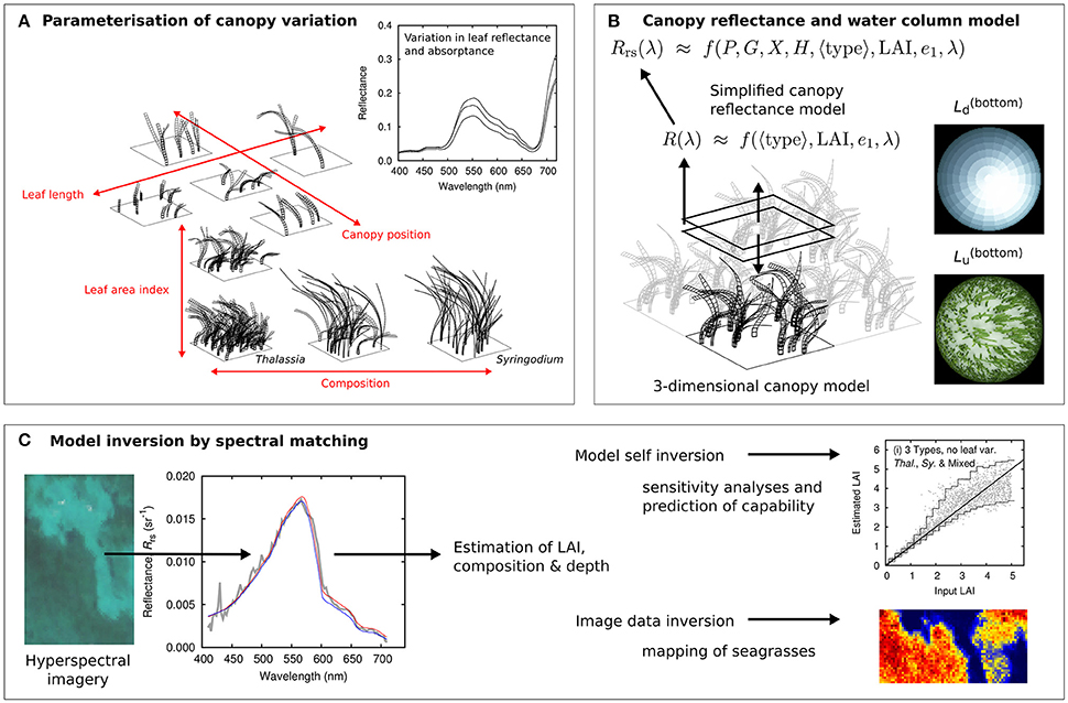
Figure 1. Overview of seagrass reflectance model and analysis. (A) Canopies are parameterized by four factors: Composition, leaf area index (LAI), leaf lengths, and leaf position. (B) A three dimensional canopy model estimates the top of canopy reflectance over all conditions and the results are reduced to a simpler functional form that includes the water column. (C) A spectral matching procedure applies the simplified model in sensitivity analyses and image processing.

Canopy Reflectance Model

The first step was to conduct many runs of a three-dimensional canopy model (Figure 1) for monospecific Thalassia, Syringodium, and 50:50 mixed canopies in terms of LAI, in order to establish the distribution of top of canopy spectral reflectance as a function of species, LAI, and canopy structure and position. Seagrass meadows are not monospecific in reality but often either Thalassia or Syringodium can represent greater than 70% of the total above-ground biomass of the macro-phyto-benthic community in Caribbean coastal habitats (Enríquez and Pantoja-Reyes, 2005). A range of community compositions are also common, associated with environmental conditions (Medina-Gómez et al., 2016). By including monospecific and 50:50 canopies in the model the idea was to cover the range of what might occur, with the concept of a mixed canopy included. The technical details of the model itself are described in Hedley (2008), Hedley and Enríquez (2010), and Hedley et al. (2014, 2015). Table 1 gives the full details of the treatments included in the model.

TABLE 1

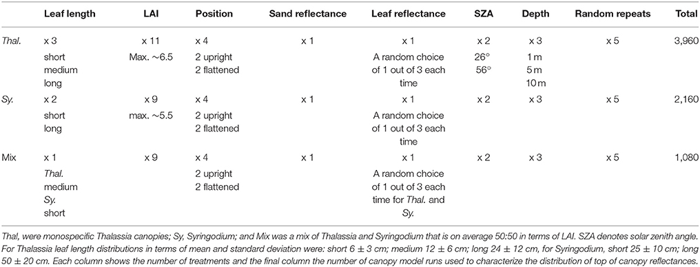
Table 1. Experimental design of model runs for establishing the variation of above canopy diffuse reflectance with LAI and other factors.

The factors of canopy structure and position were considered a source of variation, leaves were modeled as flexible strips that under simple model of wave motion assume naturalistic canopy positions, of which four treatments were used, two of each termed loosely “upright” and “flattened” (Table 1). The leaves are modeled as reflecting and transmitting surfaces 0.9 cm wide for Thalassia and 0.25 cm wide for Syringodium. In reality Syringodium leaves are circular in cross-section, however most previous modeling work and measurements of reflection and transmission treat Syringodium leaves in the same way as flat leaves (Thorhaug et al., 2007; Stoughton, 2009). The optical data to model them as circular volumes is not available and would be difficult to obtain in practical terms. The canopy model is also designed such that all leaves originate at the substrate whereas, unlike Thalassia, Syringodium has a short shoot from which leaves branch (Eiseman, 1980). Since the application here is remote sensing and not within-canopy light fields for photobiology (Hedley et al., 2014) these compromises are most likely optically insignificant in the context of the other factors such as canopy position (Figure 1), depth, and water column optical properties.

An important consideration was to incorporate variation in leaf optical properties, since the previous model (Hedley et al., 2015) assumed every Thalassia leaf had the same reflectance. In reality leaf reflectance varies at many scales: along the leaf length, between leaves and between sites (Hedley and Enríquez, 2010). Using only a single reflectance and absorptance spectra for all leaves represents an underestimate in that component of spectral variation, but how to quantify the appropriate variation at given spatial scale is not obvious. In this study each species was represented by three pairs of reflectance and absorptance spectra, corresponding to low, medium and high reflectance, coupled with high, medium, and low absorptance (Figure 2). The reflectance and absorptance data for Syringodium and Thalassia leaves were collected using samples of clean leaves from the Puerto Morelos reef lagoon, Yucatan, Mexico. Leaf reflectance spectra were measured using an Ocean Optics USB2000 spectroradiometer according to the methods described in Vásquez-Elizondo et al. (2017). Reflection, R_L(λ), was measured with a 2 mm diameter fiber optics placed over the surface of the sample at an angle of 45°C and a distance of 5 mm with a Teflon panel as a reference. Diffuse illumination was provided from light reflected from a semi-sphere coated with barium oxide (BaO) illuminated was with a white LED ring (450–650 nm) located around the sample, plus violet-blue LEDs and halogen lamps, to increase the diffuse illumination below 450 nm and above 650 nm (Vásquez-Elizondo et al., 2017). Transmission spectra were determined as T_L(λ) = 10^−D(λ), where D(λ) denotes absorbance, using a conventional spectrophotometer (AMINCO DW2, USA) controlled by an OLIS data collection system equipped with an opal-glass in front of the detector, following the methodology proposed by Shibata (1959) and described in Enríquez (2005) and Vásquez-Elizondo et al. (2017). Absorptance estimations were calculated as A_L(λ) = 1 − T_L(λ) − R_L(λ). For Syringodium, leaves were sampled from six sites and the three reflectance and absorptance pairs were selected from 193 optical determinations as representative of the range in the data. For Thalassia absorptance the model described in Hedley and Enríquez (2010) was used to generate spectral absorptance based on 50, 60, and 70% PAR absorptance, a typical range as shown in that paper. Additional reflectance measurements of leaf samples, not included in Hedley and Enríquez (2010) were taken to provide the three reflectance spectra (Figure 2A). For each individual modeled top of canopy reflectance (Table 1) one of the reflectance-absorptance pairs was selected for each species. This means that the spatial scale of the variation that is included was assumed pixel-to-pixel in a remote sensing context. This inclusion of variation in leaf reflectance is approximate, as the appropriate variation at a given spatial scale is unknown. However, to include no variation at all would be the weakest treatment because it could lead to spectral differences between the species for purely numerical reasons. Two spectra, as single data points, could have a distinguishing feature at random. Further discussion of these questions is deferred to the Discussion but the key point is that the specification of this variation (Figure 2) must be borne in mind when interpreting the results.

FIGURE 2

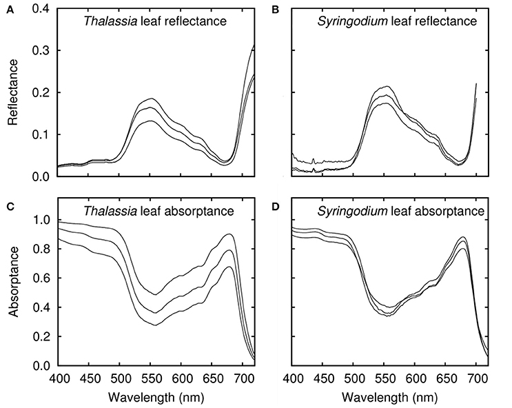
Figure 2. Leaf level reflectances and absorptances as used in the modeling for (A,C) Thalassia and (B,D) Syringodium. Each plot shows three lines, corresponding to the high, medium, and low reflectance variants (high reflectance being paired with low absorptance etc.).

The reflectance of the underlying sand was the same as that used in Hedley et al. (2015), being a typical calcium carbonate sand reflectance spectra with increasing reflectance in the red to a maximum of about 40% (Hedley et al., 2015). Note that in Hedley et al. (2015) the leaf reflectances were modified to include a component of sand reflectance to account for the observation that in some sparse Thalassia canopies there was sediment on the leaves, that term was not included here.

To factor in variations due to canopy BRDF (Bi-directional Reflectance Distribution Function) with repeat runs canopies were illuminated from two solar zenith angles, 26° and 56°, by sky radiance distributions computed by libRadtran, (Mayer and Kylling, 2005), and at three depths, 1, 5, 10 m, with the directional light field at depth computed by PlanarRad¹. These factors are discussed in more detail in Hedley et al. (2015). In the incorporation of the water column to the image analysis algorithm by necessity the top of canopy reflectance is considered Lambertian. Hedley et al. (2015) showed this simplification was insignificant in comparison to other factors but the propagation of the BRDF related uncertainty is retained for completeness.

The canopy model was configured to calculate in 16 spectral bands of 20 nm width over the range 400–720 nm and all reflectances were resampled to these bands. The spectral reflectance properties of Thalassia and Syringodium are dominated by chlorophyll a and b therefore no species-dependent fine scale spectral features are lost by this process (Figure 2).

Top of Water Column Reflectance Model

The next step was to develop a model of top of water column reflectance that was fast enough in application to be used for image analysis. For each of the three canopy species structures, mono specific Thalassia and Syringodium and the 50:50 mix, the reflectance at each wavelength was fitted to an exponential model of the form,

$\begin{array}{cc}R\left(\lambda \right)=A\left(\lambda \right)\text{exp}\left[-k\left(\lambda \right)\times \text{LAI}\right]+B\left(\lambda \right)+\epsilon \left(\lambda \right)& (1)\end{array}$

Where the A(λ), k(λ), and B(λ) values were deduced by regression over all the canopy model results for each canopy type. An exponential decrease in reflectance with LAI was shown to work well in the previous study (Hedley et al., 2015). The term ε(λ) represents a set of spectra, which are the residual differences between the regression model and the actual spectra, largely due to the factors that introduce variation. It is assumed that ε(λ) can be treated as random since we are not interested to deduce factors such as canopy position. A model for the range of magnitude and shape of ε(λ) is established by principle components analysis and ε(λ) is reduced to a wavelength independent single parameter e₁, which ranges from 0 to 1 (Hedley et al., 2015). A check is performed that the full model, including the component captured by e₁ can replicate all the top of canopy spectra to within acceptable accuracy (Figure 3). On this basis one error term was judged sufficient, so top of canopy spectral reflectance becomes a function of species composition (canopy type), leaf area index, and the random error term drawn from a uniform distribution of 0 to 1.

$\begin{array}{cc}R\left(\lambda \right)\approx f\left(\langle type\rangle ,\text{LAI},e_1,\lambda \right)& (2)\end{array}$

FIGURE 3

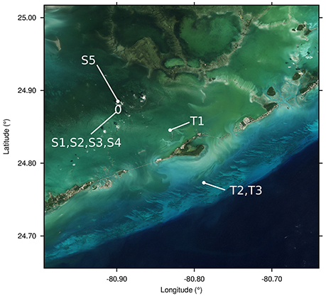
Figure 3. The five Syringodium dominated locations (S1-S5) and three Thalassia dominated locations (T1-T3) where the in situ LAI and depth data points were located. Image produced using Sentinel-2A data from the European Space Agency.

This expression was embedded into Lee et al.'s (1998, 1999) semi-analytical model for shallow water remote sensing. A input parameter of Lee et al.'s model is bottom spectral reflectance, R(λ), so using Equation (2) this input can be eliminated and a function of the following form implemented,

$\begin{array}{cc}{R}_{\text{rs}}\left(\lambda \right)\approx f\left(P,G,X,H,\langle type\rangle ,\text{LAI},e_1,\lambda \right)& (3)\end{array}$

where the remote sensing reflectance, Rrs(λ), at wavelength λ is calculated dependent on the amount of phytoplankton (P), dissolved organic matter (G), backscatter (X), depth (H), and bottom reflectance R(λ). LAI, < type>, and e₁ represent the canopy, where < type> is a categorical parameter (integer) taking the value 0, 1, or 2 for Thalassia, Syringodium, or mixed canopy type respectively. This model can be used in both forward mode, to estimate the remote sensing reflectance for a specific situation represented by the input parameters, or in inverse mode using a successive approximation technique such as Levenberg-Marquardt (Wolfe, 1978), where the input parameters that give the best least-squares match to a given remote sensing reflectance are deduced. Since <type> in Equation (3) is not a continuous parameter, for inversion three best-fit solutions are found for <type> = 0, 1, 2, and the overall best fit is considered the optimal solution and determines canopy composition type. The possible range of the parameter values for all inversions in this study were P [0, 0.2]; G [0, 0.5]; X [0, 0.05]; H [0, 20]; LAI [0, 6]; e₁[0, 1] (Table 2). The possible canopy type was in some cases restricted, or all three of Thalassia, Syringodium, or 50:50 mix were used. For further details of what underlies Equation (3) see Hedley et al. (2009, 2015).

TABLE 2

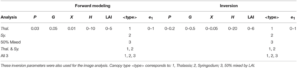
Table 2. Sensitivity analysis design showing range of parameters used for forward modeling and for inversion.

In the sensitivity and image analyses, Equation (3) was evaluated at a wavelength resolution corresponding to a subset of the bands of the PRISM hyperspectral data, specifically 107 bands with centers from 410 to 710 nm. The canopy model results and other spectrally tabulated coefficient data were resampled to these wavelengths by linear interpolation. Local optima in the inversion were avoided by repeating each inversion five times with a random parameter start point, and the best matching solution of the five taken.

Sensitivity Analysis

The model for remote sensing reflectance (Equation 3) was applied in a sensitivity analysis to deduce the fundamental uncertainty, which occurs when two different physical situations lead to the same remote sensing reflectance within a tolerance that is negligible in practical terms. In other words, spectra are so close that they cannot be reliably differentiated. The model included sources of variation in spectra from components of the system up to the top of the water column, with the intention that it would be applied to atmospheric and glint corrected imagery. Optical processes that occur above the water column that cause pixel-to-pixel variation were outside the scope of the model and are effectively noise. In this context the fundamental uncertainty can be deduced by noise perturbed self-inversion of the model. i.e., a specific set of parameters are used to model remote sensing reflectance from Equation (3), a random noise term is added on, then the model is inverted to see if the input parameters can be recovered. The variability in the recovered parameters is the fundamental uncertainty of the model in the context of the noise. In the sensitivity analysis we used a spectrally correlated noise model (Hedley et al., 2012a; Garcia et al., 2014) based on the covariance matrix over a deep water area of the Florida Bay PRISM imagery (see next section). Being empirically derived, the covariance matrix captures all sources of pixel to pixel variation that occur over the deep water area, including both environmental effects and instrument noise. A spectrally correlated model is used because a large part of the noise is residual surface glint, even after images have been glint corrected (Kay et al., 2009), and so is not independently random in each band.

The model of Equation (3) was used to randomly generate spectral remote sensing reflectances with parameters being drawn from uniform distributions over the ranges in Table 2. Depth ranged from 0 to 10 m, LAI from 0 to 5. Five separate analyses were conducted, three where canopy type was fixed as only one of the basic classes: Thalassia, Syringodium, or a 50:50 mixture, one where canopy type could be one of either Thalassia and Syringodium, and one where each modeled spectra could arise from any of the three classes. The idea was to simulate varying degrees of canopy composition changes from pixel to pixel, and investigate the consequences of introducing canopy type variability. All five analyses were performed three times: (1) using results with leaf level reflectance variation (Figure 2); (2) using only canopies modeled with no leaf level variation in reflectance and absorptance: using the medium reflectance and absorptance (middle lines in Figure 2); and (3) using the canopy reflectances directly from the 3D canopy model, hence bypassing the simplified reflectance model (Equation 1) and using more “realistic” canopy reflectances in the forward model while retaining the simplified model in the inversion. The aim was to understand the consequences of introducing leaf level variation to the fundamental uncertainty, and also to verify if the performance of the simplified canopy model against the 3D canopy model which it is based. For the forward modeling the water optical properties were fixed at the values shown in Table 2. This is equivalent to assuming an area of spatially homogenous water optical properties.

For each analysis, 15 in all, 2,500 random spectra were generated by the forward model, random noise was added on and then the inversion model was applied to attempt to recover the input parameters. The resulting dataset facilitated an investigation into the various sensitivities of the model and is presented in the Results and Discussion section.

Image Data Analysis

The inversion model was applied to hyperspectral airborne imagery acquired by the Portable Remote Imaging Spectrometer (PRISM) instrument (Mouroulis et al., 2014) in Florida Bay, January 2014 (Dierssen et al., 2015), using 107 of the PRISM bands from 410 to 710 nm. Details of the imagery pre-processing are given in Hedley et al. (2015), but in short this consisted of: atmospheric correction and conversion to R_rs(λ) using a modified version of the ATREM radiative transfer model (Gao and Davis, 1997); per-pixel sun-glint correction by use of the Rayleigh-corrected reflectance at 980 nm; and a vicarious calibration adjustment based on above-water spectral reflectance measurements taken with an ASD FieldSpec 4 co-incidentally with image acquisition (Dierssen et al., 2010). The imagery is at ~1 m resolution. The above-surface solar zenith angle was ~30° at the time of acquisition.

A number of flight lines were available, some of which covered sites at which canopy composition, LAI, and depth had been recorded co-incident with GPS data (see Hedley et al., 2015 for methods). The data included areas that were dominated by Thalassia or Syringodium, typically located ocean side or bay side respectively (Figure 3). The analysis utilized eight locations from three flight lines that covered the in-situ data locations, and varied in pixel size from ~1 to 2 m. Five locations (S1-S5) were Syringodium dominated (close to monospecific) and three (T1-T3) where Thalassia dominated. Each location contained between two and 12 in-situ data points of LAI determinations based on 20 × 20 cm quadrats in transects spaced 2 m apart. In total 42 data points were available however the seagrass beds were patchy and in some cases visual inspection indicated that the location of the data in the imagery was only reliable to within a few meters. For this reason precise image to data registration of the 42 individual points was not possible and the data was processed as grouped into the eight locations. At each location the mean and standard deviation of LAI estimates from 4-pixel window (~4–8 m dependent on pixel size) around the data points was taken, and compared to the mean and standard deviation of the in-situ data points at that location. Depth data was also available for each of the eight locations; this was assumed constant at each location.

Parameterization of the model for image processing was the same as described in the sensitivity analysis, inversion ranges as in Table 2 and with all three bottom composition types included. A deep water area at the end of the flight line containing the Thalassia dominated canopies was used to characterize the above-surface noise covariance matrix (the same noise matrix as used in the sensitivity analysis), the other flight line did not have a suitable deep water area for noise assessment, so the same above surface noise was assumed. For each pixel 20 noise perturbed inversions were performed to provide the mean results and 90% confidence intervals for the parameters of interest, in particular LAI and depth.

Results and Discussion

Variation in Modeled Top of Canopy Reflectance

The leaf level reflectance measurements of Thalassia and Syringodium (Figure 2) were consistent with those measured by others for those species and for other seagrasses (Lüning and Dring, 1985; Zimmerman, 2003; Runcie and Durako, 2004; Enríquez, 2005; Thorhaug et al., 2007; Stoughton, 2009) although our reflectances tended to be higher at the peak of 550 nm. Consistent with Enríquez (2005) and Thorhaug et al. (2007) the spectral shapes of the leaf reflectance of Thalassia and Syringodium were almost identical to each other and the reflectance of Syringodium at 550 nm was slightly higher than Thalassia (Figure 2).

The first question of interest in this study is how the sources of variation in the 3D canopy model affected the top of canopy reflectances for Thalassia and Syringodium, and in particular the relative contribution of variation of leaf level reflectance. The input data on reflectance and absorptance of Thalassia and Syringodium leaves contains a wider variation for Thalassia than Syringodium, especially in terms of absorptance (Figure 2). This has a consequence for the variation in the top of canopy reflectance (Figure 4). For Thalassia at an LAI of 3 the variation in reflectance at 630 nm was around three times greater when leaf level variation is included (Figure 4B vs. Figure 4A), whereas for Syringodium the variation in reflectance was relatively unaffected by the introduction of leaf level variance (Figure 4D vs. Figure 4C). At a given LAI the “base level” variation induced by variation in canopy structure and position was similar for Thalassia and Syringodium (Figures 4A,C); a small level of variation in leaf optical properties is negligible in comparison (Figure 4D) but clearly above a certain threshold of leaf level variation the variation in canopy reflectance becomes much greater (Figure 4C). In our data Syringodium was below this threshold and Thalassia was above it. Whether this level of variation is appropriate for the spatial scale of the remote sensing analysis (1–2 m pixels) remains unknown, as the data were not collected with this objective in mind, this will be discussed later.

FIGURE 4

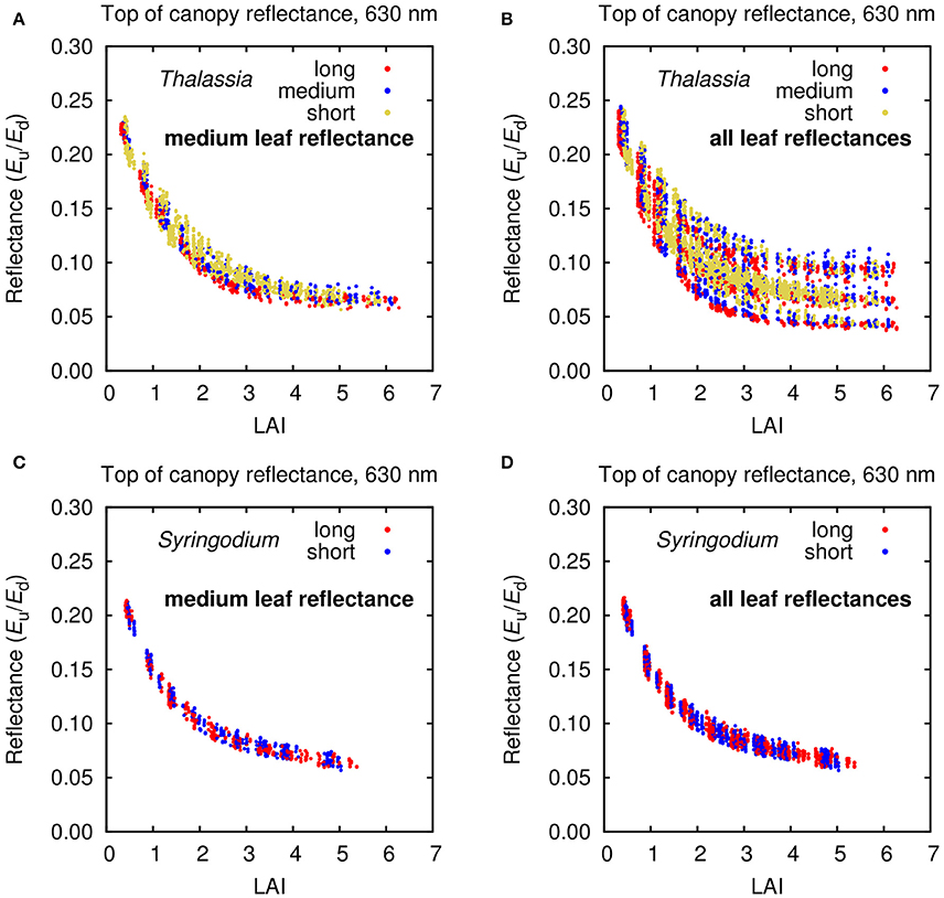
Figure 4. Top of canopy (TOC) reflectance at 630 nm for modeled (A,B) Thalassia and (C,D) Syringodium canopies under all treatments but differentiated by (A,C) medium leaf reflectances only and (B,D) all three leaf reflectance and absorptance treatments.

Spectral Separability in Top of Canopy Reflectance

Given the level of variation introduced by canopy position, structure, and leaf level variations (Figure 4) the next question is how much spectral separability for determining LAI or between canopy compositions of Thalassia and Syringodium remained in the top of canopy reflectances? While this will be answered more comprehensively by the sensitivity analysis an initial band ratio plot for 450 and 550 nm for all of the modeled canopy reflectances indicates that separability in the model data is possible (Figure 5). Considering LAI first (Figure 5B) there was a clear trend of darkening in both bands where LAI graduates across the plot area. Despite a few isolated places where, for example, LAIs of 5 were mixed with LAIs of 3, there is a monotonic trend in LAI in both bands up to LAIs of around 4. This is consistent with the previous Thalassia only model (Hedley et al., 2015) and suggests the introduction of Syringodium does not compromise this capability.

FIGURE 5

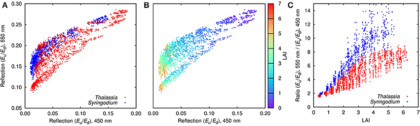
Figure 5. Distribution of top of canopy (TOC) reflectance for all modeled Thalassia and Syringodium canopies with 26° solar zenith angle, in two band space: 450 and 550 nm. (A) Distribution by species, (B) distribution color coded by LAI, (C) band ratio of reflectance at 550–450 nm, as a function of LAI. Note that all points are plotted in a random order so the dominance of a color in particular area does not arise simply because other points are obscured.

The ability to spectrally discriminate species in the modeled top of canopy reflectances is less clear (Figure 5A). Syringodium was distributed in the upper range of the variation with respect to reflectance at 550 nm, in part at least because leaf reflectance was generally higher at 550 nm (Figure 2), but still overlaps with Thalassia in the two-band space of 450 and 550 nm. At any specific LAI the species were separable by the ratio of reflectance at 550–450 nm (Figure 5C), but for ratio values less than around eight either species could be present but with different LAIs. There is a region on the left of Figure 5A where only Syringodium occurs, corresponding to an LAI greater than 3 (c.f. Figure 5B), this corresponds to reflectance ratios greater than 8, where only Syringodium occurs in Figure 5C. In this region Syringodium could be distinguished from Thalassia in top of canopy reflectance using only the bands at 450 and 550 nm. The basis of this is that in our data at 550 nm Syringodium leaves were slightly brighter than Thalassia to an extent that is beyond the incorporated variation, but at 450 nm they were similar. Capability for discrimination using all the spectral bands can only be greater, but water column variations and above surface noise will compromise that ability.

Simplified Model for Top of Canopy Reflectance

The next set of results verified that the simplified model for top of canopy reflectance (Equation 1) for each canopy composition adequately captured the variations previously discussed. The question is how much is “lost” going from the 3D model reflectances to the simplification of Equation (1). This is also checked later in the sensitivity analysis, but the first evaluation is to consider the magnitude of the residual spectra between the 3D canopy model reflectances and those that can be produced by the simplified model (Figure 6). In all cases the spread of the residuals was very small compared to the range of reflectances captured. For wavelengths lower than 700 nm, over all six models 70% of the 90% confidence intervals on the residuals were less than 5% of the reflectance range, and nowhere were the residual 90% confidence intervals greater than 10% of the reflectance range. Residual ranges greater than 5% of the reflectance only occur when leaf level optical variation is introduced. This indicates that leaf level optical variation does introduce different modes of variation that can't be captured by a single variation term (e₁, section Top of Water Column Reflectance Model). But since the effect is small a single error term was retained for this study.

FIGURE 6

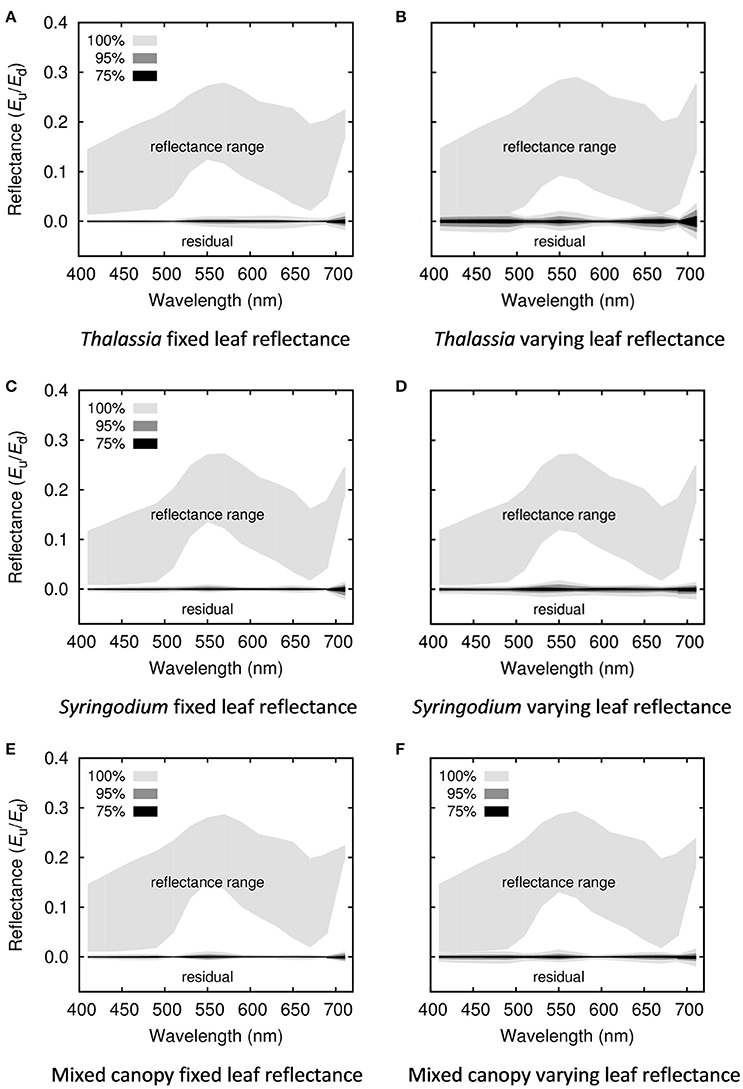
Figure 6. Magnitude of discarded residuals for each of the simplified canopy models for (A,B) Thalassia, (C,D) Syringodium, (E,F) 50% mixed canopies of Thalassia and Syringodium, and for (A,C,E) canopies where leaf reflectance is fixed, (B,D,F) variable leaf reflectance. The upper region of each plot shows the full range of reflectances from all treatments in the 3D canopy model, the lower line shows the magnitude of the discarded residual error when the model is simplified, in terms of 100, 95, and 75% of the inputs, i.e., 75% of the residuals lie with the bounds of the 75% shaded region.

Sensitivity Analysis—Bathymetry

The sensitivity analysis indicated that the fundamental uncertainty for bathymetry was very low under all treatments (Figure 7). Even for the treatment that included the most sources of variation, including all three canopy compositions of Thalassia, Syringodium, and 50% mixtures, 90% confidence intervals on bathymetry retrieval were better than ±1 m at 10 m depth (Figure 7J). For the other treatments the confidence intervals on bathymetry retrieval mirrored the amount of variation included in the model; the confidence intervals for canopy treatments of single composition types with no leaf level variation were particularly narrow (Figures 7A,C,E). That bathymetry is a robust result under physics based inversion approaches is well-established (Dekker et al., 2011) and this result is as expected. What is important here is that introducing different canopy compositions and leaf level optical variation made very little difference to the fundamental uncertainty in bathymetry. However, being an estimate of the uncertainty from self-inversion of the model this is an upper bound on what could be expected in a real application. The possibility of errors in image pre-processing is neglected, for example.

FIGURE 7

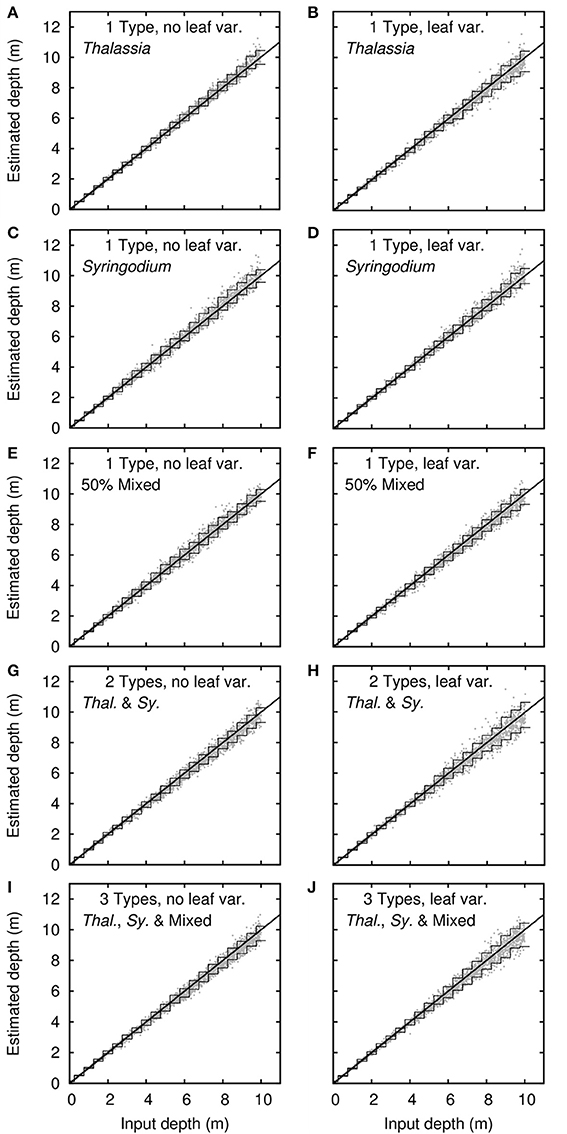
Figure 7. Sensitivity analysis results for bathymetry. Dots are 2,500 noise-perturbed self-inversion results, lines are mean 90% confidence intervals binned in steps of 0.5 m. Treatments are (A–F) single benthic types of Thalassia, Syringodium and 50% mixed canopies, plus (G–J) models with multiple bottom types. Right and left columns are with and without variation in leaf reflectance.

Sensitivity Analysis—Leaf Area Index

Leaf area index was a less robust result than bathymetry (Figure 8). The confidence intervals for LAI retrieval are relatively large, especially for LAIs greater than 2. This corresponds to the increasing saturation of the LAI effect on reflectance as canopy reflectance becomes less, beyond a certain LAI no further darkening can occur and approaching this limit uncertainties become high (Figure 5) (Knyazikhin et al., 1998). In the inversion parameter limits (Table 2) the upper limit on the LAI confidence interval is capped at 6 and this explains why the upper confidence interval curves toward the horizontal for high LAIs (Figure 8). The upper limit acts to reduce the uncertainty and is akin to including the a priori information that LAIs greater than 6 cannot occur. Including a priori limits or probabilities is useful for reducing uncertainty in inversion methods (Jay and Guillaume, 2016) but is unsuitable if anomalies are of interest or the bounds are too restrictive. Other seagrass species such as Posidonia sinuosa and Posidonia oceanica can achieve much higher LAIs (e.g., >8 reported in Collier et al., 2007; and >12 reported in Olesen et al., 2002, respectively) and in that case it would be preferable that the uncertainty accurately reflects this.

FIGURE 8

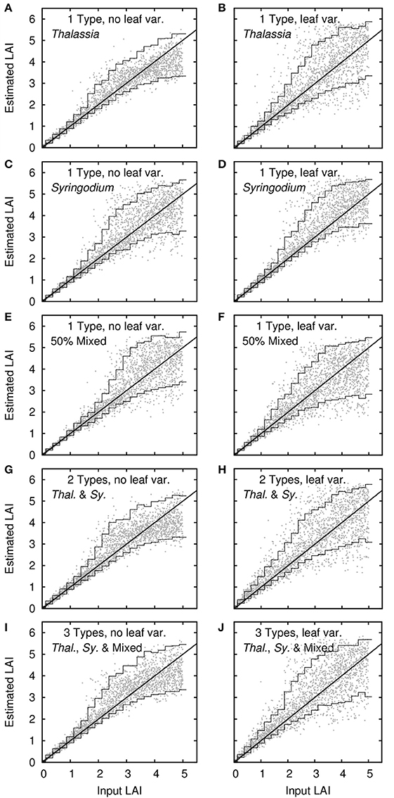
Figure 8. Sensitivity analysis results for leaf area index (LAI). Dots are 2,500 noise-perturbed self-inversion results, lines are mean 90% confidence intervals binned in steps of 0.25 in LAI. Treatments are (A–F) single benthic types of Thalassia, Syringodium and 50% mixed canopies, plus (G–J) models with multiple bottom types. Right and left columns are with and without variation in leaf reflectance.

Leaf area index was also more sensitive to the specific canopy composition treatment or inclusion of leaf level variation, but not exceptionally so and without any clear pattern (Figure 8). Introducing leaf level optical variation in general increased uncertainty in LAI retrievals, as expected, but the effect was relatively small. Interestingly, without leaf level variation Syringodium LAI determinations had higher uncertainty than for Thalassia (Figure 8C vs. Figure 8A). This was likely the result canopy position and structure, the longer and thinner leaves of Syringodium will have a greater effect on the apparent areal density as viewed from above, when they assume different positions. The higher leaf level variation in Thalassia (Figure 2) more than compensated for this factor and when leaf level variation was included Thalassia had slighter higher uncertainty (Figures 8B,D). Overall though, all treatments performed similarly, and introducing a model with two species (Figures 8G,H) or two species plus mixtures (Figures 8I,J) did not greatly increase the uncertainty in LAI estimation.

Sensitivity Analysis—Canopy Composition

Determining the canopy composition type, either monospecific Thalassia or Syringodium, or between the two monospecific canopies and 50:50 mixed canopies, would be expected to have high uncertainty since the spectral shapes of Thalassia and Syringodium leaf optical properties are almost identical (Figure 2, and Thorhaug et al., 2007). However, as previously mentioned, in our model a degree of species separability at the top of canopy exists because the Syringodium was relatively brighter than Thalassia at 550 nm (Figure 2). The sensitivity analysis also indicates some capability for species discrimination, in fact for depths less than 0.5 m the self-inversion analysis was able to accurately recover the canopy composition type 100% of the time (Figure 9), hence even including low LAI conditions that Figure 5 indicated might be inseparable. Therefore, despite including above surface noise, the top of canopy reflectances were spectrally separable to a much greater extent than implied by the two-band analysis of Figure 5. This is partly a consequence of the simplified canopy reflectance model, which reduces variation by multiple factors into a single degree of freedom. However, this issue is not large, when using the original 3D canopy model reflectances in the forward model, accuracy in composition type for depths less than 0.5 m is in the range 60–80% for most treatments (Figure 9), but by a depth of 4 m the ability to distinguish canopy type has reduced to around 50–70% and any artefactual advantage in using the simplified canopy forward model is lost. This provides an alternative estimate of the “cost” of the simplified canopy model: At a depth of 4 meters the above surface noise in relation to the benthic “signal” was already greater than what was lost in simplifying the canopy model.

FIGURE 9

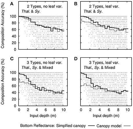
Figure 9. Sensitivity analysis results for the accuracy of canopy composition type determination as function of depth. Each dot is the overall accuracy from the uncertainty propagation (20 repeats) of each of the 2,500 noise-perturbed self-inversions. Dark lines are the mean accuracy binned in steps of 0.5 m. Thin lines are the mean accuracy when input bottom reflectances are drawn directly from the canopy model results. Treatments include (A,B) the model of two bottom types and (C,D) three bottom types. Each is repeated (B,D) with and (A,C) without leaf level variance.

Ability to determine canopy composition decreases with increasing depth (Figure 9). For canopies that can be either Thalassia or Syringodium (Figures 9A,B) a random choice would be correct 50% of the time, so at 10 m depth separability of ~60% indicates the ability to determine species is almost completely lost. Likewise for three bottom compositions of Thalassia, Syringodium, or mixed canopies ~40% accuracy at 10 m is close to a random choice.

It might be expected that the ability to determine species would increase with LAI, since the “signal” of the species would be expected to increase with leaf area. This was true only for treatments that included leaf level optical variation, and the effect was small (Figures 10B,D). For multiple canopy types where there was no leaf variation, ability to discriminate canopy composition actually decreased slightly with LAI (Figures 10A,C). However, these results do not give any strong indication since overall ability to discriminate canopy type was averaged over all depths from 0 to 10 m, the primary conclusion is depth was the more significant factor (Figure 9).

FIGURE 10

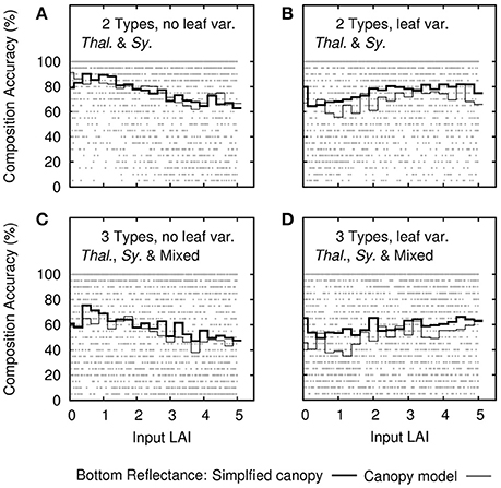
Figure 10. Sensitivity analysis results for the accuracy of canopy composition type determination as function of leaf area index (LAI). Each dot is the overall accuracy from the uncertainty propagation (20 repeats) of each of the 2,500 noise-perturbed self-inversions. Dark lines are the mean accuracy binned in steps of 0.25 in LAI. Thin lines are the mean accuracy when input bottom reflectances are drawn directly from the canopy model results. Treatments include (A,B) the model of two bottom types and (C,D) three bottom types. Each is repeated (B,D) with and (A,C) without leaf level variance.

The sensitivity analysis is therefore pessimistic as regards the ability to distinguish between Thalassia and Syringodium by remote sensing. These results should be considered upper bounds of what is achievable, in the context of what is included in the model. That is, in any application results can only be worse unless there is some aspect not included in the model that could be leveraged to facilitate species discrimination. In Florida Bay Syringodium tends to occur bay-side whereas Thalassia is ocean-side, therefore there could be systematic differences in water optical properties co-incident with species that would increase discrimination. Here, we have only considered clean leaves free of large epiphytes. Thalassia leaves have a longer life span than Syringodium, which facilitates the formation of more complex epiphyte communities on the leaves. The dominant epiphyte taxa are calcifying red coralline algae, although foraminifera, diatoms, and other small calcifiers have also been reported (Corlett and Jones, 2007). Epiphyte cover is greatest at the apical segments of Thalassia leaves, since these are the oldest part of the leaf. Being located at the top of the canopy there is good potential for epiphytes to contribute to the reflectance. On the other hand, red wavelengths, where coralline algae are spectrally distinct, have low penetration in water so any discrimination advantage may be limited to the shallowest canopies. The situation will also vary between canopies since dependent on conditions some canopies are relatively free of epiphytes and the epiphyte community follows a progressive process of organization coupled with leaf age (Cebrián et al., 1999), Understanding the epiphyte contribution for the purposes of optical modeling is therefore a complicated task, but these kind of co-incident factors could explain the relatively reasonable performance of classification techniques applied to multispectral data (Phinn et al., 2008).

Image Data Analysis

Visually, LAI results from the hyperspectral imagery appeared reasonable over both the Thalassia and Syringodium dominated areas (Figure 11). Sand areas were identified as LAI close to zero, and denser seagrass areas, especially over Syringodium dominated locations, contained the full range of LAIs up to 5 or more, which was the limit of discrimination predicted by the sensitivity analysis (Figure 8). The algorithm output did highlight some artifacts in the source imagery such as a vertical line (Figure 11, left LAI image) presumably corresponding to detector anomaly such as dust contamination. Image-derived LAI corresponded well to in situ data in terms of both area-averaged LAI and standard deviation at each location (Figure 12A). Linear regression of the area-averaged estimated LAIs against the in situ data yielded an r² of only 0.32 with a y-intercept of 1.54 and slope of 0.48 (Figure 12B). However, it is clear that the method identifies areas of zero LAI very well (Figure 11) but there is no in situ data at zero LAI to represent this. Acknowledging this capability by constraining the regression to have an intercept at zero gives an r² of 0.86 and a slope of 1.01 (Figure 12B). This would seem a more sensible result given visual interpretation of Figure 11: zero LAI areas are not identifed as LAI of 1.54. In general the high variation exhibited by the in situ LAI point data at a scale of 2 m (the transect sampling distance at each location) is clearly a confounding factor for validation of a remote sensing analysis. It places a very high demand on the geo-correction of the imagery and accuracy of the GPS system. The in situ data used here was not collected with this study in mind, for future studies placing benthic markers that can be identified in the imagery may be a better solution (Mumby et al., 2004). Nevertheless, both visually and in comparison to the available data (Figures 11, 12) LAI estimations from the image data analysis appear reasonably accurate.

FIGURE 11

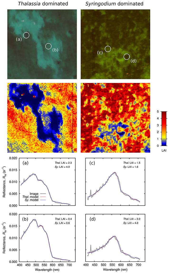
Figure 11. Application of inversion model to hyperspectral PRISM imagery in (left) a Thalassia dominated area (T2 and T3) and (right) a Syringodium dominated area (S1). LAI image is from model containing all bottom compositions, (a–d) show spectral matches for models constrained to Thalassia or Syringodium only.

FIGURE 12

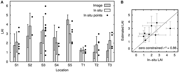
Figure 12. (A) Leaf area index as estimated from imagery compared to in-situ data, for the five sites dominated by Syringodium (S1-S5) and the three by Thalassia (T1-T3). Bars show mean and standard deviation for in-situ data points and for a 4-pixel window around those points. The number of pixels contributing to each bar varies from 71 to 170. The individual data points at each location are plotted to show the variation that exists at each location. (B) Scatterplot of LAIs from in-situ data and 4-pixel window imagery estimates, i.e., the same information as in the bars in (A).

Depths at the eight locations ranged from ~1.5 m to 8 m, depth estimates from the inversion model agreed well in general but there was a dependency on LAI (Figure 13). All locations except T1 were highly heterogeneous in terms of canopy density, to generate Figure 13 the mean estimated depth at 5 pixels with relatively low LAI within an approximate 20 m radius were taken, and likewise depth estimates from pixels with relatively high LAI within that area. Figure 13 therefore gives an indication of the effect of LAI on depth estimation at each location. A regression plot using both low and high LAI results (Figure 13B) gave an r² of 0.94 and slope of 1.10. Clearly this is a good result but the number of data points is too low to make any strong conclusions. It might be expected that high LAI, giving rise to darker pixels, would cause depth over-estimation. Indeed for most cases over low LAI areas (typically bare sand) depth estimates were quite accurate while for high LAI depth was over-estimated (Figure 13A, S1, S4, T2, T3, and Figure 13B). However, the pattern was not always consistent, in fact the highest LAI areas (S2, S3, LAI greater than 5) gave good depth estimates. It seems that intermediate LAIs give rise to the largest potential for depth over-estimation. The largest depth errors were greater than the uncertainty in depth estimation predicted by the sensitivity analysis over all LAIs (Figure 7J) and the uncertainty propagation (error bars in Figure 13). The sensitivity analysis of Figure 7 covers LAIs from 0 to 5, but if the analysis is restricted to LAIs from 3 to 4 the plots appear almost identical and the depth uncertainty is still only around ±1 m at 10 m depth. In comparison at S1 an LAI of 3 gave rise to error of +1.5 m in a depth of 2.4 m. The true depth at location S1 lies outside the uncertainty estimates for the high LAI pixels and so points to either an omission from the model or a radiometric discrepancy between the model and the image data. In other words, the spectral reflectance from the image data does not lie within the possibilities that can be produced for a depth of 2.4 m from the forward model. It is worth noting that the parameters for the optical properties of the water column, P, G, and X, are not estimated as their minimal or maximal values (Table 2) and so are not unduly constraining the inversion.

FIGURE 13

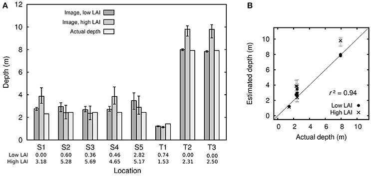
Figure 13. (A) Depth estimates for the five sites dominated by Syringodium (S1-S5) and the three by Thalassia (T1-T3). Low LAI and high LAI are each averages over 5 pixels within an approximate 20 m radius of the location center, selected as examples of low and high LAI pixels. Error bars are the mean of the upper and lower 90% confidence intervals from the uncertainty propagation. (B) Scatterplot of actual depth against estimated depths over low and high LAI locations, i.e. the same data as (A).

With respect to canopy composition, model inversion uniformly converged on a solution for monospecific Thalassia canopies. Even over the Syringodium dominated sites (Figure 11, right, S1) the model almost never selected Syringodium canopies or a 50:50 mix as giving the best spectral match. The only exceptions occurred on or around the edges of sand patches where LAI was close to zero so canopy composition is irrelevant. The sensitivity analysis suggested that discrimination of species would be subject to high uncertainty (Figure 9), but that one bottom type is systematically chosen in all cases indicates an issue of the radiometric alignment of the model with the image pixel reflectances, since the expected outcome under high uncertainty would be random bottom composition.

Sensitivity Analysis vs. Image Data Results

While overall the results for LAI and depth are reasonable, a few discrepancies have arisen between the performance predicted by the sensitivity analysis and the performance demonstrated by application to image data. The sensitivity analysis and uncertainty propagation are based on the assumption that the forward model is (1) radiometrically aligned with the image reflectances, i.e., ideally both the model is accurate and the image data is radiometrically accurate, or at least they are systematically comparable; and (2) that the model incorporates all possible sources of variation that could occur over the application area. If either condition is not met, then the behavior when applying the model to the image data will lead to results outside the scope of the sensitivity analysis.

The spectral matches achieved were in general very good (Figures 11a–d). Over either the Thalassia or Syringodium dominated sites when the model was constrained to only allow one composition type, then either Thalassia or Syringodium canopies were capable of generating spectra that matched the overall shape of the image reflectances, and which were virtually indistinguishable from each other (Figures 11a–d). It is therefore not surprising Thalassia and Syringodium could not be discriminated in the image data, any spectral difference in the forward model due to canopy composition was negligible in comparison to the residual fit between the model and image data. One reason that the Thalassia composition is preferentially selected may be that the Thalassia canopy model contains more leaf level optical variation that does Syringodium (Figure 2) so the greater degree of freedom permits a marginally closer match than is possible with the Syringodium model. This implies that incorporating uncertainty could bias the inversion when the model and reflectances aren't exactly radiometrically aligned, and this may be a limitation of the approach. How much variation is the correct amount to include in the canopy modeling is also difficult to assess. Strictly it should be the pixel-to-pixel variation at the scale of image pixels within the spatial domain of the application, but to quantify this is unrealistic. A better approach may be to standardize the amount of optical variation between species, as this might remove the bias or at least reveal the extent by which the inversion was biased by differences in uncertainty.

The spectral matches from the model at the Syringodium dominated site S1 (Figures 11c,d) do not fully capture the chlorophyll absorption features in wavelengths from 570 nm upward (Jeffery et al., 1997). The model is a smoother approximation because the 3D canopy model operates at 20 nm resolution. Improving the spectral resolution of the canopy model may help match these chlorophyll features and disambiguate increased LAI from increased depth, although that issue primarily afflicted the deeper site where these features are almost absent in the image data (Figures 11a,b). These spectral features are unlikely to assist in species discrimination since they are also present in reflectances from the shallow Thalassia site (T3, data not shown). In particular the shoulder at 570 to 585 nm and reflectance peaks at ~645 nm and ~690 are ubiquitous and arise from features also visible in the leaf level reflectances for both species (Figure 2).

The flight line over the Syringodium site S1 (Figures 11c,d) contained much more spectral noise up to 550 nm than for the Thalassia sites (Figures 11a,b). However, the band-to-band noise appears to average out satisfactorily with respect to the overall spectral fit. The documented signal to noise ratio of the PRISM instrument is more than adequate for this application. By the sensitivity analysis parameterization (Table 2) the reflectance change at 550 nm to detect 1 m change in depth at a depth of 10 m over a canopy of LAI 4 is 0.8% of the reflectance for bare sand at zero depth (the brightest target required for subsurface applications). This dynamic range would be covered by a signal to noise ratio (SNR) of 120 and 8-bit digitization, while PRISM is 14-bit with an SNR of 200 per band, and much greater when bands are combined as they are here (since fitting a spectrum is a effectively a kind of band-averaging) (Mouroulis et al., 2014). So for hyperspectral imagers such as PRISM the radiometric limiting factors, especially for physics based aquatic applications, lie not in the instrument specifications but in the data processing (see also Goodman et al., 2008; Hedley et al., 2012b). Since here discrepancies between the sensitivity analyses and practical performance appear to be due to radiometric differences between the model and data, this suggests future model based sensitivity analyses should include a term for “radiometric discrepancy.” That is, regardless of the cause of such a discrepancy (atmospheric correction issues, model inadequacy, etc.) it seems overly optimistic that such a term should be zero. The common practice of relying entirely on a sensor or environmental noise characterization (Brando et al., 2009; Hedley et al., 2012b, 2015; Garcia et al., 2014) is not really adequate to predict practical performance.

Implications for Remote Sensing of Seagrasses

In this study, the sensitivity analysis suggested the ability to discriminate between T. testudinium and S. filiforme by remote sensing is at best weak. In a practical application reflectance spectra arising from either canopy were virtually identical, with differences below the accuracy of the radiometric alignment of the model with imagery data. The situation with respect to other species may be better, Fyfe (2003) indicated that Zostera capricorni, Posidonia australis, and Halophila ovalis were separable in terms of leaf reflectance, but that study did not include other sources of variability at remote sensing scales. For those species spectral matching may be more effective if the matching were weighted on wavelength regions in which discrimination is possible, but this would be at the cost of other factors such as depth determination.

On the other hand, a physics-based approach with spectral matching may not be the best way to extract species information. Phinn et al. (2008) demonstrated a weak ability to map seagrass species using a classification approach on 54-band CASI data (Compact Airborne Spectrographic Imager). Of eight classes of canopy composition (including five species) around three classes were identified with overall accuracies greater than around 40%. However, the classification applied in Phinn et al. (2008) was based on top of water column reflectances, so if for example species were associated with depth then the classification can use this information since it is also contained in the reflectance spectra. Classification approaches are in general able to use whatever information is present in the reflectances they are presented with, so results can be better but are site-specific and contingent on training data being representative of the entire site.

Phinn et al. (2008) were able to identify four classes of leaf projected area with around 50% accuracy in depths to 3 m. Direct comparison is difficult but if LAI here is treated as four classes from 0 to 6 with step 1.5, then 4 of the 8 locations in Figure 12 represent correct classifications (so also 50%), but that includes depths to 8 m and the two deep points are those with greatest relative error. The performance of the physics-based method and the classification approach for LAI would certainly appear to be comparable, the physics based method is possibly better but the geolocation of in situ data in the imagery is insufficient conclude this. Empirical regression methods using band-pair depth invariant indices (Mumby et al., 1997) have reported calibration data correlations of r = 0.83 in depths to 10 m. However, being a calibration plot the figure from Mumby et al. (1997) (their Figure 4) is more directly comparable to the sensitivity analyses here (Figure 8). Together these underline that the information is present to achieve the LAI accuracy predicted by the sensitivity analysis, but practically accessing that information and relating it to in situ data is challenging. The most successful demonstrable benthic mapping results occurred in studies where in situ data collection was tailored for the objective in mind. In particular, with calibrated visual assessment methods the in situ LAI estimation is performed in a way that is closer to remote sensing, i.e., by visual assessment (Mumby et al., 1997; Knudby and Nordlund, 2011), so it is likely that good match between remote sensing and in situ data can be achieved.

Conclusions

The capability for mapping two species of seagrass, T. testudinium and S. filiforme, using a physics-based model inversion method was investigated. A key aspect of the model was that variations (uncertainties) were included at all levels, from individual leaf reflectances, through canopy structure, the water column and the air-water interface. The results were consistent with the performance of a previously developed single species model that lacked leaf reflectance variation (Hedley et al., 2015). LAI estimates were reasonable within the limitations of the in situ data available for assessment. Depth estimates were in many cases accurate down to 8 m but increasing LAI tended to cause depth over-estimation, especially for intermediate LAI values. T. testudinium and S. filiforme could not be distinguished by remote sensing reflectance alone, due to their spectral similarity. Canopies of other seagrass species may be more spectrally distinct, and discrimination could be aided by making use of information on ecological zonation, perhaps in a Bayesian framework. The presence of epiphytes such as encrusting coralline red algae on Thalassia leaves but noton those of Syringodium may be worth investigating but any spectral features will be a small component of the reflectance and may not be detectable at remote sensing scales. Spectral matching to chlorophyll features of the canopy reflectance could be improved by increasing the spectral resolution of the 3D canopy model. Although this would be computationally expensive and there is no clear indication from this study that any improvements would result. With respect to environments dominated by Thalassia and Syringodium a better algorithm design might be to focus on LAI and relegate species as a contributor to variability in canopy structure rather than a remote sensing objective. Practical considerations of collecting and aligning in situ data with imagery are a major limiting factor in demonstrating the capability of methods, this aspect of the experimental design requires careful consideration in order to advance benthic remote sensing methods.

Examination of the sensitivity analysis and model parameterization highlighted the challenges involved in fully exploiting hyperspectral data using model inversion methods. In particular in the absence of exact radiometric alignment between model and the hyperspectral imagery, there can be a complex relationship between uncertainty and the spectral matching process: features with higher uncertainty may permit a closer spectral fit to “noise” and hence be preferentially selected. Sensitivity analyses should be interpreted with caution since they are always an upper bound on what can be achieved. Here, in practice there was a greater confusion between depth and LAI than was predicted by the sensitivity analysis. This suggests that future work on predicting remote sensing capability should consider a “radiometric discrepancy” term in addition to sensor and environmental noise. While the aim is that such a term should be zero, in practice, considering the challenges inherent in atmospheric and surface reflectance corrections, that is likely an overly optimistic assumption.

Author Contributions

JH, HD, and SE contributed to manuscript preparation. MP-C, RV-E, and SE contributed to collection of leaf level optical properties and experimental design. BR, KR, and HD contributed to in situ data collection and experimental design. JH and HD contributed to experimental design and data analysis. Modeling work was performed by JH.

Conflict of Interest Statement

JH was employed by the company Numerical Optics Ltd.

The other authors declare that the research was conducted in the absence of any commercial or financial relationships that could be construed as a potential conflict of interest.

Acknowledgments

The work presented here was funded by NASA Ocean Biology and Biogeochemistry Program AWARD #NNX13AH88G. The PRISM instrument is supported NASA's Earth Science and Technology Office and the Airborne Science Programs. Bo-Cai Gao at the Naval Research Laboratory and the PRISM team at NASA Jet Propulsion Laboratories including P. Mouroulis, R. Greene, B. VanGorp, I. McCubbin, and D. Thompson provided image pre-processing. Field data collection was assisted by A. Chlus, R. Perry, J. Godfrey, and N. De Jesus Rivera from the University of Connecticut and the staff and facilities of the Keys Marine Laboratory. We thank two reviewers for their comments which helped us to improve the manuscript.

Footnotes

1. ^www.planarrad.com

References

Beck, M. W., Heck, Jr. K. L., Able, K. W., Childers, D. L., Eggleston, D. B., Gillanders, B. M., et al. (2001). The identification, conservation, and management of estuarine and marine nurseries for fish and invertebrates. Bioscience 51, 633–641. doi: 10.1641/0006-3568(2001)051[0633:TICAMO]2.0.CO;2

CrossRef Full Text | Google Scholar

Botha, E. J., Brando, V. E., Anstee, J. M., Dekker, A. G., and Sagar, S. (2013). Increased spectral resolution enhances coral detection under varying water conditions. Remote Sens. Environ. 131, 247–261. doi: 10.1016/j.rse.2012.12.021

CrossRef Full Text | Google Scholar

Brando, V. E., Anstee, J. M., Wettle, M., Dekker, A. G., Phinn, S. R., and Roelfsema, C. (2009). A physics based retrieval and quality assessment of bathymetry from suboptimal hyperspectral data. Remote Sens. Environ. 2009, 755–770. doi: 10.1016/j.rse.2008.12.003

CrossRef Full Text | Google Scholar

Cebrián, J., Enríquez, S., Fortes, M., Agawin, N., Vermaat, J. E., and Duarte, C. M. (1999). Epiphyte accrual on Posidonia oceanica (L.) delile leaves: implications for light absorption. Bot. Mar. 42, 123–128. doi: 10.1515/BOT.1999.015

CrossRef Full Text | Google Scholar

Collier, C. J., Lavery, P. S., Masini, R. J., and Ralph, P. J. (2007). Morphological, growth and meadow characteristics of the seagrass Posidonia sinuosa along a depth-related gradient of light availability. Mar. Ecol. Prog. Ser. 337, 103–115. doi: 10.3354/meps337103

CrossRef Full Text | Google Scholar

Corlett, H., and Jones, B. (2007). Epiphyte communities on Thalassia testudinum from Grand Cayman, British West Indies: their composition, structure, and contribution to lagoonal sediments. Sediment. Geol. 194, 245–262. doi: 10.1016/j.sedgeo.2006.06.010

CrossRef Full Text | Google Scholar

Costanza, R., d'Arge, R., de Groot, R., Farber, S., Grasso, M., Hannon, B., et al. (1997). The value of the world's ecosystem services and natural capital. Nature 387, 253–260. doi: 10.1038/387253a0

CrossRef Full Text | Google Scholar

Dekker, A. G., Phinn, S. R., Anstee, J., Bissett, P., Brando, V. E., Casey, B., et al. (2011). Intercomparison of shallow water bathymetry, hydro-optics, and benthos mapping techniques in Australian and Caribbean coastal environments. Limnol. Oceanogr. Methods 9, 396–425. doi: 10.4319/lom.2011.9.396

CrossRef Full Text | Google Scholar

Dierssen, H. M., Chlus, A., and Russsell, B. (2015). Hyperspectral discrimination of floating mats of seagrass wrack and the macroalgae Sargassum in coastal waters of greater Florida bay using airborne remote sensing. Remote Sens. Environ. 167, 247–258. doi: 10.1016/j.rse.2015.01.027

CrossRef Full Text | Google Scholar

Dierssen, H. M., Zimmerman, R. C., Drake, L. A., and Burdige, D. (2010). Benthic ecology from space: optics and net primary production in seagrass and benthic algae across the Great Bahama Bank. Mar. Ecol. Prog. Ser. 411, 1–15. doi: 10.3354/meps08665

CrossRef Full Text | Google Scholar

Eiseman N. J. (1980). An Illustrated Guide to the Sea Grasses of the Indian River Region of Florida. Technical Report No. 31.HBOITR#31, Harbor Branch Foundation Inc.

Enríquez, S. (2005). Light absorption efficiency and the package effect in the leaves of the seagrass Thalassia testudinum. Mar. Ecol. Prog. Ser. 289, 141–150. doi: 10.3354/meps289141

CrossRef Full Text | Google Scholar

Enríquez, S., and Pantoja-Reyes, N. I. (2005). Form-function analysis of the effect of canopy morphology on leaf self-shading in the seagrass Thalassia testudinum. Oecologia 145, 235–243. doi: 10.1007/s00442-005-0111-7

PubMed Abstract | CrossRef Full Text | Google Scholar

Enríquez, S., and Schubert, N. (2014). Direct contribution of the seagrass Thalassia testudinum to lime mud production. Nat. Commun. 5:4835. doi: 10.1038/ncomms4835

PubMed Abstract | CrossRef Full Text

Fonesca, M. S., and Cahalan, J. A. (1992). A preliminary evaluation of wave attenuation by four species of seagrass. Estuar. Coast. Shelf Sci. 35, 565–576. doi: 10.1016/S0272-7714(05)80039-3

CrossRef Full Text | Google Scholar

Fyfe, S. K. (2003). Spatial and temporal variation in spectral reflectance: are seagrass species spectrally distinct? Limnol. Oceanogr. 48, 464–479. doi: 10.4319/lo.2003.48.1_part_2.0464

CrossRef Full Text | Google Scholar

Gao, B.-C., and Davis, C. O. (1997). “Development of a line-by-line-based atmosphere removal algorithm for airborne and spaceborne imaging spectrometers,” in Optical Science, Engineering and Instrumentation'97 (San Diego, CA: International Society for Optics and Photonics), 132–141.

Google Scholar

Garcia, R. A., McKinna, L. I. W., Hedley, J. D., and Fearns, P. R. C. S. (2014). Improving the optimization solution for a semi-analytical shallow water inversion model in the presence of spectrally correlated noise. Limnol. Oceanoogr. Methods 12, 651–669. doi: 10.4319/lom.2014.12.651

CrossRef Full Text | Google Scholar

Gobert, S., Sartoretto, S., Rico-Raimodino, V., Andral, B., Chery, A., Lejeune, P., et al. (2009). Assessment of the ecological status of Mediterranean French coastal waters as required by the Water Framework Directive using the Posidonia oceanica Rapid Easy Index: PREI. Mar. Pollut. Bull. 11, 1727–1733. doi: 10.1016/j.marpolbul.2009.06.012

CrossRef Full Text | Google Scholar

Goodman, J. A., Lee, Z. P., and Ustin, S. L. (2008). Influence of atmospheric and sea-surface corrections on retrieval of bottom depth and reflectance using a semi-analytic model: a case study in Kaneohe Bay, Hawaii. Appl. Opt. 47, F1–F11. doi: 10.1364/AO.47.0000F1

CrossRef Full Text | Google Scholar

Green, E. P., and Short, F. T. (2003). World Atlas of Seagrasses. Berkeley, CA: University of California Press.

Google Scholar

Hedley, J. (2008). A three-dimensional radiative transfer model for shallow water environments. Opt. Exp. 16, 21887–21902. doi: 10.1364/OE.16.021887

PubMed Abstract | CrossRef Full Text | Google Scholar

Hedley, J., and Enríquez, S. (2010). Optical properties of canopies of the tropical seagrass Thalassia testudinum estimated by a three-dimensional radiative transfer model. Limnol. Oceanogr. 55, 1537–1550. doi: 10.4319/lo.2010.55.4.1537

CrossRef Full Text | Google Scholar

Hedley, J., Roelfsema, C., and Phinn, S. R. (2009). Efficient radiative transfer model inversion for remote sensing applications. Remote Sens. Environ. 113, 2527–2532. doi: 10.1016/j.rse.2009.07.008

CrossRef Full Text | Google Scholar

Hedley, J. D., McMahon, K., and Fearns, P. (2014). Seagrass canopy photosynthetic response is a function of canopy density and light environment: a model for Amphibolis griffithii. PLoS ONE 9:e111454. doi: 10.1371/journal.pone.0111454

PubMed Abstract | CrossRef Full Text | Google Scholar

Hedley, J. D., Roelfsema, C., Koetz, B., and Phinn, S. (2012a). Capability of the Sentinel 2 mission for tropical coral reef mapping and coral bleaching detection. Remote Sens. Environ. 120, 145–155. doi: 10.1016/j.rse.2011.06.028

CrossRef Full Text | Google Scholar

Hedley, J. D., Roelfsema, C., Phinn, S., and Mumby, P. J. (2012b). Environmental and sensor limitations in optical remote sensing of coral reefs: implications for monitoring and sensor design. Remote Sens. 4, 271–302. doi: 10.3390/rs4010271

CrossRef Full Text | Google Scholar

Hedley, J. D., Russell, B., Randolph, K., and Dierssen, H. (2015). A physics-based method for the remote sensing of seagasses. Remote Sens. Environ. 174, 134–147. doi: 10.1016/j.rse.2015.12.001

CrossRef Full Text

Hochberg, E. J., and Atkinson, M. J. (2003). Capabilities of remote sensors to classify coral, algae, and sand as pure and mixed spectra. Remote Sens. Environ. 85, 174–189. doi: 10.1016/S0034-4257(02)00202-X

CrossRef Full Text | Google Scholar

Jay, S., and Guillaume, M. (2016). Regularized estimation of bathymetry and water quality using hyperspectral remote sensing. Int. J. Remote Sens. 32, 2–27. doi: 10.1080/01431161.2015.1125551

CrossRef Full Text | Google Scholar

Jeffery, S. W., Mantoura, R. F. C., and Wright, S. W. (1997). Phytoplankton Pigments in Oceanography: Quidelines to Modern Methods. Paris: UNESCO.

Kay, S., Hedley, J. D., and Lavender, S. (2009). Sun glint correction of high and low spatial resolution images of aquatic scenes: a review of methods for visible and near-infrared wavelengths. Remote Sens. 1, 697–730. doi: 10.3390/rs1040697

CrossRef Full Text | Google Scholar

Knudby, A., and Nordlund, L. (2011). Remote sensing of seagrasses in a patchy multi-species environment. Int. J. Remote Sens. 32, 2227–2244. doi: 10.1080/01431161003692057

CrossRef Full Text | Google Scholar

Knyazikhin, Y., Martonchik, J. V., Diner, D. J., Myneni, R. B., Verstraete, M., Pinty, B., et al. (1998). Estimation of vegetation leaf area index and fraction of absorbed photosynthetically active radiation from atmosphere-corrected MISR data. J. Geophys. Res. 103, 32239–32256. doi: 10.1029/98JD02461

CrossRef Full Text | Google Scholar

Lee, Z. P., Carder, K. L., Mobley, C. D., Steward, R. G., and Patch, J. S. (1998). Hyperspectral remote sensing for shallow waters. I. A semi-analytical model. Appl. Opt. 37, 6329–6338. doi: 10.1364/AO.37.006329

CrossRef Full Text | Google Scholar

Lee, Z. P., Carder, K. L., Mobley, C. D., Steward, R. G., and Patch, J. S. (1999). Hyperspectral remote sensing for shallow waters, 2. Deriving bottom depths and water properties by optimization. Appl. Opt. 38, 3831–3843. doi: 10.1364/AO.38.003831

PubMed Abstract | CrossRef Full Text | Google Scholar

Lubin, D., Li, W., Dustan, P., Mazel, C. H., and Stamnes, K. (2001). Spectral signatures of coral reefs: features from space. Remote Sens. Environ. 75, 127–137. doi: 10.1016/S0034-4257(00)00161-9

CrossRef Full Text | Google Scholar

Lüning, K., and Dring, M. J. (1985). Action spectra and spectral quantum yield in marine macroalgae with thin and thick thalli. Mar. Biol. 87, 119–129. doi: 10.1007/BF00539419

CrossRef Full Text

Mayer, B. A., and Kylling, A. (2005). The libRadtran software package for radiative transfer calculations-description and examples of use. Atmos. Chem. Phys. 5, 1855–1877. doi: 10.5194/acp-5-1855-2005

CrossRef Full Text | Google Scholar

Medina-Gómez, I., Madden, C. J., Herrera-Silveira, J., and Kjerfve, B. (2016). Response of Thalassia testudinum morphometry and distribution to environmental drivers in a pristine tropical lagoon. PLoS ONE 11:e0164014. doi: 10.1371/journal.pone.0164014

PubMed Abstract | CrossRef Full Text | Google Scholar

Mobley, C. D., Sundman, L. K., Davis, C., Bowles, J. H., Downes, T. V., Leathers, R. A., et al. (2005). Interpretation of hyperspectral remote-sensing imagery by spectrum matching and look-up tables. Appl. Opt. 44, 3576–3592. doi: 10.1364/AO.44.003576

PubMed Abstract | CrossRef Full Text | Google Scholar

Mouroulis, P., Van Gorp, B., Green, R. O., Dierssen, H., Wilson, D. W., Eastwood, M., et al. (2014). The Portable Remote Imaging Spectrometer (PRISM) coastal ocean sensor: design, characteristics and first flight results. Appl. Opt. 53, 1363–1380. doi: 10.1364/AO.53.001363

CrossRef Full Text | Google Scholar

Mumby, P. J., Green, E. P., Edwards, A. J., and Clark, C. D. (1997). Measurement of seagrass standing crop using satellite and digital airborne remote sensing. Mar. Ecol. Prog. Ser. 159, 51–60. doi: 10.3354/meps159051

CrossRef Full Text | Google Scholar

Mumby, P. J., Hedley, J. D., Chisholm, J. R. M., Clark, C. D., Ripley, H., and Jaubert, J. (2004). The cover of living and dead corals from airborne remote sensing. Coral Reefs 23, 171–183. doi: 10.1007/s00338-004-0382-1

CrossRef Full Text | Google Scholar

Nagelkerken, I., Roberts, C. M., van der Velde, G., Dorenbosch, M., van Riel, M. C., Cocheret de la Morinière, E., et al. (2002). How important are mangroves and seagrass beds for coral-reef fish? The nursery hypothesis tested on an island scale. Mar. Ecol. Prog. Ser. 244, 299–305. doi: 10.3354/meps244299

CrossRef Full Text | Google Scholar

Olesen, B., Enriquez, S., Duarte, C. M., and Sand-Jensen, K. (2002). Depth-acclimation of photosynthesis, morphology and demography of Posidonia oceanica and Cymodocea nodosa in the Spanish Mediterranean Sea. Mar. Ecol. Prog. Ser. 236, 89–97. doi: 10.3354/meps236089

CrossRef Full Text | Google Scholar

Phinn, S. R., Roelfsema, C. M., Dekker, A., Brando, V., and Anstee, J. (2008). Mapping seagrass species, cover and biomass in shallow waters: an assessment of satellite multi-spectral and airborne hyper-spectral imaging systems in Moreton Bay (Australia). Remote Sens. Environ. 112, 3413–3425. doi: 10.1016/j.rse.2007.09.017

CrossRef Full Text | Google Scholar

Ramsar Convention Secretariat (2013). The Ramsar Convention Manual: A Guide to the Convention on Wetlands (Ramsar, Iran, 1971), 6th Edn. Gland: Ramsar Convention Secretariat.

Runcie, M., and Durako, M. J. (2004). Among-shoot variability and leaf-spe- cific absorptance characteristics affect diel estimates of in situ electron transport of Posidonia australis. Aquat. Bot. 80, 209–220. doi: 10.1016/j.aquabot.2004.08.001

CrossRef Full Text | Google Scholar

Shibata, K. (1959). Spectrophotometry of translucence biological materials: opal glass transmission method. Method Biochem. Anal. 7, 77–109.

Google Scholar

Stoughton, M. A. (2009). A Bio-optical Model for Syringodium filiforme Canopies. Masters' Thesis, Old Dominion University.

Thorhaug, A., Berlyn, G. P., and Richardson, A. D. (2007). Spectral reflectance of the seagrasses: Thalassia testudinum, Halodule wrightii, Syringodium filiforme and five marine algae. Int. J. Remote Sens. 28, 1487–1501. doi: 10.1080/01431160600954662

CrossRef Full Text | Google Scholar

United Nations (1992). Convention on Biological Diversity, 1760 UNTS 79; 31 ILM 818.

Vásquez-Elizondo, R. M., Legaria-Moreno, L., Pérez-Castro, M. A., Krämer, W. E., Scheufen, T., Iglesias-Prieto, R., et al. (2017). Absorptance determinations in multicellular tissues. Photosyn. Res. 132, 311–324. doi: 10.1007/s11120-017-0395-6

PubMed Abstract | CrossRef Full Text | Google Scholar

Verweij, M. C., Nagelkerken, I., Hans, I., Ruseler, S. M., and Mason, R. D. (2008). Seagrass nurseries contribute to coral reef fish populations. Limnol. Oceangr. 53, 1540–1547. doi: 10.4319/lo.2008.53.4.1540

CrossRef Full Text | Google Scholar

Wolfe, M. A. (1978). Numerical Methods for Unconstrained Optimization. New York, NY: Van Nostrand Reinhold Company.

Zimmerman, R. C. (2003). A biooptical model of irradiance distribution and photosynthesis in seagrass canopies. Limnol. Oceanogr. 48(1 Pt 2), 568–585. doi: 10.4319/lo.2003.48.1_part_2.0568

CrossRef Full Text | Google Scholar