Variability and 20-Year Trends in Satellite-Derived Surface Chlorophyll Concentrations in Large Marine Ecosystems around South and Western Central America

Introduction

Coastal marine ecosystems contribute ~15% of the global carbon sequestration (Le Quéré et al., 2016) and more than 80% of the global fish catch (Pauly et al., 2008) and they are, therefore, a critically important component of our living planet. Large Marine Ecosystems (LMEs) are relatively large ocean regions of 200,000 km² or greater that encompass coastal areas from rivers and estuaries to the outer margins of continental shelves and major current systems, and are characterized by distinct bathymetry, hydrography, productivity, and trophically dependent populations (Sherman and Alexander, 1989; Sherman, 1993; Duda and Sherman, 2002). The world's oceans have been classified in 66 LMEs (IOC-UNESCO UNEP, 2016), which have been used since 1984 as a practical framework to evaluate and manage the global coastal ocean based on changing states of productivity, fisheries, pollution, and ecosystem health, socioeconomics, and governance (Duda and Sherman, 2002; Sherman and Hempel, 2008; Sherman, 2014a,b).

In recent decades, fisheries around South America have undergone accelerated growth and currently all commercially exploited stocks are either fully- or over-exploited, with large changes in catch potential predicted for upcoming decades (Cheung et al., 2010). In addition, populations show natural fluctuations in abundance, presumably due to environmental effects. Recent changes in the abundance and catch of crustacean, fish, and sea turtles were associated with regional climate variability in a variety of timescales, such as El Niño Southern Oscillation (ENSO) (Brander, 2007; Möller et al., 2009; Quiñones et al., 2010; Acha et al., 2012).

The South Brazil Shelf Large Marine Ecosystem (SBLME) extends from 22 to 34°S along the southwestern Atlantic Ocean with a surface area of ~550,000 km². SBLME presents moderate to high productivity influenced by the meandering of the Brazil Current, wind driven coastal upwelling, the proximity to the Brazil/Malvinas Confluence, the plume of the Río de la Plata River, the discharge of the Patos-Mirim lagoon system, and the propagation of Subantarctic Shelf Water derived from the Argentine shelf (Ciotti et al., 1995; Zavialov et al., 2003; Piola et al., 2005; Möller et al., 2008; Palma et al., 2008; Matano et al., 2010; Campos et al., 2013). The Uruguayan and Brazilian fishing efforts are largely concentrated in the regions near the Río de la Plata and southern Brazil. The SBLME supports approximately one half of Brazil's fisheries (IBAMA, 2002), with sardines being the most important group over the continental shelf and the whitemouth croaker (Micropogonias furnieri), other scienids, skipjack tuna (Katsuwonus pelamis), and penaeids shrimps being important demersal species (Paiva, 1997; Valentini and Pezzuto, 2006).

The Patagonian Shelf Large Marine Ecosystem (PLME) lies south of the SBLME and extends along the western South Atlantic continental shelf, from the Río de la Plata to Tierra del Fuego, covering ~1.2 million km². The continental shelf is one of the widest in the world and one of the most productive and complex marine regions in the Southern Hemisphere (Heileman, 2009). The high production of the PLME is associated with several shelf and shelf-break fronts controlled by the strong winds and large-amplitude tides, freshwater discharge, and the Malvinas Current (Acha et al., 2004; Romero et al., 2006; Matano and Palma, 2008; Palma et al., 2008; Matano et al., 2010). The high biological production of the PLME sustains an intense fishing activity. The species most targeted are the Argentine hake Merluccius hubbsi, the shrimp Pleoticus muelleri, and the Argentine shortfin squid Illex argentinus (Secretaría de Agricultura, Ganadería y Pesca, Ministerio de Agroindustria, Argentina, 2016). In addition, the high phytoplankton productivity of the PLME drives the uptake of large amounts of CO₂ (Bianchi et al., 2005, 2009).

The PLME and the SBLME are influenced by their proximity to two distinct western boundary currents: the Brazil and Malvinas currents, which flow in opposing directions along the margins of Brazil, Uruguay, and Argentina and collide near 38°S. This region is known as the Brazil-Malvinas Confluence (BMC) and is one of the most energetic globally (e.g., Chelton et al., 1990; Garzoli, 1993; Piola and Matano, 2001). The circulation is characterized by the northward flow of the Malvinas Current carrying cold nutrient-rich and relatively fresh water of subantarctic origin, and the southward flow of warmer nutrient-poor and saltier waters from the Brazil Current (Piola et al., 2000; Palma et al., 2008; Matano et al., 2010). The strong frontal zone that separates these distinct water masses presents high mesoscale variability in the BMC region (e.g., Saraceno et al., 2004), which has in turn a strong effect on species distribution (Brandini et al., 2000). The encounter of shelf waters of subantarctic and subtropical origin close to the mouth of the Río de la Plata near 32°S (Figure 1) also leads to a cross-shelf front known as the Subtropical Shelf Front (STSF), which appears to be an extension of the transition observed at the BMC over the shelf (Piola et al., 2000).

FIGURE 1

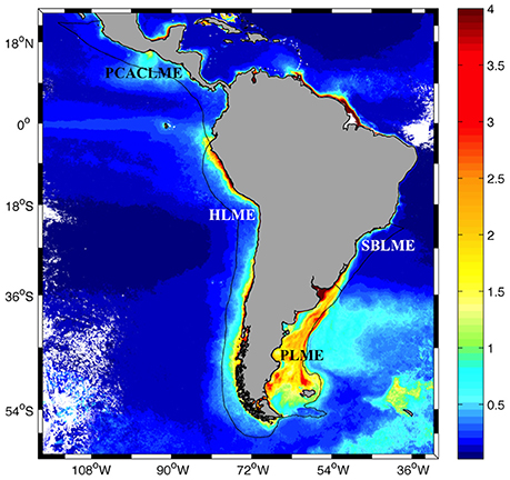
Figure 1. Distribution of SeaWiFS climatological (1997–2006) surface chlorophyll concentrations in austral spring (October–December) around Central and South America (mg m⁻³, 2 km pixel⁻¹). The locations of the South Brazil (SBLME), Patagonia (PLME), Humboldt (HLME), and Pacific Coastal Central American (PCACLME) Large Marine Ecosystems (LMEs) are indicated.

The Humboldt Large Marine Ecosystem (HLME) is an eastern boundary system that extends from northern Peru to southern Chile in the eastern South Pacific Ocean, where it is adjacent to the PLME (Figure 1). The large-scale circulation of the HLME includes the broad eastward flowing West Wind Drift at ~43°S that reaching the coast of South America splits into the equatorward Humboldt Current and the poleward flowing Cape Horn Current (Strub et al., 1998). The oceanic circulation includes a complex pattern of intense surface jets, subsurface undercurrents, and eddies, meanders and filaments, which exchange mass, energy, and biota with the deep ocean (Strub et al., 1998). Ekman offshore divergence due to the trade winds north of ~35°S results in the largest coastal upwelling system in the world, characteristic of this LME. This system shows large oceanographic and climatic variability and is strongly influenced by ENSO (Heileman et al., 2009). About 65% of the area of HMLE corresponds to the Humboldt Current System (HCS) and is under the influence of coastal upwelling from ~4 to 40°S. The fishery off Peru is the most productive in the world, with harvests of anchoveta and sardine that peaked up to 12 million metric tons during 1994. The Chilean fishery concentrates primarily on horse mackerel, anchovy, sardine, and hake (Prado and Drew, 1999). The Cape Horn Current flows poleward along coast of southern Chile (40–55°S) next to a complex fiord system and is mostly under the influence of downwelling-favorable (poleward) winds. The HCS includes an extensive and pronounced oxygen minimum zone (OMZ) centered at 300–400 m and is characterized by high primary production at the surface and a permanent and sharp thermocline that restricts ventilation of subsurface waters (Karstensen et al., 2008) This OMZ has a strong impact on the local ecosystem as well as on global climate through the exchange of greenhouse gases with the atmosphere (Bertrand et al., 2010).

The Pacific Central-American Coastal LME (PCACLME) includes the Pacific Coast of Central America (22°N−4°S) from Mexico to Ecuador and covers ~2 million km². The PCACLME is characterized by recirculating coastal currents and milder temperatures than those of the adjacent California Current and Humboldt Current LMEs. A large part of this LME is under the influence of the meridional displacements of the Inter-tropical Convergence Zone (Bakun et al., 1999) and is also vulnerable to ENSO variability at interannual time scales.

Several studies have observed recent changes in marine environmental conditions at both global and regional scales. Trend analyses of global sea surface temperature (SST) indicate mean increases of 0.71°C century⁻¹ since 1900 (Wu et al., 2012) and between 0.09° ± 0.03 and 0.18° ± 0.04°C decade⁻¹ since the 1980s (Lawrence et al., 2004; Good et al., 2007). Long-term trends in chlorophyll concentrations are variable, with areas of increasing and decreasing chlorophyll around the globe (Gregg et al., 2005; Demarcq, 2009; Saulquin et al., 2013; Boyce et al., 2014; Gregg and Rousseaux, 2014; O'Brien et al., 2017). The factors driving these changes in environmental conditions are not fully understood, and although climate driven changes can have a global effect (i.e., increased SST and more intense stratification), other factors have variable effects on regional scales. It has been shown that climate driven changes of marine ecosystems have a large impact on artisanal fisheries, which in turn have a substantial socio-economic impact in Central and South American countries (e.g., Castilla and Defeo, 2001; Caddy and Defeo, 2003; Defeo et al., 2009; Möller et al., 2009; Schroëder and Castello, 2010). The analysis of longer-term changes in environmental variables is essential for understanding the effects of climate change and ecosystems dynamics on marine populations. The recent increase in the number of ocean color missions allows a great variety of applications, although different durations and timing for the individual missions lead to relatively short datasets that are not appropriate for assessing changes at interdecadal scales. Thus, there is a need for longer time series, which can be obtained by applying a multi-sensor approach.

The VOCES Project (Variability of ocean ecosystems around South America) (CRN 3070) is aimed at assessing the impact of climate variability on the Humboldt, Patagonia, and South Brazil LMEs through collaborative research (http://www.iai.int). The Pacific Central-American Coastal LME is adjacent to HLME and includes the study area of the project “Study of the upwelling system in the Santa Elena Gulf, north Pacific coast of Costa Rica” (CONICIT FV-027-13, Costa Rica). Our study is part of these projects and analyzes the four LMEs as a contribution to the understanding of the processes controlling variability in chlorophyll concentrations and trends around South and Central America. The main objectives of this study are (1) to develop extended time series of satellite chlorophyll concentrations in four LMEs around South and Central America using a combination of SeaWiFS and MODIS high-resolution data, (2) to compare the spatial and temporal patterns and variability observed in chlorophyll concentrations in the different ecosystems, and (3) to determine statistically significant trends in chlorophyll concentrations and discuss their potential implications for the different LMEs.

Materials and Methods

The study area includes the Patagonia (PLME), South Brazil (SBLME), Humboldt (HLME), and Pacific Central American Coastal (PCACLME) Large Marine Ecosystems around South and Central America between 25°N−60°S and 30–120°W (Figure 1). LMEs were defined according to the limits established in http://www.lme.noaa.gov. A preliminary analysis of chlorophyll concentrations within these regions revealed that the limits established originally for PLME excluded part of the shelf-break front where high chlorophyll concentrations of up to ~20 mg m⁻³ often develop during spring and summer (Garcia et al., 2008; Lutz et al., 2010). For this reason, the offshore limit was extended to the 500 m isobath in order to include all high chlorophyll waters in the region.

Daily SeaWiFS Local Area Coverage (LAC) data with 1 × 1 km spatial resolution are available between August 1997 and December 2006. In addition, 9 km pixel⁻¹ data are available until December 2010, when the satellite stopped communicating. The MODIS Aqua dataset includes the period July 2002-present at 1 km pixel⁻¹ and, together, both sensors provide over 20 years of high spatial resolution surface chlorophyll concentration measurements with ~5 years of temporally overlapping data (2002–2006, 54 months). Surface chlorophyll concentrations (CHL, mg m⁻³) from SeaWiFS (SWF) and MODIS Aqua (AQ) were analyzed in the area bounded by 25°N−60°S and 30–120°W. All available high-resolution (~1 km pixel⁻¹) level 2 data were processed with the standard flags and empirical algorithms (OC4v4 for SeaWiFS and OC3M for MODIS, O'Reilly et al., 2000), binned, and mapped to a 2 km pixel⁻¹ spatial resolution. Reprocessing versions 2014.0 (SWF) and 2014.0.1 (AQ) were used. To reduce errors caused by digitization and random noise without losing spatial resolution, a smoothing filter was applied by computing the mean chlorophyll concentration in a 3 × 3 box around each pixel (Hu et al., 2001). Chlorophyll concentrations < 0.02 and >30 mg m⁻³ were excluded from the analyses. Monthly composites were generated from SWF (September 1997–December 2006) and AQ (July 2002-January 2017) data. Data are distributed by the Ocean Biology Processing Group (OBPG) at NASA's Goddard Space Flight Center.

It is well documented that ocean color satellite sensors overestimate chlorophyll concentrations in waters of the Río de la Plata (Figure 1) where high concentrations of sediment and terrigenous material are present (Armstrong et al., 2004; Garcia et al., 2005); thus, this area was excluded from all error and trend analyses. Since there is no significant seasonality in river discharge volume for the Río de la Plata (Piola et al., 2005), years of higher than normal discharge were selected (1998, 2002, 2003, 2010, and 2016; Piola et al., 2008a) and average chlorophyll concentrations for those years were calculated in the area. A mask was defined using the 5 mg m⁻³ isoline as the limit of the river waters and the area included within the mask was excluded from all quantitative analyses.

Previous comparisons of monthly CHL data from SWF and AQ data for the overlapping period (2002–2006) in the Patagonia LME region revealed differences between sensors (Marrari et al., 2016). Preliminary analyses of data for the larger study area included here revealed that in highly productive areas during spring and summer, both estimates agreed well at lower chlorophyll concentrations (< 1 mg m⁻³) but AQ systematically produced larger estimates than SWF at higher values (Figure 2A). For lower productivity waters, SWF produced somewhat higher estimates than AQ, although differences were smaller than for AQ > SWF. The spatial patterns observed in the relationship between SWF and AQ estimates showed a moderate association with the amplitude in spring chlorophyll concentrations (r = 0.525, p < 0.0001; Figure 2B), which in turn is associated with the distribution of spring SST (r = −0.262, p < 0.0001; Figure 2C). In general, warm oligotrophic waters with small spring chlorophyll amplitudes are characterized by higher SWF than AQ estimates, whereas nutrient-rich colder areas that support large phytoplankton blooms and large amplitudes in spring chlorophyll concentrations present the opposite pattern. Based on the high productivity of the LMEs analyzed here and previous reports of SWF performing better than AQ at higher chlorophyll concentrations (e.g., Werdell et al., 2009), the AQ dataset was corrected using SWF as reference. Model II ordinary least squares (OLS) regressions (Legendre and Legendre, 1998) were calculated at all pixels on the log-transformed chlorophyll data using monthly composites for the overlap period, between July 2002 and December 2006. Other analyses with higher order polynomials and other nonlinear fits did not reduce the errors; thus, we present results based on linear fits. Using the coefficients estimated from the regressions, corrections were applied to the entire AQ dataset at all pixels (2002–2017). Taking into consideration the lognormal distribution of chlorophyll data (Campbell, 1995), all error estimates and corrections were made to the log-transformed (base 10) data. The root mean square error (RMS) and bias were calculated at each pixel according to Gregg and Casey (2004) and Marrari et al. (2006):

$\begin{array}{l}log\_RMS=\sqrt{\frac{{\displaystyle \sum {[\log (AQ)-\log (SWF)]}^2}}{n}}\\ \log \_bias=\frac{{\displaystyle \sum [\log \left(AQ\right)-\log \left(SWF\right)]}}{n}\end{array}$

In addition, errors were calculated for different CHL ranges at the different LMEs and compared. Two types of time series were generated at each pixel, each using data from a different sensor for the overlapping period (2002–2006): a first time series combined data from SWF for the entire period available (September 1997–December 2006) with corrected data from AQ for January 2007–January 2017 (TS-A), while the second analysis included SWF data for September 1997–June 2002 and corrected AQ for the entire mission (July 2002–January 2017) (TS-B) (n = 233 months in both cases).

FIGURE 2

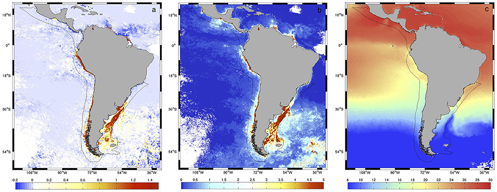
Figure 2. (A) Differences in average spring (October–December) chlorophyll concentration retrievals from SWF and AQUA during the period of overlap of both sensors (2002–2006) (AQ-SWF, mg m⁻³). The geographic limits for the four LMEs analyzed in this study are indicated. (B) Amplitude in climatological spring chlorophyll concentrations from SeaWiFS (maximum-minimum at each pixel, mg m⁻³) for the period 2002–2006 (C) Distribution of average spring sea surface temperature (SST, °C) from MODIS Aqua for the period 2002–2006.

The analysis of trends was done at all pixels jointly for the SWF and AQ time series following the methodology developed in Saulquin et al. (2013). This method considers the noise autocorrelation in the time series, which affects the estimation of the uncertainty in the trend estimate and consequently the ability to detect a significant trend. The time series of chlorophyll concentration, y_t, is modeled as the sum of a long-term linear trend (ω), a seasonal pattern (S_t), and a noise process (N_t) (Weatherhead et al., 1998):

$y_t=\mu +\omega t+S_t+N_t, t=1\dots . n$

where n is the length of the time series and μ is the y-intercept term. N_t is the correlated noise, assumed to be first-order autoregressive process: N_t = ϕN_t−1 + ε_t, with ε_t representing a white noise and ϕ the noise autocorrelation. For two sensors, the assumption is that both datasets share a long-term trend and seasonal pattern but include an unknown level shift, δ, and correlated noise processes. The seasonal component is removed from all time series and the equations are then transformed to remove the autocorrelation (Cochrane and Orcutt, 1949). Spectral analyses conducted on the chlorophyll concentration extended time series show no significant concentration of energy at time periods longer than 12 months. Therefore, we have not included an interannual component other than the linear trend.

For periods when only one time series is available, the equations for SeaWiFS ($y_{1t}^{\ast }$) and MODIS ($y_{2t}^{\ast }$) are:

$\begin{array}{l}{y}_{1t}^{*}= \mu \left(1-{\varphi }_1\right)+\omega {\varphi }_1+\omega \left(1-{\varphi }_1\right)t+{\epsilon }_{1t}\\ y_{2t}^{*}= \mu \left(1-{\varphi }_2\right)+\omega {\varphi }_2+\omega \left(1-{\varphi }_2\right)t+\delta \left(1-{\varphi }_2\right)+{\epsilon }_{2t}\end{array}$

where t is time relative to each time series. When both time series are available:

$y_t^{*}= \mu \left(1-\alpha \right)+\omega \left(1-\alpha \right)t-\alpha \delta +{\epsilon }_{3t}$

with α representing the correlation between N₁ and N₂. The transformed equation can be expressed in matrix form as:

$Y^{*}= X^{*}A+\epsilon$

where X* is the Tx3 coefficient matrix for the equation system, A is the parameter vector (μ, δ, ω), and ε is the residual white noise. The OLS estimator of A yields estimates of μ, δ, and ω. In practice, the equation is solved through iteration until convergence, with initial parameter values estimated from the data. Then, all parameters are revaluated. The variable |ω|/σ_ω is used to detect significant trends, and the 95% confidence level is reached for |ω|/σ_ω > 1.96. Only trends satisfying the 95% detection threshold are considered in the analyses. More details on the numerical resolution of the equations can be found in Tiao et al. (1990) and Saulquin et al. (2013).

Results

The correction of the AQ dataset (AQ_corr) improved the relationship between SWF and AQ for most of the region and allowed the combination of SWF and AQ_corr data to develop the longest time series of high-resolution chlorophyll concentrations in the region to date. Although the correction did not greatly improve the root mean squared error (log_RMS) for the SWF vs. AQ regression, the bias (log_Bias) was significantly reduced in the entire study area and the ratios AQ/SWF were greatly improved (closer to 1) for all LMEs examined (Figure 3 and Table 1).

FIGURE 3

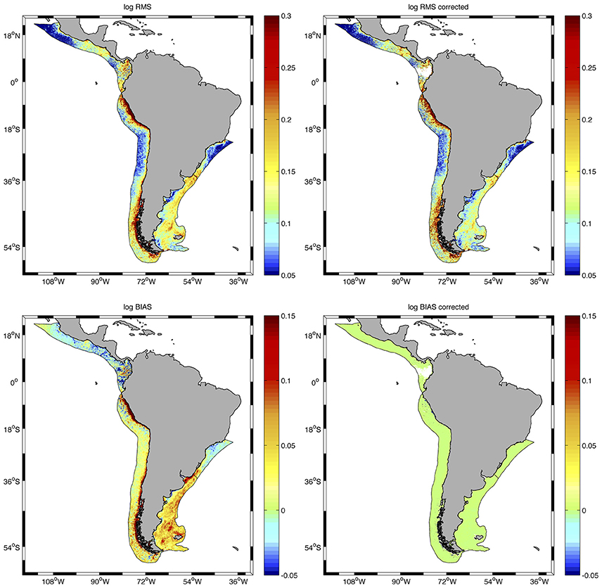
Figure 3. Distribution of root mean squared error (log_RMS) (upper panels) and bias (lower panels) for the regression of SWF vs. AQ chlorophyll concentrations before (left) and after (right) correction of the AQ dataset at all pixels in the LMEs examined. Statistics are presented in Table 1.

TABLE 1

Table 1. Area (km²), mean ± standard deviation (SD) spring (October–December) chlorophyll concentration (mg m⁻³) and SST (°C) from MODIS Aqua (2007–2017) for the LMEs analyzed.

The differences between SeaWiFS and MODIS retrievals varied between LMEs, with the highest ratios AQ/SWF occurring in HLME followed by SBLME and PLME, and the best agreement observed at PCACLME. Before applying the corrections to AQ, the ratio AQ/SWF was >1 for the entire chlorophyll concentration range at HLME and PLME. High ratios between 1.30 and 1.57 (indicating an overestimation of AQ relative to SWF of 30–57%) occurred for chlorophyll concentration values between 1 and 9 mg m⁻³ at HLME. At SBLME, an overestimation ranging between 10 and 20% was observed for chlorophyll concentrations between 1.5 and 8 mg m⁻³, while at PLME, ratios of ~1.15 occurred between 1 and 6 mg m⁻³ (Figure 4A). On the other hand, for PCACLME, AQ/SWF ratios were ~1 for most of the chlorophyll concentration range examined, only decreasing to values < 1 at >5 mg m⁻³. After applying the corrections, the relationship between sensor retrievals was greatly improved, with ratios AQ_corr/SWF closer to 1 for all chlorophyll concentration values examined at all LMEs (Figure 4B). For HLME, AQ_corr/SWF remained high (~1.2) for chlorophyll values within the 1.5–4 mg m⁻³ range.

FIGURE 4

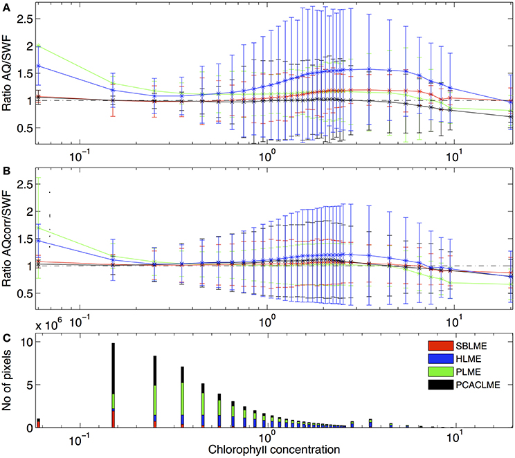
Figure 4. Mean ratio of (A) AQ/SWF before and (B) after correction of the AQ dataset as a function of chlorophyll concentration ranges (mg m⁻³) from SWF for the period 2002–2006 at the LMEs examined: PLME (green), SBLME (red), HLME (blue) and PCACLME (black). Error bars represent 1 standard deviation. (C) Frequency of SWF chlorophyll concentration values at each LME.

The distribution of ratios AQ/SWF before and after correction of AQ showed some interesting spatial patterns (Figure 5). Before corrections, AQ/SWF ratios were predominantly >1 at PLME and HLME, and mostly < 1 at SBLME and PCACLME, in coincidence with the spatial patterns observed in chlorophyll concentrations at those LMEs, which are evident from the spring climatology presented in Figure 1. In areas where chlorophyll reaches high spring and summer values, AQ tends to overestimate concentrations relative to SWF, whereas the opposite is true for areas where chlorophyll concentrations remain relatively low, such as the mostly subtropical SBLME and the tropical PCACLME areas. It is interesting to note that even though the mean ratio AQ/SWF at SBLME was >1 for most of the chlorophyll range examined (Figure 4A), the majority of the pixels (63.89%) had values < 1 (Figure 5A). After applying corrections, ratios became closer to 1 at all LMEs, except for some areas of HLME where the ratios AQ_corr/SWF >1 observed in Figure 4B are evident (Figure 5B).

FIGURE 5

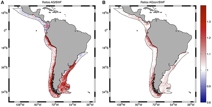
Figure 5. Spatial distribution of the ratio AQ/SWF before (A) and after (B) correcting the AQ dataset at all pixels in the LMEs examined. Statistics are presented in Table 1.

The correction of AQ and improvement of the agreement between sensors allowed the combination of both datasets to generate extended time series of chlorophyll concentrations at all pixels of the LMEs examined. The newly extended time series TS-A and TS-B represent the longest records of high-resolution chlorophyll concentration data in the region. At each LME, monthly mean chlorophyll concentrations were calculated and time series were generated, which revealed important differences between the regions examined for both sets of time series (Figure 6). For both TS-A (SWF 1997–2006 + AQ_corr 2007–2017), and TS-B (SWF 2997–2002 + AQ_corr 2002–2017), the highest monthly mean chlorophyll concentrations occurred consistently at PLME, followed by HLME and SBLME, while the lowest values were prevalent at PCACLME. Even though overall chlorophyll concentrations at HLME were higher than those at SBLME, chlorophyll maxima were regularly higher at the latter, most likely driven by the high winter values often observed in the southern part of SBLME. A seasonal pattern was evident in all regions, although more marked at PLME and SBLME, with peaks during austral spring for PLME (October–December) and HLME (September–November) (Figure 6). Maxima at SBLME occurred during July–September, in coincidence with the period of maximum extension of the Río de la Plata river plume, whereas at PCACLME, they were observed during late boreal winter-early spring (February–April). For both TS-A and TS-B, significant increasing trends were observed in the areal mean chlorophyll concentrations at PLME and HLME, whereas no trends were detected at SBLME or PCACLME (Table 2). The strongest positive trends occurred at PLME (0.0032 mg m⁻³ month⁻¹ for both TS-A and TS-B) and HLME (0.0009 mg m⁻³ month⁻¹ for TS-A and TS-B) and represent average increases of ~66% and 32% since 1997, respectively.

FIGURE 6

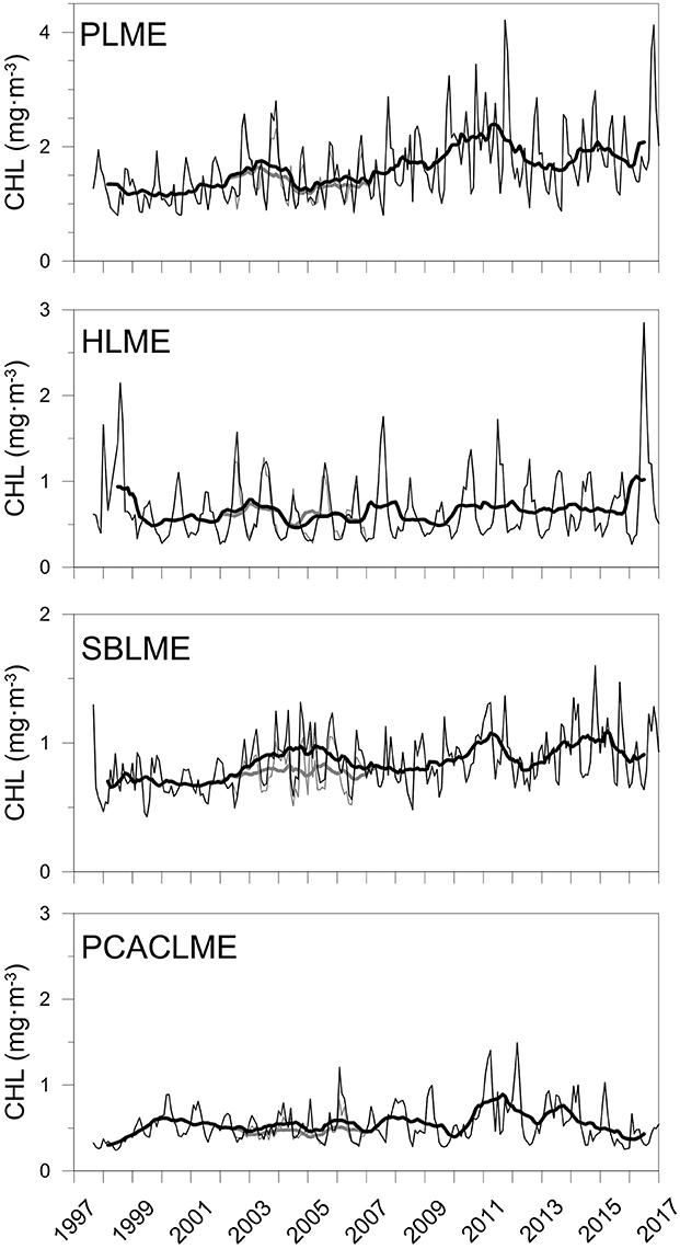
Figure 6. Extended time series (1997–2017) of monthly mean CHL (mg m⁻³, n = 233) at the PLME, HLME, SBLME, and PCACLME using a combination of SWF data for the period September 1997-December 2006 and AQ_corr for January 2007-January 2017 (TS-A, gray), and SWF data for September 1997-June 2002 and AQ_corr for July 2002-January 2017 (TS-B, black). The thick lines represent the 13-month running mean. Regression parameters are presented in Table 2.

TABLE 2

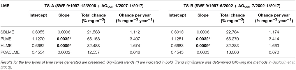
Table 2. Regression parameters for extended time series of monthly mean chlorophyll concentrations at the four LMEs analyzed for the period September 1997-January 2017 (n = 233 months).

To further examine the differences between the LMEs, an analysis of the climatology of monthly mean chlorophyll concentrations (1997–2017) clearly shows the highest values at PLME throughout the year, with austral spring and summer concentrations up to 2.5 times higher than any other LMEs, followed by HLME during austral spring, summer and fall (Figure 7). During winter, SBLME shows higher average concentrations than HLME, with climatological areal mean values of 1.19 and 1.17 mg m⁻³ for July and August, respectively. PCACLME presented the lowest monthly chlorophyll concentrations of all LMEs during austral winter and spring, but slightly higher values than SBLME during summer and fall. It is interesting to note that PLME and SBLME had the highest seasonality, with peaks in austral spring and winter, respectively, while both HLME and PCACLME showed little to no seasonal variability in chlorophyll concentrations (Figure 7).

FIGURE 7

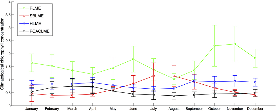
Figure 7. Monthly climatological chlorophyll concentrations (mg m⁻³) for the period September 1997-January 2017 using TS-A (SeaWiFS data for 1997–2006 and MODIS Aqua data for 2007–2017). For each LME, values represent the climatology of the areal mean chlorophyll concentration for each month. Errorbars represent 1 standard deviation.

A more detailed analysis of the spatial distribution of trends within each LME revealed that significant trends occurred in 78.23% of PLME and 43.03% of HLME, whereas only smaller subareas of SBLME (26.35%) and PCACLME (13.35%) showed significant changes since 1997 (Table 3). The largest trends were observed at PLME (median slope = 0.0011 mg m⁻³ month⁻¹), where 99.22% of the pixels with significant trends showed increasing chlorophyll concentrations (Figure 8). At HLME, the median trend was 0.0009 mg m⁻³ month⁻¹, and again 88.98% presented positive values. For SBLME and PCACLME, changes in chlorophyll concentrations over time were less evident. At SBLME, 26.35% of the pixels showed significant trends, 97.69% of which were positive. The median trend for SBLME was 0.0005 mg m⁻³ month⁻¹, while at PCACLME the median trend was 0.0011 mg m⁻³ month⁻¹ but only 13.35% of the pixels showed changes corresponding to 62.64% increases and 37.36% decreases in overall chlorophyll concentrations since 1997 (Figure 8 and Table 3).

TABLE 3

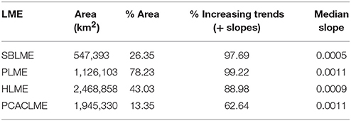
Table 3. Statistics for the trends estimated at the four LMEs examined, including the area of each LME (km²), the percentage (%) of the area that presented significant trends, the percentage (%) of those significant trends that were positive (increasing chlorophyll concentrations), and the median trend for each LME (mg m⁻³ month⁻¹).

FIGURE 8

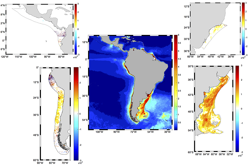
Figure 8. Spatial distribution of significant trends in CHL (mg m⁻³ month⁻¹) in the four LMEs examined around South and Central America for the period 1997–2017. The central panel presents the distribution of climatological spring chlorophyll concentrations from MODIS Aqua for the period 2002–2017 (mg m⁻³). Black solid lines represent the limits of each LME. White areas in LME panels indicate that the trend is not significantly different from zero at the 95% confidence level. Statistics for each LME are presented in Table 3.

Discussion

Variability in Chlorophyll Concentrations

Globally, the distribution of phytoplankton is primarily controlled by the degree of stratification, which in turn affects nutrient supply and light exposure: while in warm and permanently stratified waters nutrients limit phytoplankton growth, in seasonally stratified areas, nutrient-rich waters from below the mixed layer supply nutrients to the illuminated layer after the breakdown of the thermocline, supporting phytoplankton growth during spring and summer (Behrenfeld et al., 2006; Doney, 2006). The comparison of average conditions between LMEs confirmed this inverse relationship between surface temperature and chlorophyll, with the coldest area (PLME) supporting the highest chlorophyll concentrations and seasonality in the study area. At PLME the maximum climatological monthly CHL concentration of 2.76 mg m⁻³ was observed in November, and a minimum of 1.15 mg m⁻³ in August, which is noteworthy considering this value is higher than the maxima observed at HLME and PCACLME, and very similar to the maximum at SBLME. The high productivity of PLME has been long recognized, especially in the shelf-break area where large blooms develop during summer, supporting some of the largest fisheries in the world and serving as foraging areas for higher trophic levels (e.g., Campagna et al., 2006).

HLME has been characterized as moderately productive, even though localized areas of high productivity occur along the coast (Heileman et al., 2009). HLME includes a large area of wide latitudinal range and high spatial variability in physical and biological processes: while the northern part is affected by ENSO, the southern sector is not directly impacted by this phenomenon. The most prominent area is the HCS, one of the four major global eastern boundary current systems, characterized by coastal upwelling of cool nutrient-rich waters and dramatically increased biological production, including ~10% of the global fish catch (Chavez et al., 2008). High variability in this region is associated with ENSO, with El Niño (warm) conditions resulting in elevated sea level, a deeper thermocline, and warmer temperatures. Alongshore winds and offshore Ekman transport persist during El Niño (Carr et al., 2002; Escribano et al., 2004), but bring waters from above the deepened thermocline, which is nutrient-depleted, resulting in decreased production. On average, HLME supports about half of the monthly mean chlorophyll concentration of PLME throughout the year, with monthly climatological chlorophyll concentrations ranging between 0.75 and 1.8 mg m⁻³, and an overall ratio PLME/HLME of 1.92 ± 0.44. However, HLME encompasses about twice the area, which translates into a monthly mean integrated chlorophyll concentration 14% higher than that recorded at PLME. In addition, HLME presents low seasonality, with the variability between monthly chlorophyll values being ~25% of that observed at PLME, and comparable to that of the oligotrophic PCACLME. Previous studies showed that off northern Chile, chlorophyll concentrations are somewhat higher in winter and early spring, while in central southern Chile (30–40°S), the chlorophyll peak develops during the summer months (Thomas et al., 2001). Another study observed a peak in biomass during summer north of 22°S and during spring further south, with maximum values >5 mg m⁻³ north of 20°S and south of 35°S. Primary production followed the same pattern, with minimum values (~2 g C m⁻² day⁻¹) in the central area of HLME (~27°S) and maxima north of 18°S and south of 34°S (>4 g C m⁻² day⁻¹) (Carr and Kearns, 2003).

At PCACLME, SST values are the highest and chlorophyll concentrations the lowest of the LMEs analyzed. Waters in this region are permanently stratified and nutrient availability limits photosynthesis throughout the year. Chlorophyll concentrations at PCACLME remain relatively low throughout the year and do not exceed 0.66 mg m⁻³ for the climatological monthly mean. However, within PCACLME there are areas of localized increased chlorophyll concentrations as a result of a combination of regional atmospheric and oceanographic processes. The Gulf of Papagayo on the Pacific coast of Costa Rica, for example, is a dynamic area characterized by high seasonal productivity and sustains ~45% of the fisheries in the country (www.incopesca.go.cr). Other localized areas of high production include the Gulf of Tehuantepec off Mexico and the Gulf of Panama. In these regions, primary production is determined by vertical mixing and upwelling, which supply nitrate-rich waters to the surface. The regional climate is dominated by the north-south migration of the Intertropical Convergence Zone (ITCZ) located between the equator and 10°N and by the influence of cold air masses moving in from North America. During boreal winter (December–February), the ITCZ moves south, the easterlies intensify, and cold fronts move through the Caribbean, leading to strong winds blowing from the Atlantic to the Pacific Ocean and inducing coastal upwelling and the formation of large cyclonic and anticyclonic eddies that propagate offshore. The result is a sharp increase in coastal chlorophyll concentrations that can extend up to 900 km offshore and have a strong influence on the biology of the area (McClain et al., 2002). Results from numerical models reproduce the variability observed in chlorophyll concentrations and its relationship with Ekman pumping velocities and ENSO (Sasai et al., 2012).

SBLME is the smallest of the LMEs examined here and presented intermediate chlorophyll concentrations. In austral fall and winter freshwater runoff from the Río de La Plata and Lagoa dos Patos move northward along the coast supplying nutrients to the area and promoting primary production in the southern sector of the SBLME (Brandini, 1990). In addition, SBLME showed moderate seasonal variability, with a winter peak in chlorophyll concentrations that can be accounted for by the tongue of chlorophyll-rich waters from the Río de la Plata that migrate northward along the coast and lead to high chlorophyll concentrations of up to >3.5 mg m⁻³ in this area (Garcia and Garcia, 2008; Piola et al., 2008b). Although high concentrations of suspended matter likely cause an overestimation of chlorophyll in the estuary, in situ data have confirmed that the Río de la Plata supports values of up to 7.7 mg m⁻³ (e.g., Carreto et al., 1986). Our results agree with previous studies that indicate that the slope and continental shelf in the northern part of SBLME are characterized by low chlorophyll concentrations throughout the year (Brandini, 1990; Castro et al., 2006).

Trends in Large Marine Ecosystems

The corrections made to the MODIS Aqua dataset in this study allowed the combination of multi-sensor data to generate the longest time series of satellite chlorophyll concentrations available to date around South and Western Central America. The newly developed extended time series include almost 20 years of data at high spatial resolution and revealed significant trends in chlorophyll concentrations. Previous studies observed varying trends in global average chlorophyll concentrations, with reports of a general decline (e.g., Behrenfeld et al., 2006; Vantrepotte and Mélin, 2009; Boyce et al., 2014; Lorenzoni et al., 2017), as well as no detectable trends (Beaulieu et al., 2013) or even a global increase of 4.13% (Gregg et al., 2005). However, there is general consensus in that there is high global variability, with regions of increasing and decreasing trends. For example, Hammond et al. (2017) detected a small global decline in chlorophyll between 1997 and 2013, but observed regional variability with both positive and negative trends present across the globe ranging from ~−2 to 1% year⁻¹. Our results indicate that within the LMEs analyzed the greatest changes have occurred at the Patagonia (PLME) and Humboldt (HLME) Large Marine Ecosystems, where the largest and almost exclusively increasing trends were recorded and the largest percent areas showed significant changes. On the other hand, the warmer SBLME and PCACLME showed no significant trends in areal mean chlorophyll concentrations, and only smaller percent areas showed significant trends. The increasing chlorophyll concentrations observed on the Patagonian Shelf and in the Humboldt upwelling system have been reported in previous global studies (Gregg et al., 2005; Saulquin et al., 2013; Siegel et al., 2013; Muller-Karger et al., 2017), although these analyses were based on shorter time series with coarser resolution. The high resolution data used in this study allows a more detailed analysis of the variability in the distribution of trends within the LMEs and the relationship with other variables, leading to a better understanding of the mechanisms controlling chlorophyll distribution and the changes occurring over the past two decades.

At PMLE, maximum chlorophyll concentrations occur during austral summer over the mid-shelf and in proximity of the shelf-break, where a sharp thermal front system develops separating vertically stratified warm shelf waters from weakly stratified waters of the Malvinas Current (Acha et al., 2004; Romero et al., 2006). Our results revealed that large positive trends also occurred mostly in these areas that support high spring and summer chlorophyll, suggesting that the processes that favor production most likely have intensified. Although rich in nutrients, the Malvinas Current is characterized by low phytoplankton abundances presumably due to intense mixing and light limitation. On the seasonally stratified shelf, phytoplankton growth is limited by nutrient concentrations. As the Malvinas Current flows northward, upwelling along the shelf-break supplies cold nutrient-rich waters onto the shelf (Matano and Palma, 2008; Piola et al., 2010; Valla and Piola, 2015) favoring increased primary production in the vicinity of the shelf break and adjacent shelf waters. Model results suggest that the Malvinas Current controls cross-shelf exchanges at the shelf-break as well as the circulation over the continental shelf (Matano et al., 2010). In turn, the shelf break upwelling is controlled by the along-shelf pressure gradient associated with the presence of a slope current (Matano and Palma, 2008). The increasing trends observed in the shelf-break area and over the continental shelf could be an indication of changes affecting the supply of nutrients onto the shelf via changes in the interaction between the shelf break and the Malvinas Current (e.g., Matano and Palma, 2008). Alternatively, changes in along-slope winds over the outer shelf can modulate the intensity and location of shelf break upwelling (e.g., Carranza et al., 2017). To the best of our knowledge there are no published reports of increased transport of the Malvinas Current or changes in the along-slope winds that might lead to a more intense upwelling during the last two decades. The factors leading to the large positive trends in chlorophyll in the PLME should be further investigated.

Most of HMLE also presented increasing trends in chlorophyll concentrations. Based on the primary productivity of coastal waters, previous studies described four provinces along HLME (Montecino and Pizarro, 2006; Quiñones et al., 2009; Gutiérrez et al., 2016). The most productive province is located off Peru, followed by the area off central Chile, which shows stronger seasonality associated with changes in wind stress. The coastal areas off northern Chile and the Magellanic region have the lowest production rates. This description coincides, in general, with the spatial distribution of CHL trends observed at HLME, where the largest positive trends occurred off Peru and central Chile, smaller increases were observed off northern Chile, and no trends were detected off the southern Chilean coast, in the area under the influence of the Cape Horn Current. North of 40°S, the increasing trends in chlorophyll concentrations were associated with negative trends in SST. HLME is one of two LMEs in the world showing a cooling trend, the other being the California Current LME (Chavez et al., 2008; Belkin, 2009). Within HLME, there are two regions of persistent cooling close to the continent: a larger one off northern Chile and southern Peru (~10–30°S) and a smaller one at ~40–50°S (Gutiérrez et al., 2016; Thompson et al., 2017), which largely coincide with the areas of maximum positive trends in chlorophyll. HLME is under the influence of the Humboldt upwelling system, where cold nutrient-rich waters from below the thermocline are upwelled to the surface as a result of the prevailing easterlies, favoring increased phytoplankton concentrations. It has been suggested that upwelling intensity has increased as a result of climate change (Bakun, 1990; Demarcq, 2009; Sydeman et al., 2014), and that an observed cooling of 0.10°C for the period 1982–2006 is the result of increased upwelling, which ultimately translates into higher nutrient supply and chlorophyll concentrations in the area (Belkin, 2009). Gutiérrez et al. (2011) used sediment core data spanning 150 years to reconstruct the SST record from an upwelling area off Peru and confirmed a temperature decrease since the 1950s, which was in phase with an increase in productivity and also coincided with strengthened alongshore winds and intensified upwelling.

Global warming has the potential to increase stratification, affecting phytoplankton distribution and abundance and has been suggested as the cause of the expansion of the low-chlorophyll, low-productivity central ocean gyres (McClain et al., 2004; Polovina et al., 2008; Irwin and Oliver, 2009). Signorini et al. (2015) used a combination of satellite and model data to analyze trends in chlorophyll concentration, primary production, SST, mixed layer depth (MLD), and sea level anomaly (SLA) in five oligotrophic gyres for the period 1998–2013. They observed that, in general, the oligotrophic waters are expanding, with positive trends in SST, MLD and SLA, and reduced chlorophyll concentrations and primary production, with important implications for atmospheric CO₂ uptake and the biological pump. In an analysis of SST change in the world ocean LMEs, SBLME showed the strongest warming among the four LME's considered here, with a net increase in SST of 0.53°C during the period 1982–2006, while PCACLME and PLME showed milder changes of 0.14 and 0.08°C, respectively (Belkin, 2009). The observation of mostly positive trends in chlorophyll concentrations at the four LMEs examined in this study is an unexpected result considering the general surface warming recorded for the global ocean. A recent IOC-UNESCO report that examined global trends in SST and chlorophyll concentrations for the period 1998–2012 using monthly averaged satellite data with a 0.5° × 0.5° spatial resolution described mixed relationships, with warming and cooling areas associated with both increasing and decreasing chlorophyll concentrations (O'Brien et al., 2017). In general, reduced chlorophyll concentrations associated with warmer SSTs can be explained in terms of increased vertical stability and changes in mixed layer depth (e.g., Behrenfeld et al., 2006). As the surface layer warms, the mixed layer becomes shallower and the thermocline stronger, which constrains the nutrient input from sub-thermocline water and ultimately reduces phytoplankton abundance. However, although most of our study area showed warming trends, decreasing chlorophyll concentrations were only observed in a small area of PCACLME. This suggests that no single factor can be identified as controlling changes in these LMEs but that a variety of mechanisms besides changes in stratification and mixed layer depth due to warming must be operating regionally at different scales. An alternative proposed mechanism that might explain, at least in part, increasing chlorophyll concentrations in a warming environment include changes in the composition and physiology of the phytoplankton community. Behrenfeld et al. (2015) pointed out that due to photoacclimation, chlorophyll variability is not simply a measure of phytoplankton biomass, but is also modulated by changes in pigmentation and as a physiological response to variability in nutrient supply. The study also concluded that relationships between trends in chlorophyll concentration and ocean warming do not represent proportional changes in primary production, as declines in chlorophyll can be related to constant or increased photosynthesis.

Implications for Higher Trophic Levels

The changes occurring in SST and chlorophyll concentrations have important implications for ecosystem dynamics and trophic interactions. For fish and many invertebrates, the highest mortality occurs during the early developmental stages of egg and larva, which are highly susceptible to changes in environmental conditions, such as temperature and oxygen concentrations, food availability (i.e., phyto- and zooplankton concentrations), and physical processes (turbulence and advection) (Cushing, 1975; Cury and Roy, 1989; Bakun, 1998; Mann and Lazier, 2005). Fluctuations in the environment will affect the timing of the onset of the spring bloom, with early or delayed blooms having a negative impact on the survival of fish larvae and recruitment (match-mismatch hypothesis, Cushing, 1990). Previous studies have shown that interannual variability in chlorophyll concentrations during the reproductive season can have strong effects on recruitment (Platt et al., 2003; Fuentes-Yaco et al., 2007; Marrari et al., 2008, 2013), with not only the concentration of chlorophyll having an effect on reproductive success, but also other aspects of phytoplankton dynamics, such as the timing and duration of the spring bloom. At HLME, the fish community is dominated by four pelagic species: the anchoveta Engraulis ringens, the sardine Sardinops sagax, the jack mackerel Trachurus murphyi, and the chub mackerel Scomber japonicus. These species feed on phytoplankton and/or zooplankton for part or all of their life cycles; thus, changes in the abundance and composition of the phytoplankton community can have a direct impact on their population via changes in the availability of food.

At PLME, the increases in chlorophyll concentrations observed at the shelf break and in some coastal areas are of special interest in terms of fisheries. The northern population of the argentine anchovy Engraulis anchoita spawns in coastal waters shallower than ~50 m between 34 and 41°S, in the vicinity of a thermal front that separates mixed coastal waters from seasonally stratified mid-shelf waters. At the front, high chlorophyll concentrations develop during spring. A recent study showed that variability in the timing, magnitude, and duration of the spring bloom explained a large fraction of the variability in anchovy recruitment (Marrari et al., 2013). On the other hand, the area of Isla Escondida and the San Jorge Gulf (43–47°S) represent the main spawning and nursery grounds for the argentine hake Merluccius hubbsi, the main demersal fishery in the region. Recent results indicated that larval survival was related to spring chlorophyll concentrations and the timing of the chlorophyll maximum in the main spawning area, suggesting that phytoplankton dynamics likely affects the reproductive success of hake via de production of zooplanktonic prey for the larvae (Marrari et al., under review).

Changes in phytoplankton abundances can have a direct effect on the biological pump and global carbon budget. Kahl et al. (2017) analyzed the distribution of sea-air CO₂ fluxes on the Patagonia shelf and observed that on the mid- and outer-shelf areas fluxes were dominated by biological processes, leading to a strong sink of atmospheric CO₂ of −6.0 × 10⁻³ m⁻² day⁻¹, equivalent to −20 TgC year⁻¹, with the maximum uptake occurring in spring. This suggests that an analysis of the seasonality in the trends observed should be included in future studies to more accurately describe the effects of long-term changes in chlorophyll concentrations on the ecosystem. Increased phytoplankton abundances will intensify carbon export to the deep ocean with a direct effect on benthic-pelagic interactions. Franco et al. (2017) used particle-tracking models and observed that 80% of the particles released at the surface in proximity of shelf break at PLME settled on the bottom in areas where scallop beds are known to occur; thus an increase in surface phytoplankton abundances could positively impact benthic communities.

The changes occurring in chlorophyll concentrations over the last two decades have important ecological and economic implications for marine populations. In light of the ongoing climate change, further changes in phytoplankton dynamics are anticipated. This highlights the need to continue the analysis of trend in key environmental variables in order to better understand and predict the effects on ecosystem dynamics and the economy of the LMEs.

Author Contributions

All authors (MM, AP, and DV) contributed substantially to the design of this study, the analysis of the data, drafting the work, interpreting results and revising it critically. All authors have approved the final version and agreed to be accountable for all aspects of the work in ensuring that questions related to the accuracy or integrity of any part of the work are appropriately investigated and resolved.

Conflict of Interest Statement

The authors declare that the research was conducted in the absence of any commercial or financial relationships that could be construed as a potential conflict of interest.

Acknowledgments

We thank John Wilding for assisting with data processing. SeaWiFS and MODIS data were distributed by the NASA Ocean Biology Processing Group. This study was funded by grants PICT-2013-1243 from Fondo para la Investigación Científica y Tecnológica (Argentina) and CRN3070 from the Inter-American Institute for Global Change Research through the US National Science Foundation grant GEO-1128040.

References

Acha, E. M., Mianzán, H. W., Guerrero, R. A., Favero, M., and Bava, J. (2004). Marine fronts at the continental shelves of austral South America. Physical and ecological processes. J. Mar. Syst. 44, 83–105. doi: 10.1016/j.jmarsys.2003.09.005

CrossRef Full Text | Google Scholar

Acha, E. M., Simionato, C. G., Carozza, C., and Mianzán, H. W. (2012). Climate-induced year-class fluctuations of whitemouth croaker Micropogonias furnieri (Pisces, Sciaenidae) in the Rio de la Plata estuary, Argentina-Uruguay. Fish. Oceanogr. 21, 58–77. doi: 10.1111/j.1365-2419.2011.00609.x

CrossRef Full Text | Google Scholar

Armstrong, R. A., Gilbes, F., Guerrero, R., Lasta, C., Benavidez, H., and Mianzán, H. (2004). Validation of SeaWiFS-derived chlorophyll for the Rio de la Plata Estuary and adjacent waters. Int. J. Remote Sens. 25, 1501–1505. doi: 10.1080/01431160310001592517

CrossRef Full Text | Google Scholar

Bakun, A. (1990). Global climate change and intensification of coastal ocean upwelling. Science 247, 198–201. doi: 10.1126/science.247.4939.198

PubMed Abstract | CrossRef Full Text | Google Scholar

Bakun, A. (1998). “Ocean triads and radical interdecadal stock variability: bane and boon for fishery management science,” in Reinventing Fisheries Management, eds T. J. Pitcher, P. J. B. Hart, and D. Pauly (Dordrecht: Kluwer Academic Publishers), 331–358.

Bakun, A., Csirke, J., Lluch-Belda, D., and Steer-Ruiz, R. (1999). “The Pacific Central American coastal LME,” in Large Marine Ecosystems of the Pacific Rim: Assessment, Sustainability and Management, eds K. Sherman and Q. Tang (Malden: Blackwell Science Inc.,), 268–280.

Beaulieu, C., Henson, S. A., Sarmiento, J. L., Dunne, J. P., Doney, S. C., Rykaczewski, R. R., et al. (2013). Factors challenging our ability to detect long-term trends in ocean chlorophyll. Biogeosciences 10, 2711–2724. doi: 10.5194/bg-10-2711-2013

CrossRef Full Text | Google Scholar

Behrenfeld, M. J., O'Malley, R. T., Boss, E. S., Westberry, T. K., Graff, J. R., Halsey, K. H., et al. (2015). Revaluating ocean warming impacts on global phytoplankton. Nat. Clim. Chang. 6, 323–330. doi: 10.1038/nclimate2838

CrossRef Full Text | Google Scholar

Behrenfeld, M. J., O'Malley, R. T., Siegel, D. A., McClain, C. R., Sarmiento, J. L., Feldman, G., et al. (2006). Climate-driven trends in contemporary ocean productivity. Nature 444, 752–755. doi: 10.1038/nature05317

PubMed Abstract | CrossRef Full Text | Google Scholar

Belkin, I. M. (2009). Rapid warming of large marine ecosystems. Prog. Oceanogr. 81, 207–213. doi: 10.1016/j.pocean.2009.04.011

CrossRef Full Text | Google Scholar

Bertrand, A., Fréon, P., Chaigneau, A., Echevin, V., Estrella, C., Demarcq, H., et al. (2010). Impactos del Cambio Climático en las Dinámicas Oceánicas, el Funcionamiento de los Ecosistemas y las Pesquerías en el Perú: Proyección de Escenarios e Impactos Socio Económicos. Embajada Británica en Lima. Available online at: http://humboldt.iwlearn.org/en/information-and-publication-1/Bertrandetal2010escenariospesquerosCCPeru.pdf.

Bianchi, A. A., Bianucci, L., Piola, A. R., Ruiz Pino, D., Schloss, I., Poisson, A., et al. (2005). Vertical stratification and air–sea CO₂ fluxes in the Patagonian shelf. J. Geophys. Res. 110:C07003. doi: 10.1029/2004JC002488

CrossRef Full Text | Google Scholar

Bianchi, A. A., Ruiz Pino, D., Isbert Perlender, H. G., Osiroff, A. P., Segura, V., Lutz, V., et al. (2009). Annual balance and seasonal variability of sea–air CO₂ fluxes in the Patagonian Sea: their relationship with fronts and chlorophyll distribution. J. Geophys. Res. 114:C03018. doi: 10.1029/2008JC004854

CrossRef Full Text | Google Scholar

Boyce, D. G., Dowd, M., Lewis, M. R., and Worm, B. (2014). Estimating global chlorophyll changes over the past century. Prog. Oceanogr. 122, 163–173. doi: 10.1016/j.pocean.2014.01.004

CrossRef Full Text | Google Scholar

Brander, K. M. (2007). Global fish production and climate change. Proc. Natl. Acad. Sci. U.S.A. 104, 19709–19714. doi: 10.1073/pnas.0702059104

PubMed Abstract | CrossRef Full Text | Google Scholar

Brandini, F., Boltovskoy, D., Piola, A. R., Kocmur, S., Rottgers, R., Abreu, P., et al. (2000). Multiannual trends in fronts and distribution of nutrients and chlorophyll in the southwestern Atlantic. Deep Sea Res. I 47, 1015–1033. doi: 10.1016/S0967-0637(99)00075-8

CrossRef Full Text | Google Scholar

Brandini, F. P. (1990). Hydrography and characteristics of the phytoplankton in shelf and oceanic waters off southeastern Brazil during winter (July/August 1982) and summer (February/March 1984). Hydrobiologia 196, 111–148. doi: 10.1007/BF00006105

CrossRef Full Text | Google Scholar

Caddy, J. F., and Defeo, O. (2003). Enhancing or Restoring the Productivity of Natural Populations of Shellfish and Other Marine Invertebrate Resources. FAO Fisheries Technical Paper, Vol. 448. (Rome: FAO), 159.

Google Scholar

Campagna, C., Piola, A. R., Marin, M. R., Lewis, M., and Fernández, T. (2006). Southern elephant seal trajectories, ocean fronts and eddies in the Brazil/Malvinas Confluence. Deep Sea Res. I 53, 1907–1924. doi: 10.1016/j.dsr.2006.08.015

CrossRef Full Text | Google Scholar

Campbell, J. W. (1995). The lognormal distribution as a model for bio-optical variability in the sea. J. Geophys. Res. 100, 13237–13254. doi: 10.1029/95JC00458

CrossRef Full Text | Google Scholar

Campos, P., Möller, O. O., Piola, A. R., and Palma, E. D. (2013). Seasonal variability and western boundary upwelling: cape Santa Marta (Brazil). J. Geophys. Res. Oceans 118, 1420–1433. doi: 10.1002/jgrc.20131

CrossRef Full Text

Carr, M. E., and Kearns, E. J. (2003). Production regimes in four eastern boundary current systems. Deep Sea Res. II 50, 3199–3221. doi: 10.1016/j.dsr2.2003.07.015

CrossRef Full Text | Google Scholar

Carr, M. E., Strub, P. T., Thomas, A. C., and Blanco, J. L. (2002). Evolution of 1996-1999 La Niña and El Niño conditions off the western coast of South America: a remote sensing perspective. J. Geophys. Res. 107, 3236. doi: 10.1029/2001JC001183

CrossRef Full Text | Google Scholar

Carranza, M. M., Gille, S. T., Piola, A. R., Charo, M., and Romero, S. I. (2017). Wind modulation of upwelling at the shelf-break front off Patagonia: observational evidence. J. Geophys. Res. Oceans 122, 2401–2424. doi: 10.1002/2016JC012059

CrossRef Full Text | Google Scholar

Carreto, J. I., Negri, R. M., and Benavides, H. R. (1986). Algunas características del florecimiento del fitoplancton en el frente del Río de la Plata. Parte I: los sistemas nutritivos. Rev. Investigac. Y Desarrollo Pesquero 5, 7–29.

Castilla, J. C., and Defeo, O. (2001). Latin-American benthic shellfisheries: emphasis on comanagement and experimental practices. Rev. Fish Biol. Fish. 11, 1–30. doi: 10.1023/A:1014235924952

CrossRef Full Text | Google Scholar

Castro, B. M., Brandini, F. P., Pires-Vanin, A. M. S., and Miranda, L. B. (2006). “Multidisciplinary oceanographic processes on the Western Atlantic continental shelf between 4°N and 34°S,” in The Sea, Vol. 14, The Global Coastal Ocean: Interdisciplinary Regional Studies and Syntheses, Chapter 8, eds A. R. Robinson and K. Brink (Cambridge, MA: Harvard University Press), 259–294.

Google Scholar

Chavez, F. P., Bertrand, A., Guevara-Carrasco, R., Soler, P., and Csirke, J. (2008). The northern Humboldt Current System: brief history, present status and a view towards the future. Prog. Oceanogr. 79, 95–105. doi: 10.1016/j.pocean.2008.10.012

CrossRef Full Text

Chelton, D. B., Schlax, M. G., Witter, D. L., and Richman, J. G. (1990). Geosat altimeter observations of the surface circulation of the Southern Ocean. J. Geophysical. Res. 95:17877. doi: 10.1029/JC095iC10p17877

CrossRef Full Text | Google Scholar

Cheung, W. W. L., Lam, V. W. Y., Sarmiento, J. L., Kearney, K. R., Watson, R., Zeller, D., et al. (2010). Large-scale redistribution of maximum fisheries catch potential in the global ocean under climate change. Glob. Chang. Biol. 16, 24–35. doi: 10.1111/j.1365-2486.2009.01995.x

CrossRef Full Text | Google Scholar

Ciotti, A. M., Odebrecht, C., Fillmann, G., and Möller, O. O. (1995). Freshwater outflow and Subtropical Convergence influence on phytoplankton biomass on the southern Brazilian continental shelf. Cont. Shelf Res. 15, 1737–1756. doi: 10.1016/0278-4343(94)00091-Z

CrossRef Full Text | Google Scholar

Cochrane, D., and Orcutt, G. H. (1949). Application of least squares regression to relationships containing auto-correlated error terms. J. Am. Stat. Assoc. 44, 32–61.

Google Scholar

Cury, P., and Roy, C. (1989). Optimal environmental window and pelagic fish recruitment success in upwelling areas. Cana. J. Fish. Aqu. Sci. 46, 670–680. doi: 10.1139/f89-086

CrossRef Full Text | Google Scholar

Cushing, D. H. (1975). Marine Ecology and Fisheries. Cambridge: Cambridge University Press. 287.

Google Scholar

Cushing, D. H. (1990). Plankton production and year-class strength in fish-populations: an update of the match/mismatch hypothesis. Adv. Mar. Biol. 26, 249–293. doi: 10.1016/S0065-2881(08)60202-3

CrossRef Full Text | Google Scholar

Defeo, O., Horta, S., Carranza, A., Lercari, D., de Álava, A., Gómez, J., Martínez, G., et al. (2009). Hacia un manejo ecosistémico de pesquerías. Áreas marinas protegidas en Uruguay. Montevideo: Facultad de Ciencias-DINARA, 122.

Demarcq, H. (2009). Trends in primary production, sea surface temperature and wind in upwelling systems (1998–2007). Prog. Oceanogr. 83, 376–385. doi: 10.1016/j.pocean.2009.07.022

CrossRef Full Text | Google Scholar

Doney, S. C. (2006). Oceanography-Plankton in a warmer world. Nature 444, 695–696, doi: 10.1038/444695a

PubMed Abstract | CrossRef Full Text | Google Scholar

Duda, A., and Sherman, K. (2002). A new imperative for improving management of large marine ecosystems. Ocean Coastal Manag. 45, 797–833. doi: 10.1016/S0964-5691(02)00107-2

CrossRef Full Text | Google Scholar

Escribano, R., Daneri, D., Farías, L., Gallardo, V. A., Gonzalez, H. E., Gutierrez, D., et al. (2004). Biological and chemical consequences of the 1997-1998 El Niño in the Chilean coastal upwelling system: a synthesis. Deep Sea Res. II 51, 2389–2411. doi: 10.1016/j.dsr2.2004.08.011

CrossRef Full Text | Google Scholar

Franco, B. C., Palma, E. D., Combes, V., and Lasta, M. L. (2017). Physical processes controlling passive larval transport at the Patagonian Shelf Break Front. J. Sea Res. 124, 17–25. doi: 10.1016/j.seares.2017.04.012

CrossRef Full Text | Google Scholar

Fuentes-Yaco, C., Koeller, P. A., Sathyendranath, S., and Platt, T. (2007). Shrimp (Pandalus borealis) growth and timing of the spring phytoplankton bloom on the Newfoundland-Labrador Shelf. Fish. Oceanogr. 16, 116–129. doi: 10.1111/j.1365-2419.2006.00402.x

CrossRef Full Text | Google Scholar

Garcia, C. A. E., and Garcia, V. M. T. (2008). Variability of chlorophyll-a from ocean color images in the La Plata continental shelf region. Cont. Shelf Res. 28, 1568–1578. doi: 10.1016/j.csr.2007.08.010

CrossRef Full Text | Google Scholar

Garcia, C. A. E., Garcia, V. M. T., and McClain, C. R. (2005). Evaluation of SeaWiFS chlorophyll algorithms in the Southwestern Atlantic and Southern Oceans. Remote Sens. Environ. 95, 125–137. doi: 10.1016/j.rse.2004.12.006

CrossRef Full Text | Google Scholar

Garcia, V. M. T., Garcia, C. A. E., Mata, M. M., Pollery, R., Piola, A. R., Signorini, S., et al. (2008). Environmental factors controlling the phytoplankton blooms at the Patagonia shelf-break in spring. Deep Sea Res. I 55, 1150–1166. doi: 10.1016/j.dsr.2008.04.011

CrossRef Full Text | Google Scholar

Garzoli, S. L. (1993). Geostrophic velocity and transport variability in the Brazil-Malvinas Confluence. Deep Sea Res. I. Oceanogr. Res. Pap. 40, 1379–1403, doi: 10.1016/0967-0637(93)90118-M

CrossRef Full Text | Google Scholar

Good, S. A., Corlett, G. K., Remedios, J. J., Noyes, E. J., and Llewellyn-Jones, D. T. (2007). The global trend in sea surface temperature from 20 years of advanced very high resolution radiometer data. J. Clim. 20, 1255–1264. doi: 10.1175/JCLI4049.1

CrossRef Full Text | Google Scholar

Gregg, W. W., and Casey, N. W. (2004). Global and regional evaluation of the SeaWiFS chlorophyll dataset. Remote Sens. Environ. 93, 463–479. doi: 10.1016/j.rse.2003.12.012

CrossRef Full Text | Google Scholar

Gregg, W. W., Casey, N. W., and McClain, C. R. (2005). Recent trends in global chlorophyll. Geophys. Res. Lett. 32:L03606. doi: 10.1029/2004GL021808

CrossRef Full Text | Google Scholar

Gregg, W. W., and Rousseaux, C. S. (2014). Decadal trends in global pelagic ocean chlorophyll: a new assessment integrating multiple satellites, in situ data, and models. J. Geophys. Res. Oceans 119, 5921–5933. doi: 10.1002/2014JC010158

PubMed Abstract | CrossRef Full Text | Google Scholar

Gutiérrez, D., Akester, M., and Naranjo, L. (2016). Productivity and sustainable management of the humboldt current large marine ecosystem under climate change. Environ. Dev. 17, 126–144. doi: 10.1016/j.envdev.2015.11.004

CrossRef Full Text | Google Scholar

Gutiérrez, D., Bouloubassi, I., Sifeddine, A., Purca, S., Goubanova, K., Graco, M., et al. (2011). Coastal cooling and increased productivity in the main upwelling zone off Peru since the mid-twentieth century. Geophys. Res. Lett. 38:L07603. doi: 10.1029/2010GL046324

CrossRef Full Text | Google Scholar

Hammond, M. L., Beaulieu, C., Sahu, S. K., and Henson, S. A. (2017). Assessing trends and uncertainties in satellite-era ocean chlorophyll using space-time modeling. Global Biogeochem. Cycles 31, 1103–1117. doi: 10.1002/2016GB005600

CrossRef Full Text | Google Scholar

Heileman, S. (2009). “XVI-55 Patagonian Shelf LME,” in The UNEP Large marine Ecosystem Report: A perspective on changing conditions in LMES of the world's Regional Seas. UNEP Regional Seas Report and Studies N°182. United Nations Environment Programme, eds K. Sherman and G. Hempel (Nairobi: UNDP). 735–746.

Google Scholar

Heileman, S., Guevara, R., Chavez, F., Bertrand, A., and Soldi, H. (2009). “XVII-56 Humboldt Current: LME 13,” in The UNEP Large marine Ecosystem Report: A perspective on changing conditions in LMES of the world's Regional Seas. UNEP Regional Seas Report and Studies N°182. United Nations Environment Programme, eds K. Sherman and G. Hempel (Nairobi: UNDP). 749–762.

Google Scholar

Hu, C., Carder, K. L., and Müller-Karger, F. E. (2001). How precise are SeaWiFS ocean color estimates? Implications of digitization-noise errors. Remote Sens. Environ. 76, 239–249. doi: 10.1016/S0034-4257(00)00206-6

CrossRef Full Text | Google Scholar

IBAMA (2002). Geo-Brasil 2002: Perspectivas do Meio Ambiente no Brasil. Brasilia: Instituto Brasileiro de Meio Ambiente.

IOC-UNESCO and UNEP (2016). Large Marine Ecosystems: Status and Trends, Summary for Policy Makers. Nairobi: Environment Programme (UNEP).

Irwin, A. J., and Oliver, M. J. (2009). Are ocean deserts getting larger? Geophys. Res. Lett. 36:L18609. doi: 10.1029/2009GL039883

CrossRef Full Text | Google Scholar

Kahl, L. C., Bianchi, A. A., Osiroff, A. P., Ruiz Pino, D., and Piola, A. R. (2017). Distribution of sea-air CO₂ fluxes in the Patagonian Sea: seasonal, biological and thermal effects. Cont. Shelf Res. 143, 18–28. doi: 10.1016/j.csr.2017.05.011

CrossRef Full Text | Google Scholar

Karstensen, J., Stramma, L., and Visbeck, M. (2008). Oxygen minimum zones in the eastern tropical Atlantic and Pacific oceans. Prog. Oceanogr. 77, 331–350. doi: 10.1016/j.pocean.2007.05.009

CrossRef Full Text | Google Scholar

Lawrence, S. P., Llewellyn-Jones, D. T., and Smith, S. J. (2004). The measurement of climate change using data from the advanced very high resolution and along track scanning radiometers. J. Geophys. Res. 109:C08017. doi: 10.1029/2003JC002104

CrossRef Full Text | Google Scholar

Legendre, P., and Legendre, L. (1998). Numerical Ecology, 2nd Edn. Amsterdam: Elsevier Scientific Publishing Company, 870.

Google Scholar

Le Quéré, C., Andrew, R. M., Canadell, J. G., Sitch, S., Korsbakken, J. I., Peters, G. P., et al. (2016). Global Carbon Budget 2016. Earth Syst. Sci. Data 8, 605–649. doi: 10.5194/essd-8-605-2016

CrossRef Full Text | Google Scholar

Lorenzoni, L., O'Brien, T., Isensee, K., Benway, H., Muller-Karger, F. E., Thompson, P. A., et al. (2017). “Global Overview,” in What are Marine Ecological Time Series Telling us About the Ocean? A Status Report, eds T. O'Brien, L. Lorenzoni, K. Isensee and L. Valdés (Paris: IOC-UNESCO), 171–190. IOC Technical Series, No. 129.

Lutz, V. A., Segura, V., Dogliotti, A. I., Gagliardini, D. A., Bianchi, A., and Balestrini, C. F. (2010). Primary production in the Argentine Sea during spring estimated by field and satellite models. J. Plankton Res. 32, 181–195. doi: 10.1093/plankt/fbp117

CrossRef Full Text | Google Scholar

Mann, K. H., and Lazier, J. R. N. (2005). Dynamics of Marine Ecosystems. 3rd Edn. Oxford, UK: Wiley-Blackwell, 512

Marrari, M., Daly, K. L., and Hu, C. (2008). Spatial and temporal variability of SeaWiFS chlorophyll a distributions west of the Antarctic Peninsula: implications for krill production. Deep Sea Res. II 53, 377–392. doi: 10.1016/j.dsr2.2007.11.011

CrossRef Full Text | Google Scholar

Marrari, M., Hu, C., and Daly, K. L. (2006). Validation of SeaWiFS chlorophyll a concentrations in the Southern Ocean: a revisit. Remote Sens. Environ. 105, 367–375. doi: 10.1016/j.rse.2006.07.008

CrossRef Full Text | Google Scholar

Marrari, M., Piola, A. R., Valla, D., and Wilding, J. G. (2016). Trends and variability in extended ocean color time series in the main reproductive area of the Argentine hake, Merluccius hubbsi (Southwestern Atlantic Ocean). Remote Sens. Environ. 177, 1–12. doi: 10.1016/j.rse.2016.02.011

CrossRef Full Text | Google Scholar

Marrari, M., Signorini, S., McClain, C. R., Pájaro, M., Martos, P., Viñas, M. D., et al. (2013). Reproductive success of the Argentine anchovy, Engraulis anchoita, in relation to environmental variability at a mid-shelf front (Southwestern Atlantic Ocean). Fish. Oceanogr. 22, 247–261. doi: 10.1111/fog.12019

CrossRef Full Text | Google Scholar

Matano, R. P., and Palma, E. D. (2008). The Upwellling of Downwelling Currents. J. Phys. Oceanogr. 38, 2482–2500. doi: 10.1175/2008JPO3783.1

CrossRef Full Text | Google Scholar

Matano, R. P., Palma, E. D., and Piola, A. R. (2010). The influence of the Brazil and Malvinas currents on the southwestern Atlantic shelf. Ocean Sci. 6, 983–995. doi: 10.5194/os-6-983-2010

CrossRef Full Text | Google Scholar

McClain, C. R., Christian, J. R., Signorini, S. R., Lewis, M. R., Asanuma, I., Turk, D., et al., (2002). Satellite ocean-color observations of tropical Pacific Ocean. Deep Sea Res. II 49, 2533–2560. doi: 10.1016/S0967-0645(02)00047-4

CrossRef Full Text | Google Scholar

McClain, C. R., Signorini, S. R., and Christian, J. R. (2004). Subtropical gyre variability observed by ocean-color satellites. Deep Sea Res. Part II 51, 281–301. doi: 10.1016/j.dsr2.2003.08.002

CrossRef Full Text | Google Scholar

Möller, O. O., Castello, J. P., and Vaz, A. C. (2009). The effect of river discharge and winds on the interannual variability of the Pink Shrimp Farfantepenaeus paulensis production in Patos Lagoon. Estuar. Coasts 32, 787–796. doi: 10.1007/s12237-009-9168-6

CrossRef Full Text

Möller, O. O., Piola, A. R., Freitas, A. C., and Campos, E. J. D. (2008). The effects of river discharge and winds on the shelf off southeastern South America. Cont. Shelf Res. 28, 1607–1624. doi: 10.1016/j.csr.2008.03.012

CrossRef Full Text | Google Scholar

Montecino, V., and Pizarro, G. (2006). “Productividad primaria, biomasa y tamaño del fitoplancton en canales y fiordos australes: patrones primavera-verano,” in Avances en el conocimiento oceanográfico de las aguas interiores chilenas, Puerto Montt a cabo de Hornos, eds N. Silva and S. Palma, (Valparaíso: Comité Oceanográfico Nacional, Pontificia Universidad Católica de Valparaíso), 93–97.

Google Scholar

Muller-Karger, F. E., Piola, A., Verheye, H. M., O'Brien, T. D., and Lorenzoni, L. (2017). “South Atlantic Ocean,” in What are Marine Ecological Time Series telling us about the ocean? A Status Report, eds T. O'Brien, L. Lorenzoni, K. Isensee and L. Valdés (Paris: IOC-UNESCO), 83–96. IOC Technical Series, No. 129.

O'Brien, T. D., Lorenzoni, L., Isensee, K., and Valdés, L. (eds.). (2017). What are Marine Ecological Time Series telling us about the ocean? A status Report, (Paris: IOC-UNESCO), 297. IOC Technical Series, No. 129.

Google Scholar

O'Reilly, J. E., Maritorena, S., O'Brien, M. C., Siegel, D. A., Toole, D., Menzies, D., et al. (2000). “SeaWiFS postlaunch calibration and validation analyses: Part 3. SeaWiFS postlaunch technical report series,” in NASA technical memorandum 2000–206892, Vol. 11, eds S. B. Hooker and R. E. Firestone (Greenbelt, MD: NASA Goddard Space Flight Center), 49.

Paiva, M. P. (1997). Recursos pesqueiros estuarinos e marinhos do Brasil. Fortaleza: Universidade Federal do Ceará-UFC.

Google Scholar

Palma, E. D., Matano, R. P., and Piola, A. R. (2008). A numerical study of the Southwestern Atlantic Shelf circulation: stratified ocean response to local and offshore forcing. J. Geophys. Res. 113:C11010. doi: 10.1029/2007JC004720

CrossRef Full Text | Google Scholar

Pauly, D., Alder, J., Booth, S., Cheung, W. W. L., Christensen, V., Close, C., et al. (2008). “Fisheries in Large Marine Ecosystems: Descriptions and Diagnoses,” in The UNEP Large Marine Ecosystem Report: A Perspective on Changing Conditions in LMEs of the World's Regional SeasL, eds Sherman and G. Hempel (UNEP Regional Seas Reports and Studies No. 182), 23–40.

Google Scholar

Piola, A. R., Campos, E. J. D., Möller, O. O., Charo, M., and Martinez, C. (2000). Subtropical shelf front off eastern South America. J. Goephys. Res. 105, 6566–6578. doi: 10.1029/1999JC000300

CrossRef Full Text | Google Scholar

Piola, A. R., Martínez Avellaneda, N., Guerrero, R. A., Jardón, F. P., Palma, E. D., and Romero, S. I. (2010). Malvinas-slope water intrusions on the northern Patagonia continental shelf. Ocean Sci. 6, 345–359. doi: 10.5194/os-6-345-2010

CrossRef Full Text | Google Scholar

Piola, A. R., and Matano, R. P. (2001). “Brazil and Falklands (Malvinas) Currents,” in Encyclopedia of Ocean Sciences, Vol. 1, eds J. H. Steele, S. A Thorpe, and K. K. Turekian, (London: Academic Press), 340–349.

Google Scholar

Piola, A. R., Matano, R. P., Palma, E. D., Möller, O. O., and Campos, E. J. D. (2005). The influence of the Plata River discharge on the western South Atlantic shelf. Geophys. Res. Lett. 32:L01603. doi: 10.1029/2004GL021638

CrossRef Full Text | Google Scholar

Piola, A. R., Möller, O. O. Jr., Guerrero, R. A., and Campos, E. J. D. (2008a). Variability of the subtropical shelf front off eastern South America: winter 2003 and summer 2004. Cont. Shelf Res. 28, 1639–1648. doi: 10.1016/j.csr.2008.03.013

CrossRef Full Text | Google Scholar

Piola, A. R., Romero, S. I., and Zajaczkowski, U. (2008b). Space-time variability of the Plata plume inferred from ocean color. Cont. Shelf Res. 28, 1556–1567. doi: 10.1016/j.csr.2007.02.013

CrossRef Full Text | Google Scholar

Platt, T., Fuentes-Yaco, C., and Frank, K. T. (2003). Spring algal bloom and larval fish survival. Nature 423, 398–399. doi: 10.1038/423398b

PubMed Abstract | CrossRef Full Text | Google Scholar

Polovina, J. J., Howell, E. A., and Abecassis, M. (2008). Ocean's least productive waters are expanding. Geophys. Res. Lett. 35:L03618. doi: 10.1029/2007GL031745

CrossRef Full Text | Google Scholar

Prado, J., and Drew, S. (1999). Research and development in fishing technology in Latin America. Rome: FAO Fisheries Circular No. 944, Food and Agriculture Organization of the United Nations (FAO). 31.

Google Scholar

Quiñones, J., Gonzáles Carman, V., Zeballos, J., Purca, S., and Mianzán, H. W. (2010). Effects of El Niño-driven environmental variability on black turtle migration to Peruvian foraging grounds. Hydrobiologia 645, 69–79. doi: 10.1007/s10750-010-0225-8

CrossRef Full Text | Google Scholar

Quiñones, R. M. H., Gutiérrez, G., Daneri, D., Gutiérrez Aguilar, H., and González Chavez, F. (2009). “Pelagic carbon fluxes in the Humboldt Current System,” in Carbon and Nutrient Fluxes in Continental Margins: a Global Synthesis, eds K. K. Liu, L. Atkinson, R. Quiñones, and L. Talaue-McManus, (Weinheim: Springer-Verlag), 44–64.

Romero, S. I., Piola, A. R., Charo, M., and Garcia, C. A. E. (2006). Chlorophyll-a variability off Patagonia based on SeaWiFS data. J. Geophys. Res. 111:C05021. doi: 10.1029/2005JC003244

CrossRef Full Text | Google Scholar

Saraceno, M., Provost, C., Piola, A. R., Bava, J., and Gagliardini, A. (2004). Brazil Malvinas Frontal System as seen from 9 years of advanced very high resolution radiometer data. J. Geophys. Res. 109:C05027. doi: 10.1029/2003JC002127

CrossRef Full Text | Google Scholar

Sasai, Y., Richards, K. J., Ishida, A., and Sasaki, H. (2012). Spatial and temporal variabilities of the chlorophyll distribution in the northeastern tropical Pacific: the impact of physical processes on seasonal and interannual time scales. J. Marine Syst. 96–97, 24–31. doi: 10.1016/j.jmarsys.2012.01.014

CrossRef Full Text | Google Scholar

Saulquin, B., Fablet, R., Mangin, A., Mercier, G., Antoine, D., and Fanton d'Andon, O. (2013). Detection of linear trends in multisensor time series in the presence of autocorrelated noise: application to the chlorophyll-a SeaWiFS and MERIS data sets and extrapolation to the incoming Sentinel 3-OLCI mission. J. Geophys. Res. 118, 3752–3763. doi: 10.1002/jgrc.20264

CrossRef Full Text | Google Scholar

Schroëder, F. A., and Castello, J. P. (2010). An essay on the potential effects of climate change on fisheries in Patos Lagoon, Brazil. Pan. Am. J. Aquatic Sci. 5, 320–330.

Sherman, K. (1993). “Large Marine Ecosystems as Global Units for Marine Resources Management-An Ecological Perspective,” in Large Marine Ecosystems, eds K. Sherman, L. M. Alexander and B. Gold, (Washington, DC: American Association for the Advancement of Science-AAAs), 3–14.

Sherman, K. (2014a). Adaptive management institutions at the regional level: the case of large marine ecosystems. Ocean and Coast. Manag. 90, 38–49. doi: 10.1016/j.ocecoaman.2013.06.008

CrossRef Full Text | Google Scholar

Sherman, K. (2014b). Toward ecosystem-based management (EBM) of the world's large marine ecosystems during climate change. Environ. Develop. 11, 43–66. doi: 10.1016/j.envdev.2014.04.006

CrossRef Full Text | Google Scholar

Sherman, K., and Alexander, L. (eds.). (1989). “Variability and management of large marine ecosystems,” in AAAS Symposium 99, (Boulder: Westview Press CO). 319.

Google Scholar

Sherman, K., and Hempel, G. (eds.). (2008). The UNEP Large Marine Ecosystem Report: a Perspective on Changing Conditions in LMES of the World's Regional Seas UNEP Regional Seas Report and Studies, No 182. (Nairobi; United Nations Environment Programme), 2009.

Siegel, D. A., Behrenfeld, M. J., Maritorena, S., McClain, C. R., Antoine, D., Bailey, S. W., et al. (2013). Regional to global assessments of phytoplankton dynamics from the SeaWiFS mission. Remote Sens. Environ. 135, 77–91. doi: 10.1016/j.rse.2013.03.025

CrossRef Full Text | Google Scholar

Signorini, S. R., Franz, B. A., and McClain, C. R. (2015). Chlorophyll variability in the oligotrophic gyres: mechanisms, seasonality and trends. Front. Mar. Sci. 2:1. doi: 10.3389/fmars.2015.00001

CrossRef Full Text | Google Scholar

Strub, P. T., Mesias, J. M., Montecino, -B. V., Rutllant, -C. J., and Salinas-M, S. (1998). “Coastal ocean circulation off western South America,” in The Sea, Vol. 11, eds A. R. Robinson and K. H. Brink (New York, NY: John Wiley and Sons), 273–313.

Sydeman, W. J., García-Reyes, M., Schoeman, D. S., Rykaczewski, R. R., Thompson, S. A., Black, B. A., et al. (2014). Climate change and wind intensification in coastal upwelling ecosystems. Science 345, 77–80. doi: 10.1126/science.1251635

PubMed Abstract | CrossRef Full Text | Google Scholar

Thomas, A. C., Carr, M. E., and Strub, P. T. (2001). Chlorophyll variability in Eastern Boundary Currents. Geophys. Res. Lett. 28, 3421–3424. doi: 10.1029/2001GL013368

CrossRef Full Text | Google Scholar

Thompson, P. A., O'Brien, T. D., Lorenzoni, L., and Richardson, A. J. (2017). “South Pacific Ocean,” in What are Marine Ecological Time Series Telling us about the Ocean? A Status Report Vol, 129, eds T. O'Brien, L. Lorenzoni, K. Isensee and L. Valdés (Paris: IOC-UNESCO), 133–152. IOC Technical Series, No.129.

Tiao, G. C., Reinsel, G. C., Xu, D., Pedrick, J. H., Zhu, X., Miller, A. J., et al. (1990). Effects of autocorrelation and temporal sampling schemes on estimates of trend and spatial correlation. J. Geophys. Res. 95, 20507–20517. doi: 10.1029/JD095iD12p20507

CrossRef Full Text | Google Scholar

Valentini, H., and Pezzuto, P. R. (2006). Análise das Principais Pescarias Comerciais da Regiao Sudeste-Sul do Brasil com base na Produção Controlada do Periodo 1986-2004. Série Documentos REVIZEE-SCORE Sul, 56.

Valla, D., and Piola, A. R. (2015). Evidence of upwelling events at the northern Patagonian shelf break. J. Geophys. Res. 120, 7635–7656, doi: 10.1002/2015JC011002

CrossRef Full Text | Google Scholar

Vantrepotte, V., and Mélin, F. (2009). Temporal variability of 10-year global SeaWiFS time-series of phytoplankton chlorophyll a concentration. ICES J. Mar. Sci. 66, 1547–1556. doi: 10.1093/icesjms/fsp107

CrossRef Full Text | Google Scholar

Weatherhead, E. C., Reinsel, G. C., Tiao, G. C., Meng, X., Choi, D., Cheang, W., et al. (1998). Factors affecting the detection of trends: statistical considerations and applications to environmental data. J. Geophys. Res. 103, 17149–17161. doi: 10.1029/98JD00995

CrossRef Full Text | Google Scholar

Werdell, P. J., Bailey, S. W., Franz, B. A., Harding, L. W. Jr., Feldman, G. C., and McClain, C. R. (2009). Regional and seasonal variability of chlorophyll-a in Chesapeake Bay as observed by SeaWiFS and MODIS-Aqua. Remote Sens. Environ. 113, 1319–1330. doi: 10.1016/j.rse.2009.02.012

CrossRef Full Text | Google Scholar

Wu, L., Cai, W., Zhang, L., Nakamura, H., Timmermann, A., Joyce, T., et al. (2012). Enhanced warming over the global subtropical western boundary currents. Nat. Clim. Change 2, 161–166. doi: 10.1038/nclimate1353

CrossRef Full Text | Google Scholar

Zavialov, P., Kostianoy, A., and Möller, O. O. (2003). Safari Cruise: mapping river discharge effects on southern Brazil. Geophys. Res. Lett. 30, 71–74. doi: 10.1029/2003GL018265

CrossRef Full Text