Long-Term Trends and Variability of Water Levels and Tides in Buenos Aires and Mar del Plata, Argentina

Introduction

Determination of trends and variability of extreme water levels (WLs) is complex due to their high natural variability arising from the nature of extreme WLs components: mean sea level (MSL), tide and surge. Climate change can alter the natural variability of extreme WLs, for example by raising MSL (see e.g., Rhein et al., 2013). Knowledge of past long-term trends and inter-annual variability of extreme WLs as well as the drivers of these changes is required in order to reduce uncertainty when modeling the frequency and magnitude of future extreme WLs (Wahl and Chambers, 2015, 2016), because the uncertainties related to future trends and variability of WLs caused by climate change (e.g., sea-level rise, changes in storminess) are high (Wahl et al., 2017). In most areas of the world, secular changes in extreme WLs over the last century have been found to be of similar magnitude as the rise in MSL (see e.g., Woodworth and Blackman, 2004; Menéndez and Woodworth, 2010). In recent years some studies have additionally identified significant secular trends in both tide and surge components in many regions of the world (Marcos et al., 2015; Mawdsley et al., 2015, for global analyses). However, a better understanding of the links between atmospheric dynamics and extreme WLs variability is needed in order to better model their occurrence probability (see e.g., Cid et al., 2015).

Trends and variability of extreme WLs have been extensively analyzed in some areas of the world such as along the U.S. coast (e.g., Wahl and Chambers, 2016) and Europe (e.g., Cid et al., 2015; Haigh et al., 2016); but not for most of the Southern Hemisphere, where only few studies have been performed due to a lack of observational data (Woodworth and Blackman, 2004; Menéndez and Woodworth, 2010). Nevertheless, long time series of observed WLs are available in some locations, as for example in Buenos Aires and Mar del Plata (Argentina), where more than 100 and 58 years of hourly WLs, respectively, have been recorded by the Naval Hydrographic Service of Argentina (SHN). These time series are not included in any of the previously mentioned global datasets or analyses, and only few studies related to long-term changes of extreme WLs in these two locations are available (D'Onofrio et al., 1999, 2008; Fiore et al., 2009).

Both cities are densely populated, Buenos Aires being the capital of Argentina and Mar del Plata the largest tourist resort of the country with more than 7 million of tourists per year. Buenos Aires is located in the inner part of the Río de la Plata (RdlP) estuary, which is characterized by a shallow coastal bathymetry; Mar del Plata is located at the open Atlantic coast, south of the Río de la Plata. Both extreme positive and negative extreme WLs have caused high impacts in Buenos Aires: positive extreme WLs produced flooding due to the low elevation of the city, extreme negative WLs caused significant impacts on navigation safety and drinking water supply (D'Onofrio et al., 1999, 2008). On the other hand, the coastline of Mar del Plata is highly threatened by erosion, which is intensified by the occurrence of extreme WLs (Fiore et al., 2009).

Fiore et al. (2009) analyzed decadal changes in the frequency, magnitude and duration of positive surges in Mar del Plata for the period between 1956 and 2005. They concluded that there was an increase in these three variables corresponding to the rise of the MSL over the studied period. However, they obtained the non-tidal residual component of WLs by subtracting the astronomic WLs produced by a harmonic analysis over 19 years of observed records, hence assuming no changes in the tidal component over time. Therefore, any changes in the tidal component would have been accounted for within the surge and the MSL components. Similarly, D'Onofrio et al. (2008) studied decadal changes in both positive and negative surges in Buenos Aires, but not in the tide. They performed harmonic analyses over four consecutive periods of 19 years in order to subtract the tidal signal, thus subtracting any tidal variation between these periods. MSL changes where included within the surge component. They concluded that the decadal averages of surge frequency and duration were rising as a consequence of the rise in MSL over the studied period (1905–2003), while the height of both positive and negative surges decreased in the last one and two decades, respectively.

As previously mentioned, accounting for the connections between variations in climate systems and the inter-annual variability of extreme WLs when modeling extreme WLs can reduce the uncertainty of the estimates (Wahl and Chambers, 2015, 2016). However, the connections between climate systems of the Southern Hemisphere and the inter-annual variability of extreme WLs in Buenos Aires and Mar del Plata have not yet been assessed. In this context, the El Niño Southern Oscillation (ENSO) has been shown to be linked to wind anomalies as well as extreme river discharge in this region (Jaime, 2002; Meccia et al., 2009), thus potentially influencing extreme WLs. The inter-annual variability of extreme WLs at these locations could also be linked to other climate phenomena such as the South Atlantic Ocean Dipole, which is characterized by a warming (cooling) of the surface waters off West Africa associated with concurrent cooling (warming) off the Argentina-Uruguay-Brazil coast (Nnamchi et al., 2011). In addition, the Southern Annular Mode (SAM), also termed Southern Hemisphere Circulation or Antarctic Oscillation, has been shown as a significant forcing of the variability of some climate variables such as precipitation and temperature in the Southern Hemisphere (e.g., Gillett et al., 2006). However, contradictory results were reported over the east of South America (Silvestri and Vera, 2003; Gillett et al., 2006), where the teleconnections of these climate variables with SAM seem to be driven by a shift of the circulation anomaly associated to SAM (Silvestri and Vera, 2009).

While trying to assess changes in extreme WLs tides have been assumed to remain constant, although some recent studies have reported significant positive and negative trends in tidal levels and tidal constituents in most regions of the world (Woodworth and Blackman, 2004; Jay, 2009; Ray, 2009; Haigh et al., 2010; Woodworth, 2010; Müller, 2011; Feng et al., 2015; Mawdsley et al., 2015; Hill, 2016). However, secular tidal changes in Buenos Aires and Mar del Plata have not yet been analyzed and have therefore not been considered in previous studies on the trends and variability of storm surges (D'Onofrio et al., 2008; Fiore et al., 2009). In this context, Luz Clara et al. (2014) showed that the inter-annual variability of the river discharge into the RdlP estuary between 1965 and 2011 produced changes in the amplitude and phase of the M2 constituent in Buenos Aires. In addition, changes in the phase of the tidal constituents can produce increases or decreases of the tidal range by constructive or destructive interference between constituents.

In this study, we aim to extend the knowledge of secular trends and variability of extreme WLs and tides in two locations that are not included in global tide-gauge datasets. We explore the presence of significant secular trends in the hourly tide-gauge datasets of Buenos Aires and Mar del Plata over the last 109 years and 58 years, respectively, by performing an annual percentile analysis. In addition, we assess if the residual component (after subtracting the MSL and tidal signals) is linked to the regional climate system by assessing its correlation with different climate indices such as El Niño 3, SOI, SAODI, and SAM. Finally, we examine whether the tide shows any significant long-term trend over the study period by a 19 years running harmonic analysis, assessing both changes in the tidal levels and main tidal constituents: M2, S2, K1, O1, and M4.

Data

Hourly WLs recorded from 1905 to 1961 in Buenos Aires were obtained from the Permanent Service for Mean Sea Level (PSMSL), and from 1959 to 2013 from the SHN of Argentina. Both WL series are referenced to Riachuelo Tidal Datum, which is 79 cm below MSL. Although the WL series were measured at two different tide-gauge stations (Buenos Aires and Palermo, respectively) separated by 9 km, we find no significant differences in the WLs of the 3 years overlapping period (p = 0). We therefore combine the PSMSL WL series with the WL series of the SHN, referencing them to MSL. The final WL series of Buenos Aires comprises 109 years with a two-year gap between 1963 and 1964.

Similar to Buenos Aires, we use two WL series recorded at two separate tide-gauge stations for Mar del Plata both from the SHN. The first one, covering the period from 1956 to 1998, was recorded at the Club de Pescadores station, for which the tide-gauge zero is 112 cm below MSL. The second WL series includes data from 1999 to 2013 from the Base Naval station, and is referenced to a tidal datum 91 cm below MSL. In this case, there is no overlapping period between both WL series and there is an approximate 5-min phase lag between the two series. Similarly to previous studies (Fiore et al., 2008), we neglect the phase lag and combine both WL series, which we reference to MSL. From 1980 onward, the WL series of Mar del Plata is 91% complete, but has temporary gaps of up to 4 months. Both WL series were visually checked for datum shifts and outliers.

In order to represent the decadal variations in the climate system governing our study area, we collected time series of the climate indices El Niño 3.4, Southern Oscillation Index (SOI), South Atlantic Ocean Dipole Index (SAODI) and Southern Annular Mode (SAM) (Table 1). Due to the fact that ENSO is a multifaceted phenomenon that involves different aspects of the atmosphere and the ocean, we use two indices, namely El Niño 3.4 and SOI, which are based on two different variables (Sea Surface Temperature and Sea Level Pressure), as a proxy of this phenomenon. We use monthly time series in order to analyze potential links between ENSO and the inter-annual variability of WLs in Buenos Aires and Mar del Plata and to analyze whether one of these indices shows a greater teleconnection to the WLs variability. Similarly to ENSO, there are several climate indices that represent the atmospheric pattern of the SAM and that differ on several factors such as the data source or the method used to estimate it (Ho et al., 2012). We use annual time series of SAM from Visbeck (2009) because it covers most of the study period. In addition, we use a monthly time series of the SAODI (Nnamchi et al., 2011) as a proxy of the climate variability in the Southern Atlantic Ocean. The runoff entering the RdlP estuary comes mainly from the Paraná and Uruguay rivers. Therefore, we use daily discharge time series of both rivers, measured at two upstream stations, Túnel Subfluvial for the Paraná river and Paso de los Libres for the Uruguay river. The employed data are freely available from Base de Datos Hidrológica Integrada (BDHI) of the Sistema Nacional de Información Hídrica of Argentina.

TABLE 1

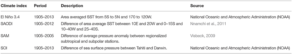
Table 1. Description, period, and source of the Climate Indices.

Methods

Percentile Analysis

In order to analyze long-term changes in the frequency distribution of extreme high and low WLs, we examine the presence of linear trends in the series of annual WL percentiles. This method is widely used to assess changes in extreme WLs because it is less sensitive to outliers than the analysis of annual maxima (Woodworth and Blackman, 2004; Marcos et al., 2009; Haigh et al., 2010; Letetrel et al., 2010; Mudersbach et al., 2013; Wahl and Chambers, 2015). In addition, percentile analysis allows assessing whether changes in extreme WLs are similar to the ones in MSL or whether other factors affect the distribution of extreme WLs.

In a first step, we produce annual series of percentiles, including the 0.05th, 0.5th, 2th, 5th, 10th, 20th, 50th, 80th, 90th, 95th, 98th, 99.5th, and 99.95th percentiles of both WL records for each calendar year (hereafter WL percentile series) with <25% missing values(Haigh et al., 2010; Wahl and Chambers, 2015). The median (50th percentile) can be assumed as a good approximation of MSL, because this percentile is less affected by outliers than the mean. To remove the signal of the MSL we subtract the values of the 50th percentile series from each of the other percentile series, creating another set of annual percentiles series reduced to the medians (hereafter RedM percentile series). In addition, any signal related to vertical land movement is included within the value of the 50th percentile and thus removed by this reduction (Woodworth and Blackman, 2004). However, the contribution of the tide is still present. In order to remove the tidal contribution, we create series of annual tidal percentiles from the predicted WLs. For this purpose, we perform a harmonic analysis for each year separately using the UTide Matlab package (Codiga, 2011), which gives a standard set of 63 tidal constituents with a value of signal-to-noise-ratio of at least two. Based on these tidal constituents, we produce the astronomical WLs of each calendar year of records, and calculate the tidal annual percentiles (0.05th−99.95th) of each calendar year (hereafter Tide percentile series). From each RedM percentile series, we subtract the corresponding Tide percentile series, creating another set of annual percentile series reduced to the median and to the tide (hereafter Residual percentile series). However, the Residual percentiles series still contain the tidal variability related to the perigean (4.4 years) and the nodal cycle (18.6 years) components, which cannot be estimated from annual harmonic analysis. Most of the remaining variability and trends of the Residual percentile series can be attributed to forcings different than MSL and tides, or to non-linear effects caused by the changes in the MSL and tides (Woodworth and Blackman, 2004). We calculate the standard deviation (std) of the Residual percentile series as a measure of the inter-annual variability.

In a next step, we analyze the presence of secular trends in the WL, Tide, and Residual percentile series and the link of the variability of the Residual percentile series to the decadal variability in the regional climate system. Long-term trends are assessed by fitting linear regressions to each annual percentile series of all sets and calculating the significance of the fitted linear model at the 5% significance level. In order to analyze whether extreme WLs are linked to the climate systems of this region, we calculate Spearman's rank correlations, at the 95% confidence level, between the Residual percentiles series and the climate indices El Niño 3.4, SAODI, SOI, and SAM. Spearman is a non-parametric test that measures the strength between two variables using a monotonic function and it does not make any assumption regarding the distribution of the two variables. We produce annual time series of each of these indices by averaging their monthly values per calendar year in order to synchronize them with the Residual percentiles series. We also assess the influence of extreme river runoff by correlating the annual 99.95th percentile series of river discharge from each river tide-gauges (i.e., Túnel subfluvial and Paso de los Libres) with the Residual annual percentile series of Buenos Aires and Mar del Plata.

Tidal Analysis

In order to assess secular changes in tidal levels and the main tidal constituents in Buenos Aires and Mar del Plata, we perform a second harmonic analysis over consecutive periods of 19 years, in order to account for both the perigean and nodal cycle components and reducing the errors of the constituents estimates.

Prior to the harmonic analysis, we de-trend both WL series in order to remove the seasonal variability and long-term trend of the MSL, as well as the vertical land movement signal (Mawdsley et al., 2015). The detrending of the WL series is performed by subtracting the centered 30-days moving average of each hourly WL from both time-series.

Again, we use the UTide Matlab package (Codiga, 2011) to perform a centered 19 years moving harmonic analysis with a lag of 1 year over the detrended time-series. By using the moving harmonic analysis, we shorten our records but we still obtain estimates of the tidal constituents over 90 and 40 years for Buenos Aires and Mar del Plata, respectively. We predict hourly astronomical WLs for each calendar year using the tidal constituents estimated from the harmonic analysis centered on the corresponding year. We calculate the annual mean of different tidal levels of the astronomical WL series of both locations and fit linear regressions to them in order to assess whether the tidal levels show a significant linear trend over the study period.

Buenos Aires and Mar del Plata have a mixed semidiurnal tide, with one of the daily high (low) water peaks being higher (lower) than the other peak (Figure 1). Therefore, the tidal levels selected for the analysis are: higher high water (HHW), lower low water (LLW) and greater diurnal tidal range (GDTR; i.e., difference between the HHW and LLW); lower high water (LHW), higher low water (HLW) and lesser diurnal tidal range (LDTR; i.e., difference between LHW and HLW); mean high water (MHW; mean of HHW and LHW), mean low water (MLW; mean of LLW and HLW) and mean tidal range (MTR; difference between MHW and MLW).

FIGURE 1

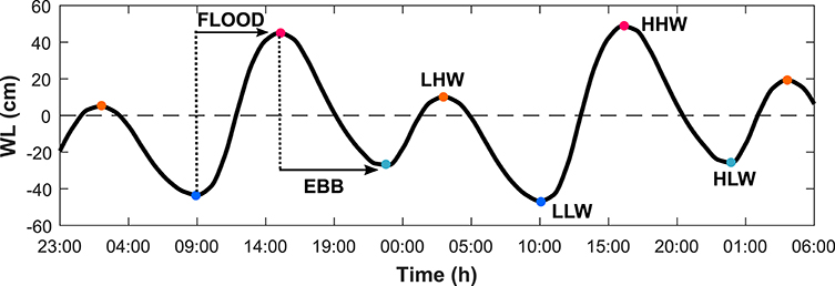
Figure 1. Diagram of the tidal levels and phases of the tidal curve analyzed.

Changes in water depth, e.g., triggered by sea level rise, alter shallow water processes such as tidal wave velocity and energy dissipation by bottom friction, which may change the tidal curve. To assess secular changes in the tidal curve, we analyze the presence of significant long-term linear trends in the annual duration of the ebb and flow phases over the predicted period. We therefore calculate the duration of each flood phase of the astronomical WL series as the time between a low water peak and the following high water peak, as well as the duration of each ebb phase as the time between a high water peak and the successive low water peak. Then, we average both flood and ebb series per each calendar year and fit a linear regression through the flood and ebb annual series as well as to the annual flood/ebb ratio, which is a measure of tidal asymmetry.

Similarly, we assess secular trends in the amplitudes and phases of the main tidal constituents M2, S2, K1, and O1, and the overtide M4 at Buenos Aires and Mar del Plata by fitting linear regressions and analyzing their significance level.

Results

Percentile Analysis

In Buenos Aires, most WL percentile series show significant positive trends ranging between 1.17 to 2.32 mm y⁻¹ (Table 2). Assuming the 50th percentile series to be a good approximation of MSL, we obtain a linear MSL rise of 1.35 mm y⁻¹ over the last century in Buenos Aires. The WL percentile series lower than the median show larger increases than the upper percentiles series, with a difference higher than 1 mm y⁻¹ in some cases (e.g., 0.5th percentile and 99.5th percentile). In Buenos Aires, most of the lower RedM percentile series show a significant positive trend, but none of the upper RedM percentile series. In Mar del Plata, half of the RedM percentile series also show a significant positive trend and we do not find any significant trend in the upper RedM percentile series. Therefore, the lower WL percentile series appears to have risen faster than MSL over the last century, while the upper percentiles series followed a trend similar to MSL. The lower Tide percentile series (i.e., lower than the 50th percentile) also show significant positive trends between 0.27 and 0.51 mm y⁻¹. However, only the Residual 2nd percentile series show a significant positive trend of 0.32 mm y⁻¹.

TABLE 2

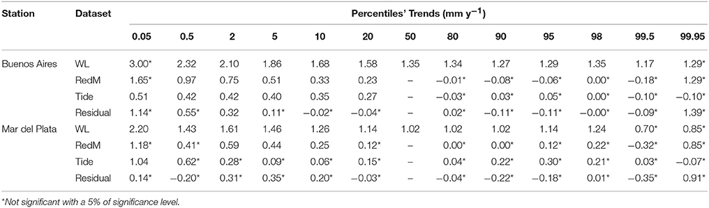
Table 2. Trends (mm y⁻¹) of the WL, RedM, Tide (reduced to their median) and Residual annual percentile series of Buenos Aires and Mar del Plata.

The WL percentile series of Mar del Plata show generally smaller trends than the trends of the WL percentile series of Buenos Aires. We obtain a MSL rise of 1.02 mm y⁻¹ in Mar del Plata over the studied period (1956–2013), which is approximately half of the studied period of Buenos Aires (1905–2013). In Mar del Plata, we also obtain a difference around 1 mm y⁻¹ between the trends of the lower and upper WL percentile series (i.e., below and above the 50th percentile). Only the Tide 0.05th percentile series shows a significant positive trend of 1.04 mm y⁻¹ in Mar del Plata, and none of the Residual percentile series shows a significant trend.

In Figure 2, we can observe that the WL percentile series of Buenos Aires (Figure 2A) also show a greater inter-annual variability than the WL percentile series of Mar del Plata (Figure 2C). Specifically, the Residual 99.95th and 0.05th percentiles series of both locations (Figures 2B,D) show the greatest inter-annual variability, which can be two to three times greater in Buenos Aires (std_0.05 = 62.96 cm and std_99.95 = 31.12 cm) compared to Mar del Plata (std_0.05 = 12.90 cm and std_99.95 = 16.92 cm). In Buenos Aires, we observe that the lowest percentile series has a larger inter-annual variability than the 99.95th percentile. Meanwhile, the inter-annual variability of these percentile series in Mar del Plata is of similar magnitude.

FIGURE 2

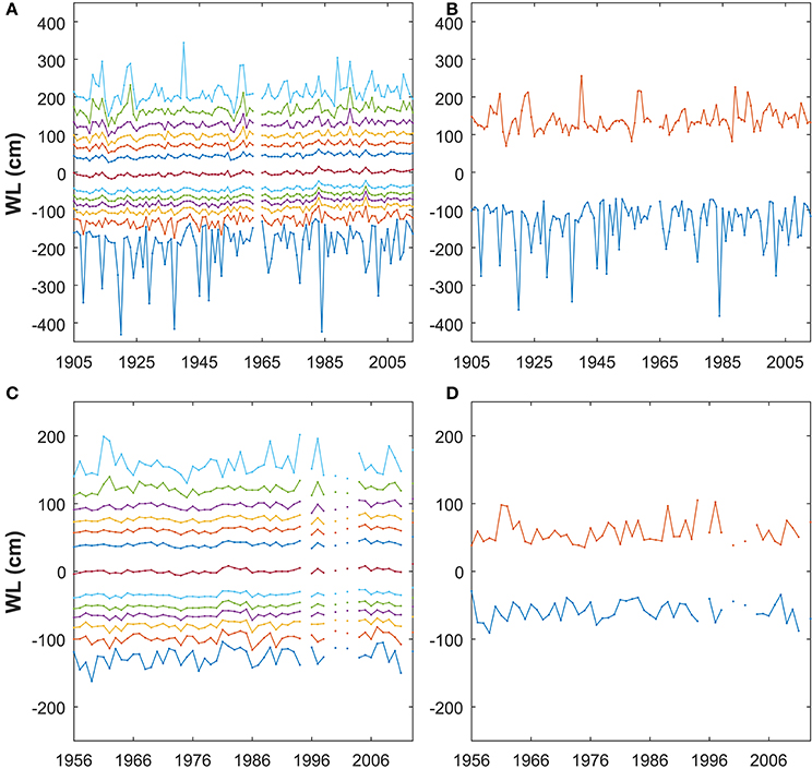
Figure 2. Series of (A) WL percentile series at Buenos Aires (top: 99.5th: bottom: 0.05th), (B) Residual 99.5th (orange) and 0.05th (blue) percentiles series at Buenos Aires, (C) WL percentile series at Mar del Plata (top: 99.5th: bottom: 0.05th), and (D) Residual 99.5th (orange) and 0.05th (blue) percentile series at Mar del Plata.

From the correlation analysis (Figure 3), the Residual 98th and 99.5th percentile series of Buenos Aires show significant correlation with the ENSO indices, positive with El Niño 3.4 and negative with SOI. Meanwhile, in Mar del Plata we observe a negative correlation between the Residual 5th, 10th, and 80th percentile series and El Niño 3.4, and only the 80th percentile series shows a positive correlation with SOI. Regarding the SAODI, we observe a negative correlation with one percentile series in each location, the 98th percentile series in Buenos Aires and the 90th percentile series in Mar del Plata. Similarly, only one Residual percentile series of each location shows a significant correlation to SAM, namely a positive correlation with the 90th percentile series of Buenos Aires and a negative correlation with the 80th percentile series of Mar del Plata. Regarding the correlation with river discharge, we obtain a significant positive correlation between all percentile series above the median, with exception of the 99.95th percentile, in Buenos Aires and the Paraná river discharge (Subfluvial station). However, we only find significant positive correlation between two percentile series (80th and 99.5th percentiles) and the discharge of the Uruguay river (Libres). On the contrary, only the 80th percentile series of Mar del Plata shows a significant negative correlation to the discharge of the Uruguay river.

FIGURE 3

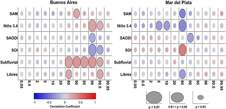
Figure 3. Correlation between climate indices, river runoff and the reduced (to median and tide) annual percentiles of Buenos Aires and Mar del Plata.

Tidal Analysis

In places with a mixed semidiurnal tide, changes in HHW, LLW and thus GDTR may cause greater impacts on flooding, erosion and navigation safety than changes in the other tidal levels, as these levels account for the highest and lowest astronomical WLs. In Figure 4, we present the annual HHW, LLW, and GDTR of Buenos Aires and Mar del Plata over the corresponding study periods. We observe that all tidal levels show an inter-annual variability of several centimeters, but a linear secular trend can also be distinguished in all tidal levels in both locations. As a general pattern, we observe an overall decrease of the annual GDTR driven by an increase of the LLW and a decrease of the HHW. In Buenos Aires, the decrease of the GDTR is more pronounced (0.62 mm y⁻¹) than in Mar del Plata (0.43 mm y⁻¹), and it arises from a large increase of the LLW (0.55 mm y⁻¹) and a low decrease of the HHW (0.08 mm y⁻¹). However, in Buenos Aires we can observe the opposite pattern over some periods e.g., during the first 50 years of records, we observe an increase of the HHW and a decrease of LLW, resulting in an increase of the GDTR of more than 5 cm (Figure 4). In Mar del Plata, these tidal levels show a periodic inter-annual variability of around 2 cm and cycles of 5 years in the HHW and 3 years in the LLW. Besides the inter-annual variability, LLW raised with a rate of 0.15 mm y⁻¹ during the second half of the century, and the HHW decreased 0.28 mm y⁻¹ during the same period (Figure 4).

FIGURE 4

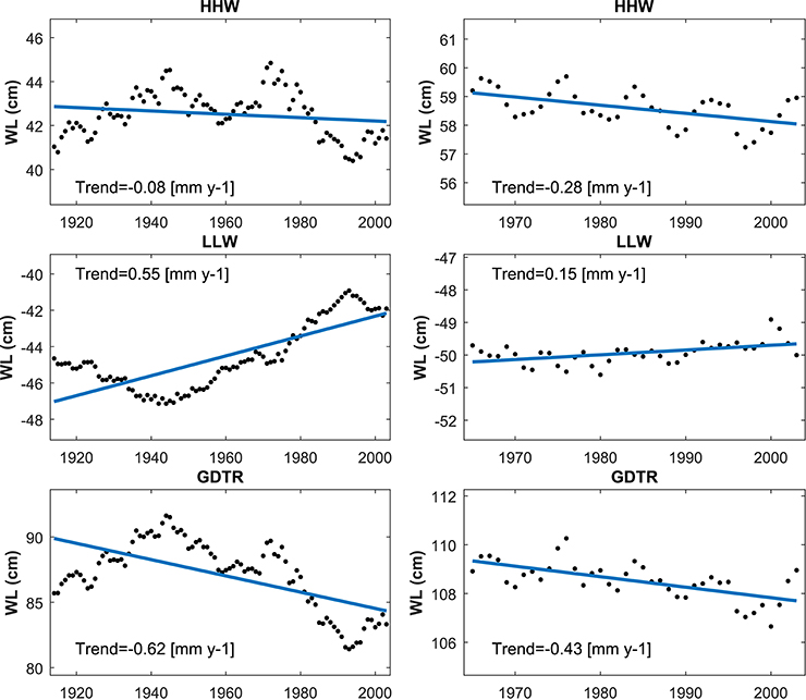
Figure 4. Linear trends of Annual HHW, LLW, and GDTR of Buenos Aires (Left) and Mar del Plata (Right).

The general pattern described for the HHW, LLW and GDTR is also observed in the other tidal levels analyzed (i.e., LHW, HLW, LDTR, HW, LW, and MTR), although they show trends of different magnitude. The results of the other tidal levels can be found in the Supplementary Material (Figures S1, S2).

The differences obtained in the secular trends of the HHW and LLW may produce a change in the tidal curve, thus altering the ebb and flood phases. In shallow water, the asymmetry of the tidal curve is generally characterized by a shorter flood phase with stronger currents and a longer ebb phase with weaker currents (Pugh and Woodworth, 2014). We use the ratio between the annual mean duration of the ebb and flood phases as a measure of the asymmetry of the tidal curve (Figure 5). We observe that both places are flood dominated, as the duration of the flood phase is shorter than the ebb phase, and the asymmetry is greater in Buenos Aires than in Mar del Plata. We find that the asymmetry of the tidal curve shows a small significant increase over the study periods at both locations and also shows an inter-annual variability with a 4 year cyclicity and a magnitude larger than the long-term trend.

FIGURE 5

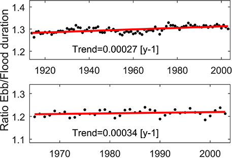
Figure 5. Ratio of the annual mean ebb and flood duration of Buenos Aires (Upper) and Mar del Plata (Lower).

The changes observed in the tidal levels and the asymmetry of the tidal curve have to arise from secular changes in any of the main tidal constituents. Figures 6, 7 show the amplitude and phases of the M2, M4, S2, K1, and O1 constituents obtained from the harmonic analysis over consecutive periods of 19 years for Buenos Aires and Mar del Plata and their secular trends. Almost all tidal constituents show significant trends in both amplitude and phase, with the exception of the O1 amplitude in Buenos Aires. In both locations, the semidiurnal constituents (M2 and S2) show a decrease in the amplitude, while an increase is found in the amplitude of the diurnal constituents (K1 and O1). However, we observe an increase in the phase of both diurnal and semidiurnal tidal constituents, with the exception of the K1 phase in Mar del Plata. In addition, the amplitude and phase of all constituents show an inter-annual variability, which is generally greater in Buenos Aires than in Mar del Plata. For most of the constituents, the inter-annual variability of the amplitude and phase are not showing the same temporal patterns (see e.g., variability of the amplitude and phase of the M2 in Buenos Aires).

FIGURE 6

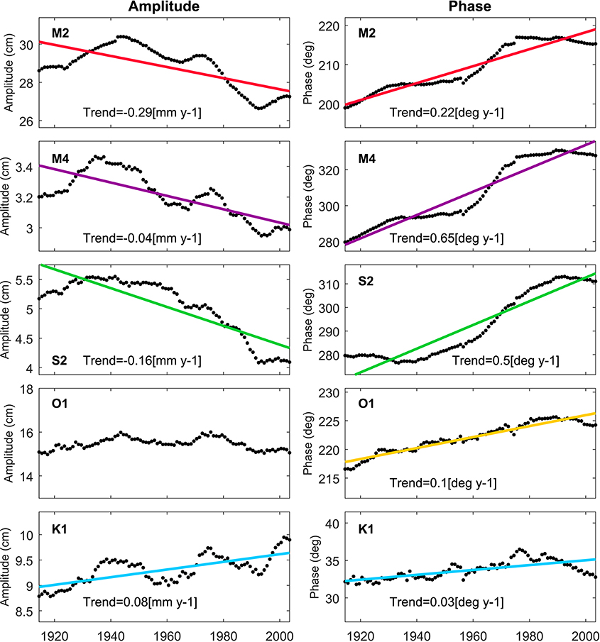
Figure 6. Variability and linear trends of the amplitude and phase of the main tidal constituents of Buenos Aires (only significant trends are shown).

FIGURE 7

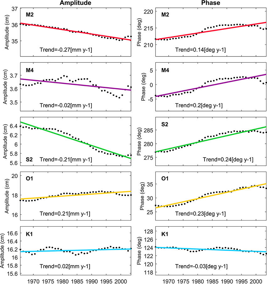
Figure 7. Variability of amplitude and phase of the main tidal constituents of Mar del Plata.

M2 is the tidal constituent with the largest amplitude in both places and the constituent that shows the greatest change in amplitude over the study period. The amplitude of M2 decreased with a similar rate during the last century in Buenos Aires (0.29 mm y⁻¹; Figure 6) as during the last 30 years in Mar del Plata (0.27 mm y⁻¹; Figure 7). However, the M2 amplitude shows some periods of increase in Buenos Aires, but an almost constant decrease in Mar del Plata. The variability observed in the annual GDTR in Buenos Aires (Figure 3) shows a correlation of 0.96 (p = 0) with the pattern of the M2 amplitude, and can thus be explained by the changes in the M2 constituent. In Mar del Plata, the M2 amplitude shows a smaller correlation (0.64 and p = 2.16 · 10⁻⁵) with the GDTR that may be due to the different inter-annual variability observed in both variables (Figure 4).

The S2 constituent, which has a radiational forcing in addition to the gravitational, shows the second more pronounced negative trend in both Buenos Aires (0.16 mm y⁻¹; Figure 6) and Mar del Plata (0.21 mm y⁻¹). We observe that the changes in the amplitude and phase of S2 are simultaneous in both locations, i.e., in periods when the amplitude shows greater decreasing trends, the phase shows a greater increasing trend.

The two diurnal constituents O1 and K1 are the second and third highest constituents in terms of amplitude, at Buenos Aires and Mar del Plata. Opposite to the long-term trends observed in the main semidiurnal constituents, we observe a secular increase in the amplitude of the diurnal constituents at both locations.

The asymmetry of the tidal curve depends on the phase difference between the M2 and M4 constituents (see e.g., Pugh and Woodworth, 2014). In both locations, we find that the phases of both constituents show a positive trend, which is more pronounced for the M4 phase. The difference between the rising rates of the M2 and M4 phases is greater in Buenos Aires (0.22 and 0.65 deg y⁻¹, respectively; Figure 6) than in Mar del Plata (0.14 and 0.2 deg y⁻¹; Figure 7). These results are in line with the greater increase in the tidal asymmetry in Buenos Aires than in Mar del Plata.

Discussion

Long-term trends in WLs can arise from changes in their different components: MSL, tides and non-tidal residuals. Our analysis shows that the WLs of both Buenos Aires and Mar del Plata show significant long-term trends, which originate from MSL rise but also from long-term trends occurring in the tide component. The detailed analysis of the tides corroborates the significant trends observed in the percentile analysis, and shows a long-term decrease of the tidal range in both locations. On the other hand, the residual component shows no significant long-term trends in both locations.

Percentile Analysis

The lower WL percentile series (i.e., lower than the median) of both Buenos Aires and Mar del Plata show larger trends than the upper WL percentile series indicating that the low WLs rose faster than the high WLs and MSL over the study period. Trends in Buenos Aires were higher than those in Mar del Plata. This difference seems to be caused by changes in the tide as we find significant positive trends in the lower RedM and Tide percentile series in Buenos Aires. In Mar del Plata, only three percentile series (2th, 5th, and 10th) show significant trends after their reduction to the median (RedM) and none of the Residual percentile series show a significant trend. However, the Tide 0.05th percentile series presents a significant positive trend, which is 1.04 mm y⁻¹ after subtracting the MSL trend. Therefore, changes in the WLs of Buenos Aires and Mar del Plata are not only caused by an increase in MSL, but also by changes in the tidal component. Although, such changes can affect the generation and propagation of the surge component we do not obtain significant trends in the Residual percentiles series over the study period in both locations. However, Fiore et al. (2009) and D'Onofrio et al. (2008) reported an increase in the magnitude and frequency of the non-tidal residual component of a similar magnitude as MSL rise in Mar del Plata and Buenos Aires, respectively. These two studies assumed the tidal component to be constant over the studied period, thus the changes in the tidal levels that we observe were accounted for as changes in the non-tidal residual component.

We observe that the inter-annual variability of extreme WLs is greater in Buenos Aires compared to Mar del Plata (Figures 2B,D). The location of Buenos Aires, in the inner part of the RdlP estuary results in WLs also being affected by river discharge in addition to the wind-induced set-up. In previous studies on WLs in Buenos Aires, the effect of river runoff on WLs was denied (e.g., D'Onofrio et al., 1999). However, we find a significant correlation between most of the upper WL percentiles series and the annual 99.5th percentile series of the Paraná river discharge, and between two WL percentile series and the annual 99.5th percentile series of the Uruguay river discharge. This indicates that at least extreme river discharge events have a significant effect on the WLs in Buenos Aires.

Extreme river discharge seems to have no effect on the WLs in Mar del Plata as no significant correlation is found between the WL and the river percentile series. An exception is the 80th percentile series, which shows a significant negative correlation to extreme river discharge of the Uruguay river (Paso de los Libres station). It is likely that this significant correlation is due to the meteorological conditions that produce extreme precipitation and alter the WLs in Mar del Plata, and not due to extreme river discharge itself, because the annual mean discharge of this river is lower than the Parana river. Further we also find a significant correlation between this percentile series and the two indices related to ENSO. The opposite can be true for Buenos Aires; we find a significant correlation between two of the upper percentile series and El Niño 3.4 index and SOI that do not necessarily mean a direct effect of the meteorological conditions associated to ENSO on the WLs, but to the higher river runoff associated to this phenomenon (Jaime, 2002). The conditions associated to the SAODI and SAM seem not to be linked to the inter-annual variability of WLs in both locations, because we only find significant correlation of one Residual percentile series of each location to these indices.

Tidal Analysis

We find a long-term trend and inter-annual variability in all tidal levels caused by the changes observed in the amplitude and phase of the main tidal constituents in Buenos Aires and Mar del Plata. The observed secular trends are of similar magnitude as the long-term trends reported in tidal levels of some locations along the northeastern coast of the US and Japan (Mawdsley et al., 2015). However, the magnitude of the trends that we find for the main tidal constituents differs from the ones reported at those locations (Ray, 2009; Rasheed and Chua, 2014).

As a general pattern, we observe a long-term decrease in the tidal range mainly caused by a decrease found in the amplitude of the main semidiurnal constituents M2 and S2. However, it seems that different processes are responsible for the changes observed in Buenos Aires compared to Mar del Plata, as we find substantial differences between the secular trends and inter-annual variability obtained for the tidal levels and constituents between them (e.g., a difference of 0.4 mm y⁻¹ in the trend of LLW; Figure 4). We cannot exclude though that the same factors can have an effect of different magnitude on the tidal levels in Buenos Aires and Mar del Plata.

Changes in the tides have been reported globally with large-scale ocean processes appearing to be the cause (Mawdsley et al., 2015). Nevertheless, different trends in both tidal levels and constituents have been observed in different regions, suggesting that regional and local factors can play an important role (Mawdsley et al., 2015). Several factors have been discussed as responsible for changes in the tidal characteristics observed in other regions. At global scale, these factors are the rise of MSL and changes in ocean stratification, while at local scale morphological changes (i.e., dredging, land reclamation) can also modify tide characteristics (see e.g., Woodworth, 2010; Müller, 2011; Devlin et al., 2014; Hill, 2016).

The rise of the MSL is one of the factors that can produce changes in tidal levels. An increase of the water depth can produce changes in the resonance characteristics of shelfs, in the location of amphidromes and in shallow areas, a reduction of frictional effects that in turn affect overtides such as the M4 as we observe in the RdlP (Pugh and Woodworth, 2014). In Figure 8, we present the 19 years running average of the WLs in Buenos Aires and Mar del Plata and their respective GDTR series showing the co-evolution of the two variables (time series and scatter plot). In Buenos Aires, we observe that MSL and GDTR trends are inversely related in some periods, such as from 1975 to beginning of the 90's, when we see a rapid increase of MSL and simultaneously a rapid decrease of the GDTR occurs. However, we observe a positive correlation of the trends from the beginning of the study period to the mid 40's and since the beginning of the 90's. In Mar del Plata, we can also observe a predominantly negative correlation between the MSL and GDTR, although it is less clear.

FIGURE 8

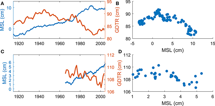
Figure 8. Comparison of the MSL (19 y running average) and the GDTR of (A) Buenos Aires and (C) Mar del Plata; scatter MSL and GDTR of (B) Buenos Aires and (D) Mar del Plata.

None of the above studies comprising the analysis of long-term trends in the tides was able to detect a correlation between the changes observed in the MSL and tides. In addition, studies comprising model simulations of tidal evolution under different SLR scenarios reported that greater rises of water depth are needed in order to produce significant changes in the tides (see e.g., Müller et al., 2011; Pickering et al., 2012, 2017; Carless et al., 2016). Tidal changes obtained from simulations under SLR scenarios depend not only on the SLR scenario and its spatial variability, but also on the stratification scheme and on whether land is allowed to flood (Pickering et al., 2012; Carless et al., 2016). Simulations of high end SLR scenarios (i.e., above 1 m) over the Patagonian shelf performed by Carless et al. (2016) and Luz Clara et al. (2015) showed an increase of the M2 amplitude in the coastal region of Mar del Plata and a decrease of its phase. We observe the opposite pattern during the last 40 years at this location. For Buenos Aires, the global study of Pickering et al. (2017) showed a decrease of the MHW in all SLR scenarios and flooding schemes simulated. According to these contradictory results, the rise of the MSL does not appear to be the only factor producing the changes observed in the tidal levels in Buenos Aires and Mar del Plata.

Changes in stratification and in the thermocline have also been discussed as potential factors causing tidal changes by modifying the coupling of barotropic and internal tides (Colosi and Munk, 2006; Jay, 2009; Müller, 2011; Devlin et al., 2014). The ocean circulation off the study area is characterized by the confluence of the Brazil and Malvinas currents (Palma et al., 2008). The Brazil current brings tropical water of high temperature and salinity, while the Malvinas current transports cold and fresh water from the Antarctic Circumpolar current (Piola et al., 2000; Artana et al., 2016). The different characteristics of these two currents produce a strong thermohaline front with a complex structure (Palma et al., 2008). Besides the seasonal variability of the Brazil/Malvinas confluence region, Combes and Matano (2014) reported a southward trend of this confluence region over the last decade of the twentieth century due to a weakening of the Malvinas current. In addition, the simulations performed by Carless et al. (2016) under an increased stratification scenario over the Patagonian shelf showed a decrease of 15 cm on average of the M2 amplitude along the Argentinian coasts. Therefore, changes in stratification could be responsible for the observed trends in both tidal levels and constituents.

In Buenos Aires, the river discharge into the RdlP is the main factor affecting mixing and tidal propagation into the estuary (Nagy et al., 2008). Luz Clara et al. (2014) reported that the amplitude and phase of the M2 constituent in Buenos Aires show cycles of inter-annual variability that are negatively correlated with the cycles of river runoff, which are positively related to El Niño over the second half of the century. During El Niño, river discharge largely increases and thus increases the downstream currents affecting the upstream progression of the tidal wave (Luz Clara et al., 2014). Therefore, it is likely that the secular trends of both tidal levels and constituents are linked to the increasing river discharge into the RdlP estuary over the last century (Jaime, 2002; Pasquini and Depetris, 2007, 2010), caused by an increase in precipitation and land use changes (Doyle and Barros, 2011). In Figure 9, we present the GDTR of Buenos Aires and the 19-years running average of the Paraná river discharge, which is double the discharge of the Uruguay river and can have a greater impact in the tidal levels in Buenos Aires. We can observe that both series are inversely correlated and the trends of the different periods show a strong negative. The M4 constituent shows a similar inter-annual variability and a negative correlation with the river discharge. The increased bottom friction with higher river discharge modulates the phase and amplitude of the M4 constituent. The secular increase of the river discharge into the RdlP might also be responsible of the observed increase of the asymmetry of the tidal curve, increasing the time of the ebb phase compared to the flood phase.

FIGURE 9

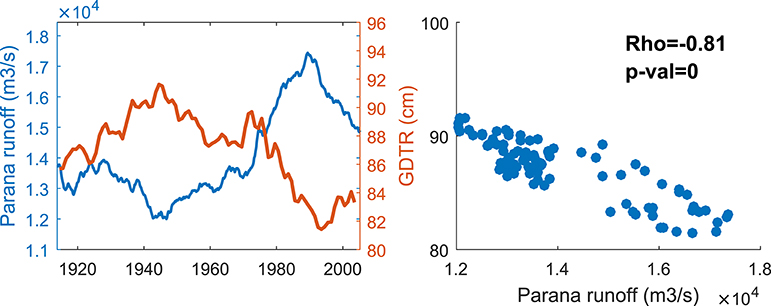
Figure 9. Comparison of the Paraná runoff (19-y running average) and the GDTR of Buenos Aires.

In addition, changes in the atmospheric dynamics and wind-driven circulation may produce changes in the MSL, depth of the mixed layer and sea surface temperature that may affect the tide (Jay, 2009; Müller, 2011; Müller et al., 2014). However, no significant correlation is found between the tidal anomalies in Mar del Plata and any Climate Index. In Buenos Aires, we find significant correlation to ENSO, but it is likely due to the increase of the river discharge in ENSO years (Jaime, 2002).

Local morphological changes caused by e.g., dredging can also produce changes in the tidal characteristics. The tide-gauge of Mar del Plata is located inside the port, which is periodically dredged. In addition, three beaches of Mar del Plata were nourished in 1998, using sand from a sand bank located near the port dikes (Marcomini and Lopez, 2006). Some navigation channels of the RdlP estuary are also periodically dredged and may affect the tidal characteristics of Buenos Aires. In addition, parts of the city of Buenos Aires have been settled on areas gained from the sea, and the vast majority of the land gain (~50 ha) occurred between 1836 to 1998 (Perez Garcia, 2012). These factors can be responsible for periodical or isolated changes of the tidal levels and constituents, but not for the constant trends observed in both tidal levels and constituents at these locations.

Tides control and influence all coastal and biological processes such as sediment transport and coastal ecosystems, and thus secular changes in the tidal characteristics alter those processes. The observed increase of the MLWs in and decrease of MHWs in Buenos Aires may produce a decrease of the intertidal region, thus reducing the area available for intertidal ecosystems. In addition, the vertical growth of the marshes of the RdlP estuary are also affected by changes in tidal range and river discharge (Schuerch et al., 2016). Tide characteristics of Buenos Aires are likely modulated by the river discharge into the RdlP estuary and therefore their effects on marsh development should jointly be taken into account. The observed changes in the tidal levels and constituents as well as the increase in the asymmetry of the tidal curve indicate that also changes in the tidal currents have occurred, which in turn affect sediment transport within the estuary. In the context of flood risk, the observed decrease of the HWs would imply a decrease of the intensity of extreme WLs, in the case that there is no increase of the intensity of storm surges. However, the increase of MLWs leads to an increase of intensity and frequency of storm surge levels coincident with MLWs. Therefore, the observed changes in the tide should be taken into account in trend and extreme analysis of storm surges.

Conclusions

Our analysis shows that low WLs have risen faster than MSL over the last century in Buenos Aires and the last 40 years in Mar del Plata. However, we find no significantly different trend than the MSL trend in those WLs higher than the median. The percentile analysis suggests that the greater trends in the low WLs are mainly caused by trends in the tide component, as we obtain significant trends in the Tide percentiles that can double the trends of the MSL (i.e., 50th percentile). This is confirmed with the results of the running harmonic analysis, which show secular trends in all tidal levels caused by changes in the main tidal constituents (M2, S2, O1, and K1). In both locations, we observe a decrease of the tidal ranges (MTR, GDTR, and LDTR) of 0.5 mm y⁻¹ on average that arises from a decrease of the amplitude of the semidiurnal constituents and an increase of the diurnal constituents, as well as changes in the phases.

Despite trends of the tidal range and tidal constituents being similar in both locations, the drivers do not seem to be the same for Buenos Aires and Mar del Plata. In Buenos Aires, we find a larger positive trend in the LLW than the decrease of the HHW and the changes of these tidal levels show a coherent variability with the variability of the river discharge into the RdlP. Large river discharge reduces the tidal wave propagation into the estuary. Therefore, the large increase of the river discharge over the second half of the twentieth century is likely the reason for the negative trend observed in the tidal range of Buenos Aires. Although, high river discharge may reduce the tidal range and MHWs at Buenos Aires, we also find significant correlation between extreme river discharge and the upper Residual percentiles series. In Mar del Plata, we find a lower increase of the MLWs and a greater decrease of the MHWs than in Buenos Aires, and there is no correlation between the changes in the tides and the river runoff as well as between the Residual percentiles series and extreme river discharge into the RdlP. Therefore, the observed tidal changes are produced by a different factor than in Buenos Aires such as changes in the thermohaline structure of the Brazil/Malvinas confluence region or the rise of the MSL, although for the latter studies have shown that greater increases of the MSL are required to produce significant changes in the tides (Luz Clara et al., 2015; Carless et al., 2016).

Author Contributions

SS-A, MS, AV, and SC: Designed research; SC: Collected the data; SS-A and MS: Processes the data; SS-A, MS, AV, and SC: Analyzed the results; SS-A: Wrote the paper with contributions from MS, AV, and SC. All authors read and approved the final manuscript.

Conflict of Interest Statement

The authors declare that the research was conducted in the absence of any commercial or financial relationships that could be construed as a potential conflict of interest.

Acknowledgments

SS-A and AV were supported by the EU FP7 project RISES-AM (grant agreement 603396). MS was financially supported by the “Deutsche Forschungsgemeinschaft” (DFG) through the Cluster of Excellence 80 “The Future Ocean,” funded within the framework of the Excellence Initiative on behalf of the German federal and state governments, the personal research fellowship of MS (Project Number 272052902) and by the Cambridge Coastal Research Unit (Visiting Scholar Programme). SC work was developed under the research project “Bases para un manejo sustentable de los recursos hídricos en la franja costera arenosa oriental de la Provincia de Buenos Aires” [“Guidelines for the sustainable management of water resources in the eastern coastal sand-dune barrier of the Province of Buenos Aires”] (PICT 2013-2117, ANPCyT, Argentina). We acknowledge the support of the Servicio de Hidrografia Naval (SHN) of Argentina for providing the tide-gauge series. We acknowledge financial support by Land Schleswig-Holstein within the funding programme Open Access Publikationsfonds. We would also like to acknowledge the two reviewers for providing constructive and valuable comments that helped improving the paper.

Supplementary Material

The Supplementary Material for this article can be found online at: https://www.frontiersin.org/articles/10.3389/fmars.2017.00380/full#supplementary-material

References

Artana, C., Ferrari, R., Koenig, Z., Saraceno, M., Piola, A. R., and Provost, C. (2016). Malvinas current variability from argo floats and satellite altimetry. J. Geophys. Res. Oceans 121, 4854–4872. doi: 10.1002/2016JC011889

CrossRef Full Text | Google Scholar

Carless, S. J., Green, J. A. M., Pelling, H. E., and Wilmes, S. B. (2016). Effects of future sea-level rise on tidal processes on the Patagonian shelf. J. Mar. Syst. 163, 113–124. doi: 10.1016/j.jmarsys.2016.07.007

CrossRef Full Text | Google Scholar

Cid, A., Menéndez, M., Castanedo, S., Abascal, A. J., Méndez, F. J., and Medina, R. (2015). Long-term changes in the frequency, intensity and duration of extreme storm surge events in Southern Europe. Clim. Dyn. 46, 1503–1516. doi: 10.1007/s00382-015-2659-1

CrossRef Full Text | Google Scholar

Codiga, D. L. (2011). Unified Tidal Analysis and Prediction Using the UTide Matlab Functions. URI/GSO Technical Report 2011-01, University of Rhode Island. doi: 10.13140/RG.2.1.3761.2008

CrossRef Full Text | Google Scholar

Colosi, J. A., and Munk, W. (2006). Tales of the venerable honolulu tide gauge. J. Phys. Oceanogr. 36, 967–996. doi: 10.1175/JPO2876.1

CrossRef Full Text | Google Scholar

Combes, V., and Matano, R. P. (2014). Trends in the Brazil/Malvinas confluence region. Geophys. Res. Lett. 41, 8971–8977. doi: 10.1002/2014GL062523

CrossRef Full Text | Google Scholar

Devlin, A. T., Jay, D. A., Talke, S. A., and Zaron, E. (2014). Can tidal perturbations associated with sea level variations in the western pacific ocean be used to understand future effects of tidal evolution? Ocean Dyn. 64, 1093–1120. doi: 10.1007/s10236-014-0741-6

CrossRef Full Text | Google Scholar

D'Onofrio, E. E., Fiore, M. M. E., and Pousa, J. L. (2008). Changes in the regime of storm surges at Buenos Aires, Argentina. J. Coast. Res. 1, 260–265. doi: 10.2112/05-0588.1

CrossRef Full Text | Google Scholar

D'Onofrio, E. E., Fiore, M. M. E., and Romero, S. I. (1999). Return periods of extreme water levels estimated for some vulnerable areas of Buenos Aires. Cont. Shelf Res. 19, 1681–1693. doi: 10.1016/S0278-4343(98)00115-0

CrossRef Full Text | Google Scholar

Doyle, M. E., and Barros, V. R. (2011). Attribution of the river flow growth in the plata basin. Int. J. Climatol. 31, 2234–2248. doi: 10.1002/joc.2228

CrossRef Full Text | Google Scholar

Feng, X., Tsimplis, M. N., and Woodworth, P. L. (2015). Nodal variations and long-term changes in the main tides on the coasts of China. J. Geophys. Res. Oceans 120, 1215–1232. doi: 10.1002/2014JC010312

CrossRef Full Text | Google Scholar

Fiore, M. E., D'Onofrio, E. E., Grismeyer, W. H., and Mediavilla, D. G. (2008). El ascenso del nivel del mar en la costa de la provincia de Buenos Aires. Cienc. Hoy 18, 50–57.

Google Scholar

Fiore, M. M. E., D'Onofrio, E. E., Pousa, J. L., Schnack, E. J., and Bértola, G. R. (2009). Storm surges and coastal impacts at Mar Del Plata, Argentina. Cont. Shelf Res. 29, 1643–1649. doi: 10.1016/j.csr.2009.05.004

CrossRef Full Text | Google Scholar

Gillett, N. P., Kell, T. D., and Jones, P. D. (2006). Regional climate impacts of the Southern annular mode. Geophys. Res. Lett. 33:L23704. doi: 10.1029/2006GL027721

CrossRef Full Text | Google Scholar

Haigh, I. D., Wadey, M. P., Wahl, T., Ozsoy, O., Nicholls, R. J., Brown, J. M., et al. (2016). Spatial and temporal analysis of extreme sea level and storm surge events around the coastline of the UK. Sci. Data 3:160107. doi: 10.1038/sdata.2016.107

PubMed Abstract | CrossRef Full Text | Google Scholar

Haigh, I., Nicholls, R., and Wells, N. (2010). Assessing changes in extreme sea levels: application to the English channel, 1900–2006. Cont. Shelf Res. 30, 1042–1055. doi: 10.1016/j.csr.2010.02.002

CrossRef Full Text | Google Scholar

Hill, D. F. (2016). Spatial and temporal variability in tidal range: evidence, causes, and effects. Curr. Clim. Change Rep. 2, 232–241. doi: 10.1007/s40641-016-0044-8

CrossRef Full Text | Google Scholar

Ho, M., Kiem, A. S., and Verdon-Kidd, D. C. (2012). The Southern annular mode: a comparison of indices. Hydrol. Earth Syst. Sci. 16, 967–982. doi: 10.5194/hess-16-967-2012

CrossRef Full Text | Google Scholar

Jaime, P. (2002). “Analisis del regimen hidrologico de los Rios Parana y Uruguay,” in Proteccion Ambiental Del Rio de La Plata Y Su Frente Maritimo: Prevencion Y Control de La Contaminacion Y Restauracion de Habitats, Vol. 53 (Comisión Administradora del Río de la Plata), 160.

Jay, D. A. (2009). Evolution of tidal amplitudes in the Eastern Pacific Ocean. Geophys. Res. Lett. 36, 1–5. doi: 10.1029/2008GL036185

CrossRef Full Text | Google Scholar

Letetrel, C., Marcos, M., Martín Míguez, B., and Woppelmann, G. (2010). Sea level extremes in Marseille (NW Mediterranean) during 1885–2008. Cont. Shelf Res. 30, 1267–1274. doi: 10.1016/j.csr.2010.04.003

CrossRef Full Text | Google Scholar

Luz Clara, M., Simionato, C. G., D'Onofrio, E., and Moreira, D. (2015). Future sea level rise and changes on tides in the Patagonian Continental Shelf. J. Coast. Res. 313, 519–535. doi: 10.2112/JCOASTRES-D-13-00127.1

CrossRef Full Text | Google Scholar

Luz Clara, M., Simionato, C. G., D'Onofrio, E., Fiore, M., and Moreira, D. (2014). Variability of tidal constants in the Río de La Plata estuary associated to the natural cycles of the runoff. Estuar. Coast. Shelf Sci. 148, 85–96. doi: 10.1016/j.ecss.2014.07.002

CrossRef Full Text | Google Scholar

Marcomini, S. C., and López, R. A. (2006). Evolution of a beach nourishment project at Mar Del Plata. J. Coast. Res. 2, 834–837. Available online at: http://www.jstor.org/stable/25741693

Google Scholar

Marcos, M., Calafat, F. M., Berihuete, Á., and Dangendorf, S. (2015). Long-term variations in global sea level extremes. J. Geophys. Res. Oceans 120, 8115–8134. doi: 10.1002/2015JC011173

CrossRef Full Text | Google Scholar

Marcos, M., Tsimplis, M. N., and Shaw, A. G. P. (2009). Sea level extremes in southern Europe. J. Geophys. Res. Ocean. 114:C01007. doi: 10.1029/2008JC004912

CrossRef Full Text | Google Scholar

Mawdsley, R. J., Haigh, I. D., and Wells, N. C. (2015). Global secular changes in different tidal high water, low water and range levels. Earth's Future 3, 66–81. doi: 10.1002/2014EF000282

CrossRef Full Text | Google Scholar

Meccia, V. L., Simionato, C. G., Fiore, M. E., D'Onofrio, E. E., and Dragani, W. C. (2009). Sea surface height variability in the Rio de La Plata estuary from synoptic to inter-annual scales: results of numerical simulations. Estuar. Coast. Shelf Sci. 85, 327–343. doi: 10.1016/j.ecss.2009.08.024

CrossRef Full Text | Google Scholar

Menéndez, M., and Woodworth, P. L. (2010). Changes in extreme high water levels based on a quasi-global tide-gauge data set. J. Geophys. Res. Oceans 115, 1–15. doi: 10.1029/2009JC005997

CrossRef Full Text | Google Scholar

Mudersbach, C., Wahl, T., Haigh, I. D., and Jensen, J. (2013). Trends in high sea levels of German North Sea gauges compared to regional mean sea level changes. Cont. Shelf Res. 65, 111–120. doi: 10.1016/j.csr.2013.06.016

CrossRef Full Text | Google Scholar

Müller, M. (2011). Rapid change in semi-diurnal tides in the North Atlantic since 1980. Geophys. Res. Lett. 38, 1–6. doi: 10.1029/2011GL047312

CrossRef Full Text | Google Scholar

Müller, M., Arbic, B. K., and Mitrovica, J. X. (2011). Secular trends in ocean tides: observations and model results. J. Geophys. Res. Oceans 116, 1–19. doi: 10.1029/2010JC006387

CrossRef Full Text | Google Scholar

Müller, M., Cherniawsky, J. Y., Foreman, M. G. G., and Von Storch, J. S. (2014). Seasonal variation of the M 2 tide. Ocean Dyn. 64, 159–177. doi: 10.1007/s10236-013-0679-0

CrossRef Full Text | Google Scholar

Nagy, G. J., Severov, D. N., Pshennikov, V. A., De los Santos, M., Lagomarsino, J. J., Sans, K., et al. (2008). Rio de La Plata estuarine system: relationship between river flow and frontal variability. Adv. Space Res. 41, 1876–1881. doi: 10.1016/j.asr.2007.11.027

CrossRef Full Text | Google Scholar

Nnamchi, H. C., Li, J., and Anyadike, R. N. C. (2011). Does a dipole mode really exist in the South Atlantic ocean? J. Geophys. Res. Atmos. 116, 1–15. doi: 10.1029/2010JD015579

CrossRef Full Text | Google Scholar

Palma, E. D., Matano, R. P., and Piola, A. R. (2008). A numerical study of the Southwestern Atlantic shelf circulation: stratified ocean response to local and offshore forcing. J. Geophys. Res. Oceans 113, 1–22. doi: 10.1029/2007JC004720

CrossRef Full Text | Google Scholar

Pasquini, A. I., and Depetris, P. J. (2007). Discharge trends and flow dynamics of South American rivers draining the Southern Atlantic seaboard: an overview. J. Hydrol. 333, 385–399. doi: 10.1016/j.jhydrol.2006.09.005

CrossRef Full Text | Google Scholar

Pasquini, A. I., and Depetris, P. J. (2010). ENSO-triggered exceptional flooding in the Paraná River: where is the excess water coming from? J. Hydrol. 383, 186–193. doi: 10.1016/j.jhydrol.2009.12.035

CrossRef Full Text | Google Scholar

Perez Garcia, R. (2012). MESA 2:Rellenos En La Ribera de La Ciudad Metropolitana. In 18° Congreso de Saneamiento Y Medio Ambiente, IV Feria Internacional de Tecnologias Del Medio Ambiente Y En Agua (FITMA), 1–20. Buenos Aires: Fundacion Ciudad.

Pickering, M. D., Wells, N. C., Horsburgh, K. J., and Green, J. A. M. (2012). The impact of future sea-level rise on the European Shelf Tides. Cont. Shelf Res. 35, 1–15. doi: 10.1016/j.csr.2011.11.011

CrossRef Full Text | Google Scholar

Pickering, M. D., Wells, N. C., Horsburgh, K. J., and Green, J. A. M. (2017). The impact of future sea-level rise on the global tides. Cont. Shelf Res. 142, 50–68. doi: 10.1016/j.csr.2017.02.004

CrossRef Full Text | Google Scholar

Piola, A. R., Campos, E. J. D., Möller, O. O., Charo, M., and Martinez, C. (2000). Subtropical shelf front OFF Eastern South America. J. Geophys. Res. Oceans 105, 6565–6578. doi: 10.1029/1999JC000300

CrossRef Full Text | Google Scholar

Pugh, D., and Woodworth, P. (2014). Sea-Level Science: Understanding Tides, Surges, Tsunamis and Mean Sea-Level Changes. Cambridge: Cambridge University Press. doi: 10.1017/CBO9781139235778

CrossRef Full Text | Google Scholar

Rasheed, A. S., and Chua, V. P. (2014). Secular trends in tidal parameters along the coast of Japan. Atmos. Ocean 52, 155–168. doi: 10.1080/07055900.2014.886031

CrossRef Full Text | Google Scholar

Ray, R. D. (2009). Secular changes in the solar semidiurnal tide of the Western North Atlantic Ocean. Geophys. Res. Lett. 36, 1–5. doi: 10.1029/2009GL040217

CrossRef Full Text | Google Scholar

Rhein, M., Rintoul, S. R., Aoki, S., Campos, E., Chambers, D., Feely, R. A., et al. (2013). Climate Change 2013: The Physical Science Basis(Ch3). Climate Change 2013: The Physical Science Basis, Contribution of Working Group I to the Fifth Assessment Report of the Intergovernmental Panel on Climate Change. 62.

Schuerch, M., Scholten, J., Carretero, S., Garcia-Rodriguez, F., Kumbier, K., Baechtiger, M., et al. (2016). The effect of long-term and decadal climate and hydrology variations on estuarine marsh dynamics: an identifying case study from the Río de La Plata. Geomorphology 269, 122–132. doi: 10.1016/j.geomorph.2016.06.029

CrossRef Full Text | Google Scholar

Silvestri, G. E., and Vera, C. S. (2003). Antarctic oscillation signal on precipitation anomalies over Southeastern South America. Geophys. Res. Lett. 30:2115. doi: 10.1029/2003GL018277

CrossRef Full Text | Google Scholar

Silvestri, G., and Vera, C. (2009). Nonstationary impacts of the Southern annular mode on Southern hemisphere climate. J. Clim. 22, 6142–6148. doi: 10.1175/2009JCLI3036.1

CrossRef Full Text | Google Scholar

Visbeck, M. (2009). A station-based southern annular mode index from 1884 to 2005. J. Clim. 22, 940–950. doi: 10.1175/2008JCLI2260.1

CrossRef Full Text | Google Scholar

Wahl, T., and Chambers, D. P. (2015). Evidence for multidecadal variability in US extreme sea level records. J. Geophys. Res. C Oceans 120, 1527–1544. doi: 10.1002/2014JC010443

CrossRef Full Text | Google Scholar

Wahl, T., and Chambers, D. P. (2016). Climate controls multidecadal variability in US extreme sea level records. J. Geophys. Res. Oceans 121, 1274–1290. doi: 10.1002/2015JC011057

CrossRef Full Text | Google Scholar

Wahl, T., Haigh, I. D., Nicholls, R. J., Arns, A., Dangendorf, S., Hinkel, J., et al. (2017). Understanding extreme sea levels for broad-scale coastal impact and adaptation analysis. Nat. Commun. 8:16075. doi: 10.1038/ncomms16075

PubMed Abstract | CrossRef Full Text | Google Scholar

Woodworth, P. L. (2010). A survey of recent changes in the main components of the ocean tide. Cont. Shelf Res. 30, 1680–1691. doi: 10.1016/j.csr.2010.07.002

CrossRef Full Text | Google Scholar

Woodworth, P. L., and Blackman, D. L. (2004). Evidence for systematic changes in extreme high waters since the mid-1970s. J. Clim. 17, 1190–1197. doi: 10.1175/1520-0442(2004)017<1190:EFSCIE>2.0.CO;2

CrossRef Full Text | Google Scholar