Primary Production: Sensitivity to Surface Irradiance and Implications for Archiving Data

1. Introduction

Conventionally, there are two approaches to the measurement of phytoplankton production at sea, both of which require incubation of phytoplankton samples for a finite time (Table 1). One is the so-called in situ method (or its variant, the simulated in situ method) (Lohrenz et al., 1992; Lohrenz, 1993). The object here is to produce data representing the vertical distribution of phytoplankton production through the photic zone. The irradiance that drives the photosynthesis is solar irradiance, attenuated by the sea itself (or by other filters in the case of the simulated in situ method). The estimated vertical profile of phytoplankton photosynthesis can be integrated over depth to calculate production in the water column during the period of the incubation. If the duration of incubation is less than that of the light day, the data may be extrapolated to obtain daily water-column production. The result expresses the daily, autotrophic carbon flux under unit area of sea surface at the place and time from which the sample was drawn, under all prevailing conditions, physical and biological.

TABLE 1

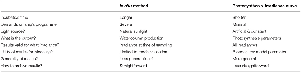
Table 1. Comparison of two approaches (in situ method and photosynthesis-irradiance curve) to measuring primary production of aquatic samples.

The other method is through construction of photosynthesis–light curves. Here, the samples are incubated in artificial light at a sufficient number of irradiance levels that the curve of photosynthetic response can be established, fitted to a standard equation, and the parameters (minimum two for a normal range of irradiances) extracted (Platt and Jassby, 1976). These parameters index the photosynthetic performance of the phytoplankton present at the time and place from which the sample was drawn. The results can be applied in mathematical models to calculate daily watercolumn production (Platt et al., 1977; Sathyendranath and Platt, 1989; Sathyendranath et al., 1989; Morel, 1991; Morel et al., 1996). This serves the same purpose as in situ measurements of primary production, but calculations using the photosynthesis parameters can be tailored for any reasonable time interval, to suit any application. Light-dependent models of primary production are used in remote sensing (Platt and Sathyendranath, 1988; Mélin and Hoepffner, 2004, 2011) and in large-scale simulation models of the marine ecosystem (Laufkötter et al., 2015). The photosynthesis parameters are fundamental bio-optical properties of phytoplankton and have many other applications beyond estimation of water-column production, for example in the calculation of chlorophyll-to-carbon ratio in phytoplankton (Jackson et al., 2017).

The photosynthesis parameters may therefore be considered to contain more information than estimates of in situ production (which they subsume through application of a mathematical model). In the planning of present-day oceanographic expeditions on which phytoplankton production estimates are required, a choice is usually made in favor of the photosynthesis–parameter method (which also imposes fewer restrictions on the movement of the ship than does the in situ method).

The question then arises: How should these data be archived? In the case of in situ production estimates, the picture is clear, except possibly for the time scale involved. The data represent the photosynthetic carbon flux per unit area of the sea surface for the duration of the incubation, perhaps extrapolated to a time scale of 1 day, and can be archived as such. For the (preferred) photosynthesis–response method, the parameters can be archived but they do not in themselves constitute an estimate of phytoplankton production. If they are to be applied to the calculation of daily water-column production, what should be taken as the forcing irradiance? Does it matter? Here, we analyse the sensitivity of daily, water-column production to variable surface irradiance, and discuss the archiving of data on primary production, for example as used in climate studies.

2. Theoretical Background: Non-Spectral-Light, Uniform-Biomass Case

The photosynthesis–irradiance curve relates phytoplankton photosynthesis P to irradiance I. It is convenient, and more general, to work with the normalized photosynthetic rate P^B, where the superscript B indicates normalization to the chlorophyll biomass. Thus,

$\begin{array}{ll}{P}^B(I)=p^B(I;\text{parameters}),& (1)\end{array}$

where p^B is a function to be specified and where various choices are available for the parameter sets. We have shown that, regardless of the parameter set chosen and for any plausible choice of p^B, the various manifestations of Equation (1) can all be recast into a single common form (Platt and Sathyendranath, 1993). The discussion to follow is thus robust against alternative choices of p^B and the parameters. Therefore, with no loss of generality, we shall use as parameters the assimilation number $P_m^B$ and the initial slope α^B of the photosynthesis–irradiance curve. Then,

$\begin{array}{ll}{P}^B(I)=p^B(I;{\alpha }^B,P_m^B).& (2)\end{array}$

In the sea, irradiance is a function of depth z and of time of day t, such that we can write

$\begin{array}{ll}{P}^B(I)=p^B\left(I(z,t);{\alpha }^B,P_m^B\right).& (3)\end{array}$

The desired result is the double integral of Equation (3) over time and depth, which is the daily watercolumn production P_Z,T.

$\begin{array}{ll}{P}_{Z,T}=B{\displaystyle {\int }_0^D}{\displaystyle {\int }_0^{\infty }}{p}^B\left(I(z,t);{\alpha }^B,P_m^B\right)\text{ d}z\text{ d}t,& (4)\end{array}$

where D is the length of day in hours from sunrise and where it is assumed that there is no production outside the interval 0 ≤ t ≤ D. The factor B is taken outside the integral signs because we assume that the chlorophyll biomass is independent of depth. The choice of infinity as the upper limit on the integral over z avoids any ambiguity over depth of the photic zone, without invoking any simplifying assumption. Contributions to the integral from all depths below the photic zone are negligible for all practical purposes.

Under clear-sky conditions, the irradiance at the sea surface I(0, t) can be calculated for any latitude and date according to standard astronomical functions (Bird, 1984; Bird and Riordan, 1986; Sathyendranath and Platt, 1988; Platt et al., 1990). Analytically, the time course of clear-sky irradiance I(t) can be described by a function with two parameters (D and the irradiance at local noon $I_0^m$). Thus, $I(0,t)=I_0^{m}g(t;D)$, where g(t) is a function to be specified. The effect of clouds may be represented through a reduction in the magnitude of $I_0^m$ according to the proportion of the sky covered by clouds.

Given observations of α^B and $P_m^B$ (and a choice of p^B) we can evaluate the double integral of Equation (4) for any station and time. The result will depend upon the magnitude of $I_0^m$. For archival purposes, is it appropriate to use the clear-sky value of $I_0^m$ (which would return the maximum possible value of production under the prevailing conditions at that time and place)? Or is it more appropriate to use the value of $I_0^m$ corresponding to the sky conditions at the station and time (which would return the best value of production for the conditions, but which would lack any generality for other sky conditions)? Would the differences be significant?

To address these issues, we need to look at the derivative of Equation (4) with respect to irradiance. Let us first select $p^B(I)=P_m^B\left(1-exp(-I/I_k)\right)$ as the formulation of the photosynthesis–light curve, where the photoadaptation parameter $I_k=P_m^B/{\alpha }^B$. The ratio I/I_k is a dimensionless irradiance that we designate as I_*. The dimensionless noon irradiance is $I_{*}^m$. We assume a vertically-homogeneous water column so that B(z) = B, and light attenuation can be characterized by a single coefficient K such that I(z) = I(0)exp(−Kz) where the sea surface is at z = 0 and z is positive downwards. Then Equation 4 may be written as

$\begin{array}{ll}{P}_{Z,T}=B{P}_m^B{\displaystyle {\int }_0^D}{\displaystyle {\int }_0^{\infty }}\left(1-exp\left(-I_{*}^{m}g(t)exp(-Kz)\right)\right)\text{ d}z\text{ d}t.& (5)\end{array}$

With a change of variable $x=I_{*}^{m}g(t)exp(-Kz)$, we have

$\begin{array}{ll}{P}_{Z,T}=\frac{B{P}_m^B}{K}{\displaystyle {\int }_0^D}{\displaystyle {\int }_0^{I_{*}^{m}g(t)}}\left(\frac{1-exp\left(-x\right)}{x}\right)\text{ d}x\text{ d}t.& (6)\end{array}$

The inner integral (on x) is a standard form, the entire exponential integral $Ein\left(I_{*}^{m}g(t)\right)$, so that

$\begin{array}{ll}{P}_{Z,T}=\frac{B{P}_m^B}{K}{\displaystyle {\int }_0^D}Ein\left(I_{*}^{m}g(t)\right)\text{ d}t.& (7)\end{array}$

In the specification of the surface irradiance, the dimensionless irradiance at noon $I_{*}^m$ can be considered as a scale factor, with the function g(t) describing the time course of variation through the day. Our immediate interest is on the derivative of P_Z,T with respect to this scale factor $I_{*}^m$,

$\begin{array}{ll}\frac{\text{d}{P}_{Z,T}}{\text{d}{I}_{*}^m}=\frac{B{P}_m^B}{K}{\displaystyle {\int }_0^D}\frac{\text{d}}{\text{d}{I}_{*}^m}Ein\left(I_{*}^{m}g(t)\right)\text{ d}t.& (8)\end{array}$

By virtue of the definition of the function Ein(.) as an integral, the differentiation returns the integrand of the definition:

$\begin{array}{ll}\frac{\text{d}{P}_{Z,T}}{\text{d}{I}_{*}^m}=\frac{B{P}_m^B}{K}{\displaystyle {\int }_0^D}g\left(t\right)\left(\frac{1-exp\left(-I_{*}^{m}g\left(t\right)\right)}{I_{*}^{m}g\left(t\right)}\right)\text{ d}t.& (9)\end{array}$

The functions g(t) in numerator and denominator cancel to give the simple result

$\begin{array}{ll}\frac{d{P}_{Z,T}}{d{I}_{*}^m}=\frac{B{P}_m^B}{K{I}_{*}^m}{\displaystyle {\int }_0^D\left(1-\exp (-I_{*}^{m}g(t))\right)} \text{d}t.& (10)\end{array}$

The choice of function g(t) = 1 − (1 − 2t/D)² gives a good representation of the time course of surface irradiance through the day. With this choice, and with the substitution θ = πt/D, Equation 10 becomes

$\begin{array}{ll}\frac{\text{d}{P}_{Z,T}}{\text{d}{I}_{*}^m}=\frac{B{P}_m^B}{K{I}_{*}^m}\frac{D}{\pi }{\displaystyle {\int }_0^{\pi }}\left(1-exp\left(-I_{*}^m\left[1-{(1-2\theta /\pi )}^2\right]\right)\right)\text{ d}\theta .& (11)\end{array}$

Given the symmetry of g(θ) about θ = π/2, we can express Equation (11) as

$\begin{array}{ll}\frac{\text{d}{P}_{Z,T}}{\text{d}{I}_{*}^m}=\frac{B{P}_m^B}{K{I}_{*}^m}\frac{D}{\pi }\left\{\pi -2{\displaystyle {\int }_0^{\pi /2}}exp\left(-I_{*}^m\left[1-{\left(1-2\theta /\pi \right)}^2\right]\right)\text{ d}\theta \right\}.& (12)\end{array}$

At this point it is convenient to make the substitution $s=\sqrt{I_{*}^m}(1-2\theta /\pi )$. Then,

$\begin{array}{ll}\frac{\text{d}{P}_{Z,T}}{\text{d}{I}_{*}^m}=\frac{B{P}_m^B}{K{I}_{*}^m}\frac{D}{\pi }\left\{\pi -\frac{\pi e^{-I_{*}^m}}{\sqrt{I_{*}^m}}{\displaystyle {\int }_0^{\sqrt{I_{*}^m}}}{e}^{s^2}\text{d}s\right\}.& (13)\end{array}$

Using the definition of Dawson's integral:

$\begin{array}{ll}Daw\left(x\right)=e^{-x^2}{\displaystyle {\int }_0^x}{e}^{s^2}\text{d}s& (14)\end{array}$

with $x=\sqrt{I_{*}^m}$, we see that Equation (13) can be written as

$\begin{array}{ll}\frac{\text{d}{P}_{Z,T}}{\text{d}{I}_{*}^m}=\frac{B{P}_m^{B}D}{K{I}_{*}^m}\left\{1-\frac{1}{\sqrt{I_{*}^m}}Daw\left(\sqrt{I_{*}^m}\right)\right\}.& (15)\end{array}$

This form is convenient because there exist robust numerical forms for computing Daw(x).

We want to assess the sensitivity of the daily production estimates to changes (errors) in the surface irradiance $I_0^m$. Noting that $\text{d}{I}_0^m=I_k\text{d}{I}_{*}^m$, we can rewrite Equation (15) as

$\begin{array}{ll}\frac{\text{d}{P}_{Z,T}}{\text{d}{I}_0^m}=\frac{B{P}_m^{B}D}{K{I}_0^m}\left\{1-\frac{1}{\sqrt{I_{*}^m}}Daw\left(\sqrt{I_{*}^m}\right)\right\}.& (16)\end{array}$

It was shown in Platt and Sathyendranath (1993) that all solutions to Equation (4) can be written in the canonical form

$\begin{array}{ll}{P}_{Z,T}=Af\left(I_{*}^m\right),& (17)\end{array}$

where $A=B{P}_m^{B}D/K$ is a scale factor with dimensions of daily production, and $f(I_{*}^m)$ is a (known) function of the dimensionless irradiance whose particular form depends on the choice of the photosynthesis-light curve. Dividing both sides of Equation (16) by $Af(I_{*}^m)$, we obtain

$\begin{array}{ll}\left(\frac{d{P}_{Z,T}}{P_{Z,T}}\right)/\left(\frac{d{I}_0^m}{I_0^m}\right)=\frac{1}{f\left(I_{*}^m\right)}\left\{1-\frac{1}{\sqrt{I_{*}^m}}\text{Daw}\left(\sqrt{I_{*}^m}\right)\right\}.& (18)\end{array}$

Here, we can see that the relative change in daily primary production for a given relative change in surface irradiance depends only on a function of the scaled irradiance.

3. Estimating Daily, Water-Column Production

In the previous section, we found an expression for the sensitivity of primary production to variations in surface irradiance, of an idealized water column chosen for mathematical tractability. We next consider the detailed calculation of primary production in operational mode and the sensitivity of the results to changes in the surface irradiance.

Various procedures exist for estimating daily, water-column production by phytoplankton, given information on the two photosynthesis parameters $P_m^B$ and α^B (Platt et al., 1977, 1990, 2008; Platt and Sathyendranath, 1988, 1993). All require an estimate of surface irradiance. Briefly, the differences among them depend mainly on whether a depth-independent biomass profile is assumed and on whether the (known) wavelength dependence of light penetration and photosynthetic response is included or suppressed. A depth-independent, spectrally-neutral treatment provides a frame of reference (Sathyendranath et al., 1989; Platt and Sathyendranath, 1991); it has the canonical solution given in Equation (17).

At the other extreme, a wavelength-dependent and non-uniform biomass treatment has no analytic solution (although Equation 17 remains a reliable guide) and must be integrated numerically (Sathyendranath et al., 1989; Platt and Sathyendranath, 1991). This is the preferred calculation, and its reliability has been demonstrated (Platt and Sathyendranath, 1988). Applications of the various models have been compared (Platt et al., 1991; Kyewalyanga et al., 1992). In the most detailed models, the angular distribution of the irradiance is included (Platt and Sathyendranath, 1988; Sathyendranath and Platt, 1989; Sathyendranath et al., 1989), the light field being separated into its direct and diffuse components. The direct component is affected much more strongly by the presence of clouds, and the diffuse component (which may be one half of the total) will still be available for photosynthesis even under 100% cloud cover. For this reason, separation of the forcing irradiance into direct and diffuse components is a key step in addressing the sensitivity of water column production to variations in cloud cover.

For the calculations presented here, we use a spectral- and angular-distribution-resolving primary-production model (Platt and Sathyendranath, 1988; Longhurst et al., 1995; Platt et al., 1995; Sathyendranath et al., 1995), forced by remotely-sensed chlorophyll and light data, and information derived from ship-based in situ measurements on phytoplankton physiology and vertical biomass profile parameters. These model parameters were organized according to season and ecological province, as in Longhurst et al. (1995). Photophysiological parameter ($P_B^m$ and α^B) values for defined biogeochemical provinces were taken from the work of Mélin and Hoepffner (2004). The vertical structure of the phytoplankton biomass profile was described by three parameters: the depth of maximum chlorophyll concentration (Z_m), the thickness of the subsurface peak in chlorophyll concentration (σ) and the ratio of the peak chlorophyll concentration to the background chlorophyll concentration (ρ), also provided on a provincial basis following Mélin and Hoepffner (2011). To provide a smooth transition of parameter estimates across province boundaries, a smoothing filter was applied to the province values of Mélin and Hoepffner (2004) where values at a given pixel were averaged from a 30 × 30 pixel box, with a pixel size of 9 km, centered on the pixel of interest.

The chlorophyll profile parameters were used in conjunction with the remotely-sensed chlorophyll data from the OC-CCI v1.0 products (Sathyendranath et al., 2016), to create chlorophyll profiles for each 9 km pixel. Average sea-surface irradiance (Photosynthetically-Active Radiation) for May 2011 was taken from three data sources. The first PAR data source was the NASA MODIS PAR product (OBPG, 2014b); the second data source was the NASA MERIS PAR product (OBPG, 2014a); the third source was a new ESA processing of MERIS as documented in the Algorithm Theoretical Baseline Document (ATBD) for the PAR and Primary Production (PPP) SEOM project.

In each of the three cases, the remotely-sensed PAR was used to scale the results of a spectral clear-sky model to provide spectrally-resolved irradiance for input to the primary production model. The propagation of spectral light to various depths in the water column accounted for attenuation by water, phytoplankton and other colored and scattering substances, assuming all optical properties were related to chlorophyll concentration (open-ocean conditions). The profile of light was then combined with the vertical profile of chlorophyll and photosynthetic parameters to obtain estimates of depth-resolved primary production. The calculations were repeated for 12 time steps during half the day length. The results were then integrated over time and depth to yield total primary production per day and per unit area.

4. Sensitivity of P_Z,T to Variations in Surface Irradiance

For the non-spectral approximation, with vertically-uniform biomass profile, the sensitivity of daily, water-column production is given by Equation (18), shown in Figure 1. The spectral analog, calculated by numerical integration for the case of uniform biomass, is shown in Figure 2. The spectral results lie in the same range as that for the non-spectral case, varying slightly according to the chlorophyll concentration. The differences are greater for higher values of chlorophyll and higher values of normalized irradiance. We see that, in both spectral and non-spectral calculations, sensitivity is high and approaches one (corresponding to the case when relative change in primary production is the same as the relative change in surface irradiance) when the dimensionless noon-time irradiance approaches zero. As the scaled noon-time irradiance increases, the sensitivity decreases, reaching values less than 0.5 for $I_{*}^m$ greater than 10. For the spectral model, there is an additional dependence of the answer on chlorophyll concentration: the sensitivity is less than that of the non-spectral case at low $I_{*}^m$, but the opposite holds for high $I_{*}^m$ values. The additional dependence of the results on chlorophyll concentration arises from the effect of phytoplankton absorption on the spectral quality of the underwater light field, which is not taken into account in the non-spectral model. When phytoplankton absorption increases (high-chlorophyll conditions), the water turns progressively green, and less suitable for phytoplankton absorption, introducing a decrease in light available for photosynthesis. The effect on primary production is equivalent to decreasing $I_{*}^m$ in a non-spectral model. For chlorophyll concentration less than 1 mg m⁻³, which would be typical of most open-ocean waters, the spectral and non-spectral models yield results that are quite close to each other, such that the analytical solution may be taken to be a reasonable guide to realistic open-ocean conditions.

FIGURE 1

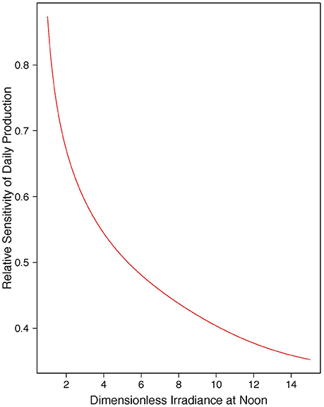
Figure 1. Relative sensitivity of daily, watercolumn primary production (P_Z,T) to changes in dimensionless irradiance at noon ($I_{*}^m$), non-spectral solution, Equation (18).

FIGURE 2

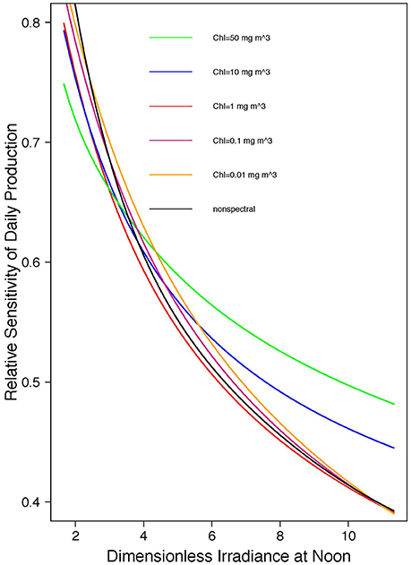
Figure 2. Relative sensitivity of daily, watercolumn primary production (P_Z,T) to changes in dimensionless irradiance at noon ($I_{*}^m$), spectral results by numerical integration for different chlorophyll concentrations. Non-spectral result also shown, for comparison.

In global-scale computations, in addition to the spectral effects, we also have to explore the effect of vertical structure in chlorophyll concentration. We have estimated the global-scale effect of variations in surface irradiance as follows. We selected the month of May, 2011 to illustrate the results. First, we calculated primary production using a detailed, spectral model integrated numerically (Figure 3C), forced by the typical irradiance at each pixel for the month concerned (Figure 3A), using a spectral model, and with the photosynthesis parameters and chlorophyll profile parameters assigned according to provinces and season, as noted earlier. Then, we repeated the calculation (Figure 3B), but with irradiance only one half of that in the previous calculation (Figure 3D). The difference between values of P_Z,T calculated for the two irradiances is a measure of the sensitivity of the daily, water-column production to changes in surface light (Figure 3E) and the relative sensitivity (change in production normalized to change in surface irradiance) is shown in Figure 3F.

FIGURE 3

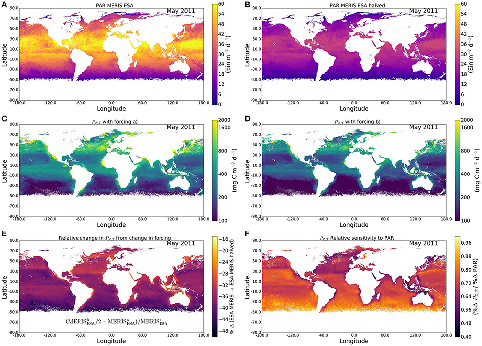
Figure 3. Effect on daily, watercolumn production of a 50% reduction in surface irradiance for May 2011. (A) Surface PAR field before reduction; (B) Surface PAR field after reduction; (C) daily production before reduction of surface light; (D) daily production after reduction of surface light; (E) relative change in primary production following reduction of surface light; and (F) relative change in primary production following reduction of surface light, normalized to the relative change in surface light.

The results, which vary with region (especially with latitude) are not symmetrical about the equator: they represent Spring in the northern hemisphere, but Winter in the southern hemisphere, with corresponding changes to the surface light field (Figure 3A). The results also reflect the regional assignment of photosynthesis parameters. The relative reduction in daily, water-column production lies generally in the range from 30 to 40%, consequent on halving the surface irradiance (Figure 3E). The sensitivity of daily production to changes in surface irradiance is typically in the range from 60 to 80% (Figures 3F, 4), showing that the relative change in primary production is almost always less than the relative change in incoming solar radiation. The relative effect is stronger in areas with low surface irradiance, consistent with the diagnosis of the analytical solution.

FIGURE 4

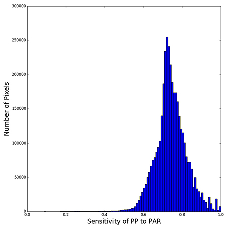
Figure 4. Histogram of relative change in daily production for a 50% reduction in surface irradiance on all sea pixels in Figure 3E.

Systematic errors may be introduced into the calculation of primary production through the choice of the surface field of photosynthetically-active radiation (PAR). We have examined this possibility by comparing the results arising from use of MERIS (Figures 5A,C) and MODIS (Figure 5E) fields of PAR (Figures 5B,D,F). We find that the differences in surface PAR between the two data streams are usually in the range from 5 to 20% (Figure 5E), implying a potential systematic error in primary production of some 15% or less arising from the choice of PAR field. Though these differences may be small, they are systematic; their effect could be significant in studies associated with climate change: when results from multiple sensors are merged to create a long time series, differences between PAR data from individual sensors may lead to an erroneous conclusion on trends in primary production, which is to be avoided.

FIGURE 5

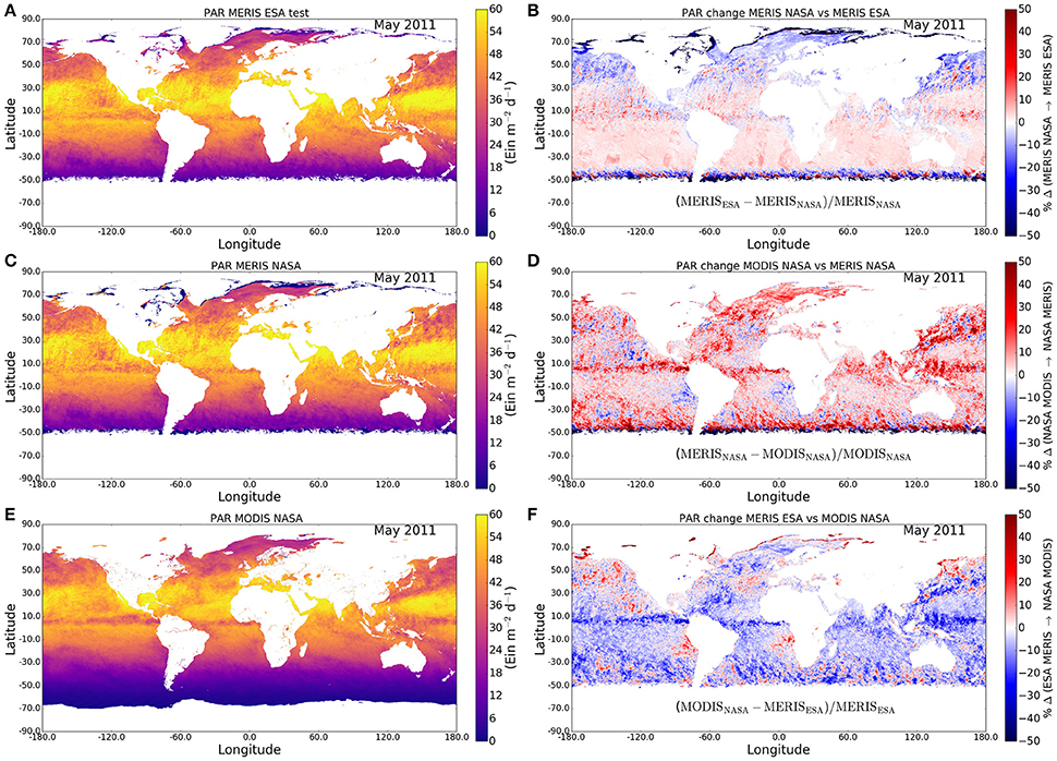
Figure 5. Systematic differences in surface PAR arising from choice of data stream, exemplified by difference between MERIS and MODIS streams for May 2011. (A) PAR field from MERIS using ESA protocol (test product); (C) PAR field from MERIS using NASA product; (E) PAR field from MODIS Aqua using NASA product; the differences between the products are shown in (B,D,F).

5. Discussion

In this paper, we have examined the sensitivity of modeled primary production to changes in the solar radiation available at the sea surface. Using an analytical solution derived for a non-spectral model assuming uniform chlorophyll concentration in the water column, using a spectral model with uniform chlorophyll concentration, and finally using a spectral model with non-uniform chlorophyll profile, we have demonstrated that the relative changes in primary production are likely to be always less than the relative change in surface irradiance. The effect of surface light on primary production decreases as the scaled surface irradiance increases. In the non-spectral model, the only parameter that affects the sensitivity is the photoadaptation parameter I_k. In the spectral model, the chlorophyll concentration has an additional modulating effect on the sensitivity.

In the light of these results, how might we enhance the management of primary production data? Given an archived set of photosynthesis-light parameters what is the most useful information that could be archived about the corresponding phytoplankton production? We suggest the following: First, calculate the phytoplankton production under the climatological value of the clear sky irradiance for the day number and latitude concerned. This represents the maximum phytoplankton production that could be achieved with the given photosynthesis parameters on that day of the year at that latitude. Next, calculate the production under 100% cloud cover, representing the minimum production that could be achieved under the prevailing conditions. These two calculations would establish the range of possible values of phytoplankton production expected at the relevant time and place under most of the possible values of surface irradiance. In fact, because the surface irradiance has both diffuse and direct components, 100% cloud cover will correspond to a reduction in $I_0^m$ of nominally 50% (loss of direct component); all light reaching the sea surface will be in the diffuse component. The effect on daily production of halving the surface irradiance varies with region and season. Taking 50% as a rough estimate of the scope for variation in surface irradiance at a given time and place, we have shown that the implied relative variation in daily, water column is roughly 30–40%. The relative sensitivity, as given by Equation (18), will be independent of the magnitude chosen for the reduction in surface irradiance. A further systematic difference of about 15% may arise from the choice of data source for the surface irradiance field, indicating the value of improving the satellite-derived estimates of PAR.

The most useful particular value of phytoplankton production would be that at the climatologically-averaged value of surface irradiance at the time and place concerned. This average would take into account the effect of latitude on day length and also the local effect of cloud cover. As an example, for the Northwest Atlantic Ocean, we have developed from the SeaWiFS irradiance an empirical function that yields the climatological total daily irradiance as a function of latitude and day number (Platt et al., 2009). If longitudinal differences in cloud cover are to be taken into account, one could use the climatological data on cloud cover to estimate the relevant irradiance.

Paradoxically, the estimate of phytoplankton production made with the irradiance measured at the same time as the parameters themselves were measured (if available) is often the least useful (lowest generality) of all the estimates. Of course, the matter depends on the question being addressed. If the goal is to close a local carbon budget or a local energy budget over a short time period including the day of measurement, then the estimate of phytoplankton production made with the actual irradiance for that particular day would be the one to choose.

However, we expect that most applications of the archived data would be more general than this. In such cases, we would seek estimates of phytoplankton production that were suitably general, and the options we have indicated above would probably be preferred.

The light field in the sea is the resultant of a complex and reciprocal interplay between physics and biology (Figure 6). The effect on daily, water-column production consequent on changes in irradiance at the sea surface depends, at least, on the processes shown in Figure 6. A guide to the scale of the effect (not accounting for spectral dependence) is provided by Equation (18). Spectral effects can be parameterized as a function of chlorophyll concentration (Figure 2).

FIGURE 6

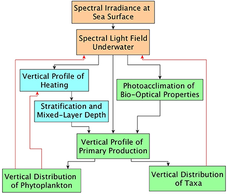
Figure 6. Schematic showing principal factors affecting spectral irradiance field under water, and consequences for watercolumn production. The underwater light field is the resultant of a complex and reciprocal interplay between physics and biology.

Author Contributions

TP, SS, and HB originated the work and organized assembly of the global data bases. GW and TP developed the theoretical background. TJ and SSP made most of the calculations. TP wrote the first draft of the paper. All authors contributed to revision of the paper.

Funding

Funding for this work was provided through the European Space Agency (ESA), contracts 4000113690/15/I-LG and 4000110968/14/I-BG; and through the National Centre for Earth Observation (NCEO), grant PR140015. Additional support from the Simons Foundation CBIOMES project is acknowledged.

Conflict of Interest Statement

The authors declare that the research was conducted in the absence of any commercial or financial relationships that could be construed as a potential conflict of interest.

Acknowledgments

This work is a contribution to the “PAR for Primary Production” Project and the “Photosynthesis Parameters from Space” Project of the European Space Agency. Support from the Jawaharlal Nehru Science Fellowship to TP is gratefully acknowledged. Additional support was received from the National Centre for Earth Observation (NCEO) of the Natural Environment Research Council of UK. The authors thank the two reviewers for their helpful comments.

References

Bird, R. E. (1984). A simple, solar spectral model for direct-normal and diffuse horizontal irradiance. Sol. Energy 32, 461–471. doi: 10.1016/0038-092X(84)90260-3

CrossRef Full Text | Google Scholar

Bird, R. E., and Riordan, C. J. (1986). Simple simple solar spectral model for direct and diffuse irradiance on horizontal and tilted planes at the earth's surface for cloudless atmospheres. J. Clim. Appl. Meteorol. 25, 87–97.

Google Scholar

Jackson, T., Sathyendranath, S., and Platt, T. (2017). An exact solution for modelling photoacclimation of the carbon-to-chlorophyll ratio in phytoplankton. Front. Mar. Sci. 4:283. doi: 10.3389/fmars.2017.00283

CrossRef Full Text | Google Scholar

Kyewalyanga, M., Platt, T., and Sathyendranath, S. (1992). Ocean primary production calculated by spectral and broad-band models. Mar. Ecol. Prog. Ser. 85, 171–185. doi: 10.3354/meps085171

CrossRef Full Text | Google Scholar

Laufkötter, C., Vogt, M., Gruber, N., Aita-Noguchi, M., Aumont, O., Bopp, L., et al. (2015). Drivers and uncertainties of future global marine primary production in marine ecosystem models. Biogeosciences 12, 6955–6984. doi: 10.5194/bg-12-6955-2015

CrossRef Full Text | Google Scholar

Lohrenz, S. E. (1993). Estimation of primary production by the simulated in situ method. ICES Mar. Sei. Symp. 197, 159–171.

Google Scholar

Lohrenz, S. E., Wiesenburg, D. A., Rein, C. R., Arnone, R. A., Taylor, C. D., Knauer, G. A., et al. (1992). A comparison of in situ and simulated in situ methods for estimating oceanic primary production. J. Plankt. Res. 14, 201–221. doi: 10.1093/plankt/14.2.201

CrossRef Full Text | Google Scholar

Longhurst, A. R., Sathyendranath, S., Platt, T., and Caverhill, C. M. (1995). An estimate of global primary production in the ocean from satellite radiometer data. J. Plankton Res. 17, 1245–1271. doi: 10.1093/plankt/17.6.1245

CrossRef Full Text | Google Scholar

Mélin, F., and Hoepffner, N. (2004). Global Marine Primary Production: A Satellite View. Ispra: Institute for Environment and Sustainability.

Mélin, F., and Hoepffner, N. (2011). Monitoring Phytoplankton Productivity from Satellite, Chap. 6. Dartmouth, NS: EU PRESPO and IOCCG.

Google Scholar

Morel, A. (1991). Light and marine photosynthesis: a spectral model with geochemical and climatological implications. Prog. Oceanogr. 26, 263–306. doi: 10.1016/0079-6611(91)90004-6

CrossRef Full Text | Google Scholar

Morel, A., Antoine, D., Babin, M., and Dandonneau, Y. (1996). Measured and modeled primary production in the northeast atlantic (eumeli jgofs program): the impact of natural variations in photosynthetic parameters on model predictive skill. Deep Sea Res. I 43, 1273–1304. doi: 10.1016/0967-0637(96)00059-3

CrossRef Full Text | Google Scholar

OBPG (2014a). Medium Resolution Imaging Spectrometer (MERIS) Photosynthetically Available Radiation Data, 2014 Reprocessing. NASA OB.DAAC. Greenbelt, MD: NASA Goddard Space Flight Center, Ocean Ecology Laboratory, Ocean Biology Processing Group. doi: 10.5067/ENVISAT/MERIS/L3B/PAR/2014

CrossRef Full Text

OBPG (2014b). Moderate-resolution Imaging Spectroradiometer (MODIS) Aqua Photosynthetically Available Radiation Data; 2014 Reprocessing. NASA OB.DAAC. Greenbelt, MD: NASA Goddard Space Flight Center, Ocean Ecology Laboratory, Ocean Biology Processing Group. doi: 10.5067/AQUA/MODIS/L3B/PAR/2014

CrossRef Full Text

Platt, T., Caverhill, C., and Sathyendranath, S. (1991). Basin-scale estimates of oceanic primary production by remote sensing: the north atlantic. J. Geophys. Res. 96, 15147–15159. doi: 10.1029/91JC01118

CrossRef Full Text | Google Scholar

Platt, T., Denman, K., and Jassby, A. (1977). “Modeling the productivity of phytoplankton,” in The Sea: Ideas and Observations on Progress in the Study of the Seas, Vol. VI, ed E. D. Goldberg (New York, NY: John Wiley), 807–856.

Platt, T., and Jassby, A. D. (1976). The relationship between photosynthesis and light for natural assemblages of coastal marine phytoplankton. J. Phycol. 12, 421–430. doi: 10.1111/j.1529-8817.1976.tb02866.x

CrossRef Full Text | Google Scholar

Platt, T., and Sathyendranath, S. (1988). Oceanic primary production: estimation by remote sensing at local and regional scales. Science 241, 1613–1620. doi: 10.1126/science.241.4873.1613

PubMed Abstract | CrossRef Full Text | Google Scholar

Platt, T., and Sathyendranath, S. (1991). Biological production models as elements of coupled, atmosphere-ocean models for climate research. J. Geophys. Res. 96, 2585–2592. doi: 10.1029/90JC02305

CrossRef Full Text | Google Scholar

Platt, T., and Sathyendranath, S. (1993). Estimators of primary production for interpretation of remotely sensed data on ocean color. J. Geophys. Res. 98, 14561–14576. doi: 10.1029/93JC01001

CrossRef Full Text | Google Scholar

Platt, T., Sathyendranath, S., Forget, M.-H., White, G. N. III, Caverhill, C., Bouman, H., et al. (2008). Operational mode estimation of primary production at large geographical scales. Remote Sens. Environ. 112, 3437–3448. doi: 10.1016/j.rse.2007.11.018

CrossRef Full Text | Google Scholar

Platt, T., Sathyendranath, S., and Longhurst, A. (1995). Remote sensing of primary production in the ocean: promise and fulfilment. Philos. Trans. R. Soc. Lond. B 348, 191–202. doi: 10.1098/rstb.1995.0061

CrossRef Full Text

Platt, T., Sathyendranath, S., and Ravindran, P. (1990). Primary production by phytoplankton: analytic solutions for daily rates per unit area of water surface. Proc. R. Soc. Lond. Ser. B 241, 101–111. doi: 10.1098/rspb.1990.0072

CrossRef Full Text | Google Scholar

Platt, T., Sathyendranath, S., White, G. N. III, Fuentes-Yaco, C., Zhai, L., Devred, E., et al. (2009). Diagnostic properties of phytoplankton time series from remote sensing. Estuar. Coasts 32, 428–439. doi: 10.1007/s12237-009-9161-0

CrossRef Full Text | Google Scholar

Sathyendranath, S., Groom, S., Grant, M., Brewin, R., Thompson, A., Chuprin, A., et al. (2016). ESA ocean colour climate change initiative (ocean₋colour₋cci): Version 1.0 data. Centre Environ. Data Anal. doi: 10.5285/E32FEB53-5DB1-44BC-8A09-A6275BA99407

CrossRef Full Text | Google Scholar

Sathyendranath, S., Longhurst, A., Caverhill, C. M., and Platt, T. (1995). Regionally and seasonally differentiated primary production in the North Atlantic. Deep Sea Res. I 42, 1773–1802. doi: 10.1016/0967-0637(95)00059-F

CrossRef Full Text | Google Scholar

Sathyendranath, S., and Platt, T. (1988). The spectral irradiance field at the surface and in the interior of the ocean: a model for applications in oceanography and remote sensing. J. Geophys. Res. 93, 9270–9280. doi: 10.1029/JC093iC08p09270

CrossRef Full Text | Google Scholar

Sathyendranath, S., and Platt, T. (1989). Computation of aquatic primary production: extended formalism to include effect of angular and spectral distribution of light. Limnol. Oceanogr. 34, 188–198. doi: 10.4319/lo.1989.34.1.0188

CrossRef Full Text | Google Scholar

Sathyendranath, S., Platt, T., Caverhill, C. M., Warnock, R. E., and Lewis, M. R. (1989). Remote sensing of oceanic primary production: computations using a spectral model. Deep Sea Res. I 36, 431–453. doi: 10.1016/0198-0149(89)90046-0

CrossRef Full Text | Google Scholar