Estimation of the Potential Detection of Diatom Assemblages Based on Ocean Color Radiance Anomalies in the North Sea

1. Introduction

Phytoplankton play a key-role in oceanic biogeochemical cycles (Falkowski, 1994; Beaugrand, 2015). For example, by fixing inorganic carbon through photosynthesis, phytoplankton act as a carbon biological pump by exporting carbon to the deep ocean (Kump et al., 2010). Moreover, phytoplankton is at the base of the marine food web—transferring carbon and energy from grazers to higher trophic levels. Phytoplankton species scatter and absorb light differently according to their concentration, pigments composition, size, morphology, intracellular structure, cells arrangement, and associated dissolved organic matter (Morel and Bricaud, 1981; Bricaud and Morel, 1986; Dubelaar et al., 1987; Stramski and Kiefer, 1991; Siegel et al., 2005; Clavano et al., 2007; Boss et al., 2009; Whitmire et al., 2010). Optical properties can be studied from in-situ and remote-sensing measurements, and are currently used in ocean-color applications to investigate phytoplankton in surface waters. Thus, chlorophyll-a pigment concentration (Chl-a hereafter), considered as a proxy for phytoplankton biomass (e.g., Kirk, 1994), has now been estimated from space for more than 30 years (O'Reilly et al., 1998). More recently, using particulate organic carbon, or chlorophyll-Chromophoric Dissolved Organic Matter (CDOM), remote-sensing products have been released (e.g., Stramski et al., 2008; Duforêt-Gaurier et al., 2010). These ocean-color products provide medium-resolution and synoptic scale data that are required to study the main characteristics of phytoplankton distribution.

Beyond phytoplankton concentration estimation, an accurate knowledge of phytoplankton community composition and distribution is important to understand the diversity, structure and functioning of marine food-web, and associated ecosystem services (Nair et al., 2008; Sathyendranath et al., 2014). Phytoplankton Functional Types (PFTs) are defined as phytoplankton species with similar functions in terms of geochemical roles and physiological traits (Hood et al., 2006). Several PFT classifications have been proposed, depending on scientific interest (Nair et al., 2008; Sathyendranath et al., 2014). For example, cell size is considered as a first level approach to define PFTs (Nair et al., 2008). These size classes are useful in understanding biochemical functions such as nutrient uptake efficiencies in relation to surface-area-to-volume-ratio (Platt and Jassby, 1976). However, a size-based approach would not be suitable when phytoplankton characterized by different functions fall under the same size class. For example, dimethyl sulphide (DMS) producers and calcifiers are often grouped in the nanophytoplankton size class (Nair et al., 2008). Another approach to define PFTs is to classify phytoplankton according to their biogeochemical functions (calcifiers, silicifiers, nitrogen-fixers, DMS producers) (Le Quéré et al., 2005). In the last decade, ocean-color derived products have been developed to allow for the detection of phytoplankton communities in surface waters (Nair et al., 2008; Sathyendranath et al., 2014; Mouw et al., 2017). Some remote-sensing methods are able to detect phytoplankton size classes (e.g., Uitz et al., 2006; Mouw and Yoder, 2010; Brewin et al., 2011; Devred et al., 2011; Bricaud et al., 2012; Li et al., 2013 or particle size distribution, Kostadinov et al., 2009, 2010), giving a global distribution of phytoplankton size in the ocean. In addition, several algorithms have been developed to identify: (i) one specific PFT from space (e.g., Smyth et al., 2002; Subramaniam et al., 2002; Sathyendranath et al., 2004) , and (ii) several PFTs (e.g., Aiken et al., 2007; Alvain et al., 2008; Raitsos et al., 2008; Bracher et al., 2009; Hirata et al., 2011; Sadeghi et al., 2012). A review of the different PFTs detection methods, based either on direct analysis of remote-sensing data or on empirical and semi-empirical approaches, can be found in recent papers (Nair et al., 2008; Brewin et al., 2011; Sathyendranath et al., 2014; Bracher et al., 2015b; Mouw et al., 2017).

Among the available approaches, PHYSAT was developed to detect phytoplankton groups on a global scale by using radiance anomalies (Alvain et al., 2008). This method retrieves the empirical labeling of specific ocean-color radiance anomalies based on in-situ measurements. During its first implementation, four phytoplankton groups were detected, when dominant, based on biomarker in-situ pigment inventories (Alvain et al., 2005). These four groups were detected in global oceanic waters, from prior analysis of their biomarker pigments: diatoms, nanoeucaryotes, Synechococcus-like, and Prochlorococcus. Even though PHYSAT maps have been used in a large variety of applications (e.g., D'Ovidio et al., 2010; De Monte et al., 2013; Navarro et al., 2014; Thyssen et al., 2015), its limitation could hold back future developments. In fact, to date, the algorithm only detects dominant phytoplankton groups. This limitation is due to the use of ratios on biomarker pigment concentrations during the empirical calibration steps of the PHYSAT algorithm, which do not provide information about phytoplankton assemblages (Alvain et al., 2005, 2008). However, the study of Alvain et al. (2012) showed that characteristics of radiance anomalies are explained theoretically by phytoplankton characteristics such as cell size, composition, intracellular structure, cells arrangement, and absorption. This study made the suggestion that specific radiance anomalies could be empirically extended beyond dominance cases. Thus, analysis restricted to “dominant” groups based on biomarker pigments may represent an under-exploitation of radiance anomalies database, which could also contain a large diversity of information. Other types of in-situ data about phytoplankton are common, such as the Continuous Plankton Recorder (CPR thereafter, SAHFOS, 2015). In this context, the possibility to enhance the radiance anomaly labeling capabilities, when in-situ information about specific phytoplankton abundance are available, was evaluated. For this purpose, the CPR diatom database from the North Sea and the English Channel were used (Figure 1). Broadly, diatoms represent a dominant taxon in the North Sea, at least during part of the year, with an abundance contribution from 40 to 90% of total microphytoplankton (Reid et al., 1990; Leterme et al., 2006). Please note that here the term “dominant” has not the same meaning that the one used in PHYSAT (see definition n° 6 in Supplementary Material). Although North Sea waters are not only characterized by diatoms, the fairly detailed information on diatom species and taxa provides a good starting point in this evaluation. However, a new approach was necessary to promote the use of abundance data to empirically associate radiance anomalies with specific phytoplankton assemblages in-situ; and therefore, enable future improvements of PHYSAT.

FIGURE 1

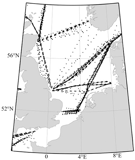
Figure 1. Location of the 5977 CPR sample points from 1998 to 2010, in the areas of the North Sea and English Channel (−4°W to 9°E and 48 to 60°N).

In this paper, a method was designed to label radiance anomalies (Ra(λ) thereafter) according to in-situ information provided by the CPR survey. The goal was to answer the following question: is there an empirical association between the presence of a diatom assemblage and specific radiance anomaly signals (as supported by the theoretical study of Alvain et al., 2012)? First, tools were developed and applied to extract suitable ecological information (i.e., diatom assemblages) from the CPR in-situ database (section 2.4.2). Second, the Ra(λ) was classified according to their form and amplitude (Ben Mustapha et al., 2014), and to their phenological characteristics (section 2.2). The objective of this second step was to fully characterize the Ra(λ) ranges in terms of shapes, amplitudes, and phenological behaviors in order to increase the chances of finding an association between specific in-situ diatom assemblages and a specific signal from remote-sensing. Finally, simultaneous in-situ and remote-sensing measurements were used to evaluate the relationships between the presence of diatom assemblages and the detection of specific radiance anomalies (sections 2.4.3 and 2.4.4).

2. Materials and Methods

Figure 2 displays the diagram of the process followed in this study. A list of definitions is available in the Supplementary Material (Supplementary Material Section 1, Definitions). These words are number indexed.

FIGURE 2

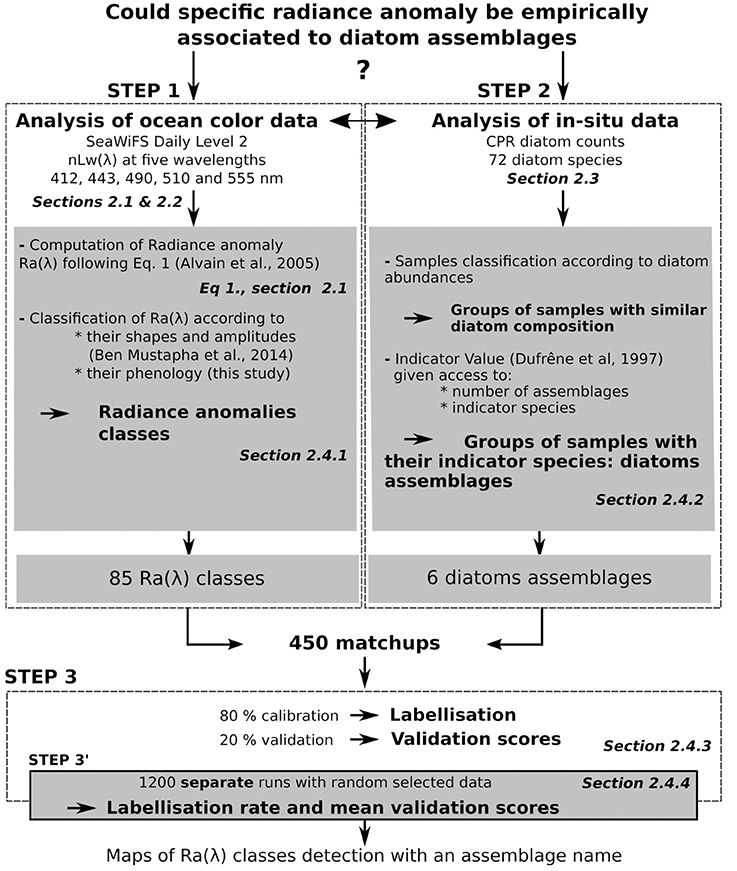
Figure 2. Diagram of the processing steps followed in this paper. For each step, the associated Section(s) is displayed in italic. The three main steps are framed with dotted lines. The first step involved the processing of remote-sensing data; the second step involved the processing of CPR data and the third step involved the test of association between the results of steps one and two.

The method used in this paper is based on the PHYSAT approach. Hence, a description of the general principle of the PHYSAT (Alvain et al., 2005, 2008) is given first, followed then by the actual process applied in this study.

2.1. General Principle of PHYSAT

The PHYSAT method is based on remote-sensed normalized water leaving radiances anomalies (Ra(λ))¹⁵. In fact, for a given chlorophyll-a concentration, it is possible to compute the mean value of radiances at each wavelength for the entire globe (2005 and 2014 versions) or specific regions (in present study, the North Sea was used). However, when considering one given pixel, associated with a chlorophyll-a concentration, the corresponding radiance values are slightly different from the global or regional mean. These differences can be characterized by the following Equation:

$\begin{array}{rc}\text{Ra}(\lambda )=\frac{\text{nLw}(\lambda )}{{\text{nLw}}_{\text{ref}}(\lambda ,\text{Chl-}a)}& (1)\end{array}$

Where Ra(λ) is the radiance anomaly at the sensor wavelengths, computed for each pixel; nLw(λ) is the observed normalized water-leaving radiance¹² at the same wavelength for a given pixel, and nLw_ref(λ, Chl-a) is the mean value of radiances at each wavelength and for a given chlorophyll-a.

Thus, when the value of Ra(λ) is greater than one, this indicates that the pixel has nLw(λ) values higher than the mean for the corresponding chlorophyll-a value. Whereas, when the value of Ra(λ) is less than one, this indicates that the pixel has nLw(λ) values lower than the mean. By considering the range of wavelength of a given remote sensor, it is possible to obtain Ra(λ) spectra with specific shape and amplitude, depending on the differences at each wavelength between the pixel values and the mean for the corresponding chlorophyll-a.

PHYSAT takes advantage of these small anomalies by empirically associating specific Ra(λ) shapes and amplitudes with a phytoplankton situation observed in-situ, through matchups¹⁰ exercise and in-situ investigations. Theoretical studies first brought an explanation for the specific shapes and amplitudes, showing that they are related to a combination of phytoplankton absorption, backscattering, and dissolved organic matter absorption (Alvain et al., 2012). All these parameters, when acting simultaneously on the light, produce specific anomalies around the mean radiance signal for a given chlorophyll-a concentration, associated with specific phytoplankton situation. To develop PHYSAT it is therefore necessary to have:

− Mean values of nLw(λ) for small ranges of chlorophyll-a. These mean values have to be computed for a given sensor in order to calculate a mean signal, including the characteristics of the sensor and processes

− Ra(λ) computed from the observed values and the above mean values following Equation 1; and then classified according to their shapes, amplitudes (Alvain et al., 2005; Ben Mustapha et al., 2014), and phenology (this study).

− A concurrent in-situ database with information on phytoplankton to empirically give a name to radiance anomalies

− Clear sky conditions (as define in Alvain et al., 2005) for matchups between the remote-sensing Ra and the in-situ data

Different approaches can be used to analyze Ra(λ) shapes and amplitudes. In the first version of PHYSAT (Alvain et al., 2005), large envelopes of minimum and maximum Ra(λ) values were used. This was in fact, the first time radiance anomalies had been analyzed. In Ben Mustapha et al. (2014), an improvement consisted of using a Self-Organizing Map (SOM hereafter) to classify the Ra(λ) more precisely and independently. Here, this last approach was used, in addition to some phenological tools (see section 2.4.1). Phenological tools allow, for instance, the separation of pixels with similar radiance anomalies (shape and amplitude), but with very different phenological characteristics (see the Figure S1 in the Supplementary Material for an illustration). These steps allow the grouping of the Ra(λ) into refined Ra(λ) classes¹⁶ with their specific shape, amplitude, and seasonal characteristics. Once this two-step classification is made, it is possible to empirically associate the Ra(λ) classes to a specific phytoplankton situation. In the 2005 (Alvain et al., 2005) and 2014 (Ben Mustapha et al., 2014) versions, biomarkers pigments were used for this step, allowing only the detection of dominance⁶ cases. Here, Ra(λ) spectra are associated with a more detailed in-situ database (CPR) in order to evaluate the potential of specific Ra(λ) for specific diatoms assemblages¹ in the surface waters. This last step aims to give a name to specific Ra(λ); names which could be completed each time new in-situ samples with Ra(λ) matchups are available.

2.2. Computation of PHYSAT Radiance Anomalies for This Study

In this study, the daily level 2 SeaWiFS remote-sensed normalized water leaving radiance (nLw, in the up-to-date version) between 1998 and 2004 in the English Channel and the North Sea (−4°W to 9°E and 48 to 60°N), with a resolution of 1 km², was used (NASA Goddard Space Flight Center, Ocean Ecology Laboratory, Ocean Biology Processing Group, 2014). The SeaWiFS data were selected instead of other ocean-color sensors due to the greater number of matchups with CPR data. Standard flags were applied to mask out pixels from clouds, ice, land, and sun-glint. In addition, pixels with aerosol optical thickness (at 865 nm) above 0.15 were excluded to ensure high atmospheric correction quality (Alvain et al., 2005). Furthermore, the classification proposed by Vantrepotte et al. (2012) was applied in this area to delineate waters with optical properties influenced by phytoplankton and associated CDOM³ (from phytoplankton degradation), and to flag waters influenced by other mineral particulate matters and potential remaining waters influenced by terrestrial origin CDOM. Radiance anomalies were subsequently computed by applying Equation 1 to selected data. The use of SeaWiFS data till 2004 ensured a homogeneous spatial coverage in the study area. Equation 1 was applied based on regional level 2 data in order to refine the study in the area of interest in this first attempt to highlight empirical links between phytoplankton assemblages and Ra(λ) classes. Subsequently, a specific mean signal for small ranges of chlorophyll-a (nLw_ref(λ, Chl-a) in Equation 1) was computed for the area under consideration.

2.3. In-Situ CPR Data

To evaluate the potential of PHYSAT in the detection of phytoplankton assemblages, it is necessary to make use of in-situ information about phytoplankton assemblages that may be potentially associated with a specific remote-sensing signal. An ideal in-situ database would be an inventory of all phytoplankton assemblages at a synoptic scale and with a high-repeat frequency over the course of one full calendar year (or longer). Unfortunately, such a database is currently not available. However, CPR data (SAHFOS, 2015) collected in the English Channel and North Sea, are particularly relevant in this first attempt to evaluate the potential of PHYSAT for the detection of diatom assemblages.

The Continuous Plankton Recorder survey is an upper layer plankton monitoring program that regularly collects samples in the North Atlantic and the North Sea, since 1946 (Reid et al., 2003). Studies have shown that this machine gives a satisfactory picture of the epipelagic zone (Lindley and Williams, 1980; Williams and Lindley, 1980). Inside the CPR machine, plankton are filtered by a moving band of silk—of mesh size 270 μm. These samples (which represent approximately 18 km of tow) are then analyzed later in the laboratory (Warner and Hays, 1994; Batten et al., 2003). Consequently, more than 400 species or taxa are identified and/or counted each month within the scale of the North Atlantic and its adjacent seas (Beaugrand, 2004). CPR phytoplankton abundance is a semi-quantitative estimate (see methods of abundance determination in Batten et al., 2003; Richardson et al., 2006, and Warner and Hays, 1994). However, the proportion of captured cells by the machine reflects major changes in abundance, distribution, and composition of phytoplankton (Robinson, 1970; Colebrook, 1982; Batten et al., 2003).

This in-situ dataset is unequaled in terms of size, spatio-temporal coverage, and representativeness of microphytoplankton abundance; it is classified into four groups: dinoflagellates, diatoms, silicoflagellates, and prymnesiophyceae. In particular, the CPR dataset (5,977 samples, Figure 1) recorded an abundance of 72 diatom species or taxa over the period 1998–2010, representing from 40 to 90% of the total microphytoplankton abundance in Summer (June-August) and Spring (March-June), respectively (Leterme et al., 2006). These diatoms are identified at a species or taxonomic level (one taxon could represent more than one species). Although diatoms are not alone in North Sea waters, and are associated with other types of phytoplankton (e.g., pico- and nano-phytoplankton), dealing with diatoms as an indicator of assemblages is the first step in describing phytoplankton communities. Thus, diatom assemblages are suitable to give a first answer to the following question: can specific radiance anomaly be empirically associated with the presence of a certain phytoplankton (here diatom) assemblages, as suggested by a previous theoretical study (Alvain et al., 2012)?

2.4. Processing Steps

2.4.1. Characterization of PHYSAT Radiance Anomalies: Step 1

The following processing steps correspond to Step 1 in Figure 2. The main objective was to characterize and classify the set of radiance anomalies. First, the regional radiance anomalies (computed by Equation 1) were classified according to their shape and amplitude by a Self-Organizing Map (SOM) algorithm (Kohonen, 2013) as previously defined in Ben Mustapha et al. (2014). Second, outgoing radiance anomaly classes were classified according to their phenological¹⁴ signature. This latter classification is supported by the hypotheses that two similar spectra (shape and amplitude)—(i) having the same phenology could be considered as identical; and (ii) having a different phenology could be associated with different in-situ situations.

So, to describe the characteristics of PHYSAT radiance anomalies, regional Ra(λ) spectra were classified by SOM into 100 sets of radiance anomalies following the approach of Ben Mustapha et al. (2014). However, this large number of Ra(λ) classes was potentially above the variability attainable by the phytoplankton. Consequently, the outputs of the SOM classification were adjusted to reflect the sought-after variability. To that purpose, a phenology-based classification was applied to group some of the 100 Ra(λ) classes, which presented almost identical seasonal characteristics based on occurrence frequencies (Figure 2, Step 1), by using conventional delineations of phenological characteristics (Platt et al., 2009). These metrics have been shown to be relevant at global and regional scales to characterize seasonal signals (e.g., Thackeray et al., 2008; Zhai et al., 2011; Racault et al., 2012). Timing of initiation¹⁴, maximum, termination¹⁴, and minimum, together with duration¹⁴ between (i) initiation and maximum, and (ii) maximum and termination, were used as multivariate characteristics for each Ra(λ) class; then used to regroup the Ra(λ) classes with the traditional UPGMA¹⁹ (Unweighted Pair Group Method with Arithmetic mean, Jain and Dubes, 1988) algorithm, based on an Euclidean distance. Analyses of classifications, based on different distances (Euclidean and Chord) and classification algorithms, did not alter the classifications (not shown here). Consequently, we selected the distance (here Euclidean) and the classification algorithm (here UPGMA) that yielded the best cophenetic correlation⁴ (Halkidi et al., 2001). The UPGMA classification was performed using a bootstrap re-sampling method to obtain robust groups of Ra(λ) classes, and verified by the Approximately Unbiased p-value (p < 0.05) (Shimodaira and Hasegawa, 2001; Shimodaira, 2002). The total number of Ra(λ) classes was downsized from 100 to 85, each representing a different radiance anomaly spectrum (shape and magnitude of the spectrum) and phenology (seasonal characteristics). At this stage, the 85 Ra(λ) classes are not associated with the presence of specific diatom assemblages in the surface open waters¹³. This last piece of information can be extracted from the CPR data analysis explained hereafter.

2.4.2. Characterization of Diatom Assemblages from in-Situ CPR Data: Step 2

The following processing steps correspond to Step 2 in Figure 2. The main objective was to analyze the large CPR database in order to obtain condensed ecological information suitable to be matched with Ra(λ) classes in Step 3. The CPR diatom counts recorded the occurrence of 72 diatom species and taxa. As mentioned above, diatoms were considered in this study as an indicator of the phytoplankton community composition; as such a species or taxa level description was not available from the other phytoplankton groups identified via CPR. The diatom species or taxa formed assemblages¹; some occurring in the same location at the same time according to their physical, chemical, and/or biological preferences (Sverdrup, 1953; Platt and Jassby, 1976). Before the calibration² step of PHYSAT, it was essential to assess recurrent in-situ diatom assemblages and their composition. For that purpose, the Indicator Value method (IndVal method, Dufrêne and Legendre, 1997) was chosen. This method has been successfully applied in various disciplines (e.g., Earth ecology, Chen et al., 2010; Ocean ecology, Darnis et al., 2008; medicine, Meadow et al., 2014; biochemistry, Schröder et al., 2015), and for various problems, e.g., climate change (Connor et al., 2013), and system pollution (Nahmani et al., 2006). It is a two-step approach: first, the samples are classified according to the composition and abundance of taxa; and second, an indicator value is computed according to the samples classification, allowing the indicator taxa or species⁸ to be highlighted. The IndVal (Indicator Value) method was selected to define the diatom assemblages because it deals with relative abundance and occurrence. It is based on a simple asymmetrical approach combining two criteria (the fidelity⁷ and the specificity¹⁸) to define a composite measure of the indicator value of each taxon with respect to a group of samples. Essentially, the measure of fidelity⁷ is at its maximum when a taxon occurs in only one group of samples; and specificity¹⁸, when a particular taxon is present in all samples of this group.

Assemblages characterization from the IndVal method first required the classification of CPR samples according to their diatom composition and abundances. The samples typology was obtained using an UPGMA classification algorithm¹⁹, based here on a dissimilarity distance computed on samples-standardized abundance of diatom taxa. The rare diatom taxa¹⁷ were removed from this classification step, leading to a database of 11 non-rare diatom taxa. Then, the next step was to determine the number of assemblages that had both a statistical and an ecological meaning as defined in Legendre and Legendre (2012), through the computation of the Indicator Value (Equation 2). The IndVal is computed for each possible cut-off level in typological samples (i.e., for each possible diatom assemblage). For example, the first cut-off level delineated two diatom assemblages, and the second one delineated three diatom assemblages—with their respective Indicator Value.

$\begin{array}{rc}\begin{array}{l}{\text{ A}}_{ij}={\text{Nindividuals}}_{ij}\text{/}{\text{Nindividuals}}_{i.}\\ {\text{ B}}_{ij}={\text{Nsamples}}_{ij}{\text{/Nsamples}}_{j.}\\ {\text{IndVal}}_{ij}={\text{A}}_{ij}\text{x}{\text{B}}_{ij}\end{array}& (2)\end{array}$

Where A_ij is a measure of specificity : Nindividuals_ij is the mean number of individuals of taxon i across group of samples j; and Nindividuals_i. is the sum of the mean number of individuals of taxon i over all groups of samples.

And B_ij is a measure of fidelity: Nsamples_ij is the number of samples in cluster j where taxon i occurs; and Nsamples_.j is the number of samples in cluster j

And IndVal_ij is the Indicator Value of the taxon i in the sample group j (Equations from Dufrêne and Legendre, 1997).

An ideal number of assemblages is reached when the Indicator Value does not increase significantly for a higher number of assemblages (see details in Dufrêne and Legendre, 1997; Aho et al., 2008). Please note that, the Indicator Value method was computed for the whole CPR diatom dataset (from 1998 to 2010) in order to reflect, as close as possible, the in-situ situations.

2.4.3. Calibration and Validation Procedure: Step 3

At this stage, in-situ diatom assemblages and classes of remote-sensing Ra(λ) (with different shape, magnitude, and phenology) were obtained. So, it was now possible to study potential matches between diatom assemblages and Ra(λ) classes. To achieve this, the in-situ CPR samples were matched to their associated satellite pixels (in a 3-by-3-pixel box corresponding to 9 km²) with a margin of ±3 h between the two measures (classical matchup¹⁰ procedures, referred in Bailey and Werdell, 2006, Figure 2, Step 3). The set of coincident measures (n_matchups = 450) was randomly divided in two subsets: a calibration subset (n_calibration = 360), and a validation subset (n_validation = 90); corresponding to 80 and 20% of the total number of matchups, respectively. The calibration step labeled⁹ empirically the radiance anomalies if, at least 50% of Ra(λ) class observations were assigned to the same in-situ assemblage in the calibration subset of matchups (this is the classical threshold used in PHYSAT, Alvain et al., 2005; Ben Mustapha et al., 2014).

Then, the radiance anomalies labeled with a diatom assemblage were subsequently validated with an independent subset (20% of CPR coincident measures, not used for calibration). The validation procedure considered only the labeled-Ra(λ). Here, the occurrence of labeled-Ra(λ) (one or more radiance anomaly classes) over the validation subset was checked. Ideally, in the validation subset, the labeled-Ra(λ) class has to be associated with the same diatom assemblage as the one which it was associated during the calibration (corresponding to a validation of 100%). Misclassification occurs when a Ra(λ) class is associated with a specific assemblage in the calibration step, but is found to correspond to another assemblage in the validation step. Furthermore, a misclassification occurs too when the specific labeled Ra(λ) class is not found in the validation subset.

2.4.4. Repetition of the Calibration Procedure: Step 3′

Because of the variability of the in-situ CPR data (in time and space), this calibration validation procedure was performed several times (number of separate procedures = 1,200) for different randomly-defined subsets of the calibration and validation to optimize the representativeness of the validation subset and strengthen the results (following a concept applied in ocean-color e.g., Craig et al., 2012; Bracher et al., 2015a; Brewin et al., 2015). This number of separate repetitions (n = 1,200) ensured that each randomly-selected matchup measurement was included at least once in the validation subset (Figure 2, Step 3). For each run of a calibration validation procedure, some Ra(λ) were labeled as a specific assemblage, followed by a validation percentage computation. This enabled the most robust Ra(λ) labels to be retained according to the rate of calibration, which meant that these labels had emerged regardless of the calibration and validation subsets.

3. Results

3.1. Indicator Taxa and Diatom Assemblages

The typology of CPR samples is displayed in Figure 3. According to this hierarchical clustering, the Indicator Value (IndVal, see section 2.4.2) was computed from level one (L1) to level six (L6)—see Table 1. For the first hierarchical subdivision in two groups (level 1, first Column of Table 1), only two diatom taxa were indicators (Chaetoceros spp2 and Thalassiosira spp.). From level 1 to 5 in Table 1, the number of indicator taxa increased, reaching six indicator taxa in level 5. The IndVal increased significantly among the first six hierarchical levels (or slightly decreased, insignificantly). There was an exception for the Thalassiosira spp., for which the IndVal values decreased significantly from level 1 to 5. This can be explained by the decrease in the specificity measure, whereas the fidelity measure was always at a maximum. The fifth level, differentiating six diatom assemblages, was the best one for which a compromise was found between the number of assemblages, the indicator taxon, and the IndVal values. Consequently, six diatom assemblages were retained, represented by an indicator diatom taxa and a set of secondary taxa. These assemblages are described in Table 2.

FIGURE 3

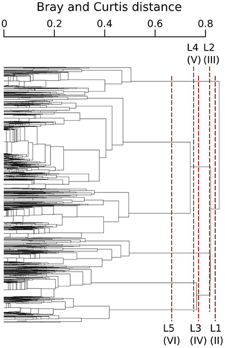
Figure 3. CPR samples typology obtained from the Bray-Curtis dissimilarity measure of the standardized abundance of diatoms and an UPGMA clustering algorithm. Each branch represents a CPR sample. L_x corresponds to x successive hierarchical clustering levels, giving a number of assemblages indicated by the roman number between parentheses.

TABLE 1

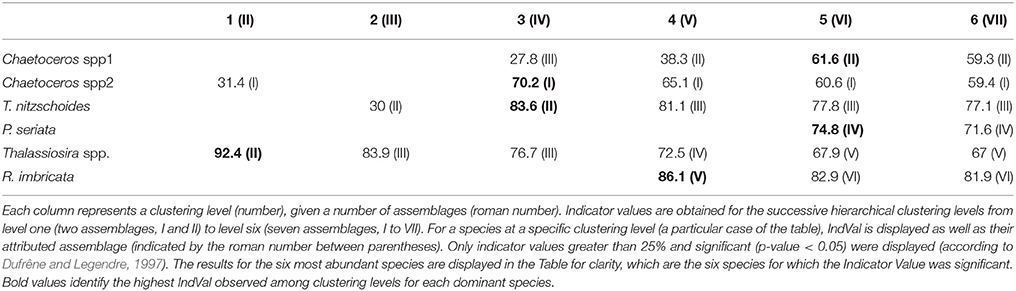
Table 1. This table represents a combination of the results from the classification of CPR samples and the computation of Indicator Values.

TABLE 2

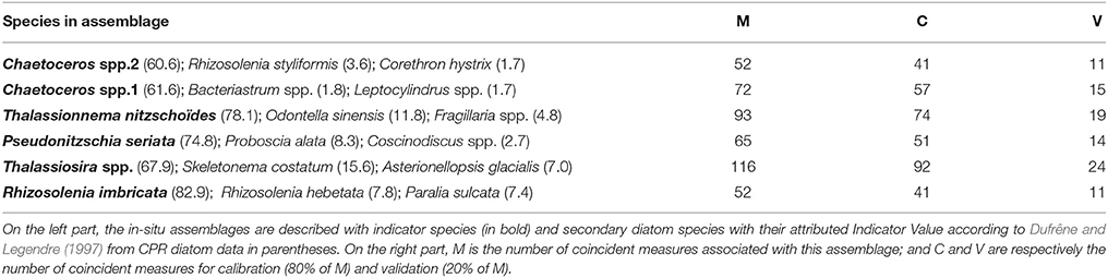
Table 2. This table represents information on in-situ data on the left part and on coincident measures on the right part.

3.2. Repetitive Calibration-Procedure

The number of matchups for each in-situ assemblage is presented in Column M (number of matchups) in Table 2. The calibration validation procedure was run 1,200 times to take into account the natural variability of the diatom assemblages. Figure 4 displays the number of times Ra(λ) was labeled for the 1,200 random calibration subsets. About 30% of Ra(λ) classes were never associated with an in-situ assemblage according to the criteria defined in the previous sections [for instance, Ra(λ) n°7 in Figure 4]. First, these Ra(λ) were either absent from the matchups or not present significantly to be labeled. Second, around 33% of Ra(λ) classes were associated with only one specific assemblage over the entire repetition procedure of calibration validation [for instance, Ra(λ) n°15 in Figure 4]. Finally, the remaining 37% of Ra(λ) classes were associated with multiple assemblages during the repetitive procedure [for instance, Ra(λ) n°25 in Figure 4]. These cases of multiple labeling were assumed to be possible considering that different phytoplanktonic communities can be associated with the presence of the diatom assemblage described here. For example, Ra(λ) n°57 in Figure 4, was labeled in less than 20% of calibration subsets; and labeled for half of the Thalassionema nitzschoides assemblage and half of the Thalassiosira spp. assemblage. For this Ra(λ) , the in-situ information available at this stage was not sufficient as this Ra(λ) was probably associated with a unidentified phytoplankton assemblage at this point. For a few number of Ra(λ) classes [example n°50 in Figure 4], the Ra(λ) were labeled in a large majority with the same assemblage. This depended upon the random separation of CPR samples in calibration and validation subsets; this result shows how necessary the repetition of the calibration was using a repetitive procedure. Only the assemblage labels which appeared in at least 70% of calibration repetitions (840 random calibration subsets) were retained. This threshold was chosen to ensure that the approach was robust enough for this first attempt in identifying specific radiance anomalies associated with the presence of a specific diatom assemblage. The threshold helped to retain only labeling that could be observed regardless of the calibration subset. Considering this threshold, the procedure led to the labeling of 11.7% of the 85 available Ra(λ) classes (total of Ra(λ) classes). Amongst the six in-situ diatom assemblages identified in the CPR dataset, three assemblages were robustly associated with ten Ra(λ) classes. In fact, during the 1200 repetitions of the calibration, assemblages characterized by Thalassionema nitzschoides, Thalassiosira sp., and Rhizosolenia imbricata, were associated with the one of the Ra(λ) classes more than 840 times (70% threshold). On the contrary, assemblages characterized by two taxa of Chaetoceros and by Pseudonitzschia seriata were not sufficiently associated with Ra(λ) classes in the multiple steps of calibration.

FIGURE 4

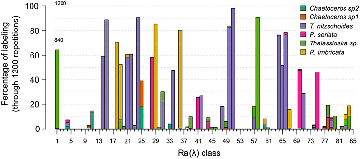
Figure 4. Percentage of Ra(λ) classes labeled with diatom assemblage(s) during the repetitive procedure of labeling including 1,200 random subsets of calibration. X axis represents the Ra(λ) classes identified by a number (1–85) and Y axis represents the rate of labeling of these Ra(λ) for the 1,200 random calibration-subsets. Each bar corresponds to the percentage of labeling of a specific Ra(λ) class (height) and associated with a specific in-situ assemblages indicated by the colors. See sections 2.4.3 and 2.4.4 for method of labeling and repetitive procedure. Blue dotted line represents the 70% threshold which define a robust labeling (section 3.2).

3.3. Radiance Anomaly Spectra Associated with Diatom Assemblages

Figure 5 displays the spectra of labeled-Ra(λ) classes associated with the three diatom assemblages. These Ra(λ) spectra are characterized by different amplitudes, shapes, and seasonalities. Note that these results were expected for intra-assemblage as well as inter-assemblage spectra variations in terms of shape and amplitude (see further information in section 4). Please also consider that, some Ra(λ) could appear very similar in terms of shape and amplitude, but their seasonal characteristics were different (an example is shown in Figure S1). The assemblage characterized by Thalassionema nitzschoides (Table 2) was associated with six different Ra(λ) classes (representing 7.1% of available Ra(λ) classes, Figure 5a for referent spectra) based on the available in-situ dataset. According to their shapes, these labeled Ra(λ) could be divided into two subgroups: high and low Ra(λ), at 412 and 443 nm, respectively. The assemblage characterized by Thalassiosira spp. was associated with one Ra(λ) class (1.2% of available Ra(λ), Figure 5b for referent spectrum). This reference spectrum had a straight shape. The Rhizosolenia imbricata assemblage was associated with three Ra(λ) classes (3.3% of available Ra(λ), Figure 5c for referent spectra). These spectra were different in shape and amplitude. At this stage, 10 Ra(λ) classes, with specific shapes, amplitudes, and seasonalities, were associated with three diatom assemblages, which were selected after the repetitive calibration validation procedure applied to the available CPR dataset.

FIGURE 5

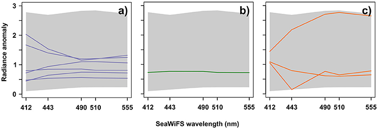
Figure 5. Labeled-radiance anomaly spectra (reference spectra of Ra(λ)) classes*) for (a) assemblage characterized by Thalassionema nitzschoides; (b) assemblage characterized by Thalassiosira spp.; and (c) assemblage characterized by Rhizosolenia imbricata. The gray background represents the entire diversity⁵ (minimum and maximum) of North Sea radiance anomalies spectra. X axis represents the five SeaWiFS wavelengths and the Y axis represents the radiance anomaly according to Equation (1). *The reference spectrum of a Ra(λ) class is computed from the Self-Organizing Map algorithm (SOM). It represents a compression of the information contained in all initial Ra(λ) spectra assigned in this specific Ra(λ) class by the SOM algorithm (Ben Mustapha et al., 2014).

3.4. Validation

Validation results are presented in Figure 6 and a summary of the validation scores is presented in Table 3. Figure 6 displays the mean validation scores (and standard deviation) for all Ra(λ) classes over the successive repetition of the calibration procedure. This highlights the variability of the validation scores, according to the variation of the calibration and validation subsets of matchups. The three assemblages for which a strong association could not be found with Ra(λ) had validation scores around 20% (see Total validation in Table 3). The validation for assemblages with a strong association with Ra(λ), as defined in section 2.4.4, is displayed in two ways. First, the total validation scores, which takes into account all labeled Ra(λ) (robustly-labeled or not), reached 61.8, 60.6, and 60.5%, respectively for Thalassionema nitzschoides assemblage, Thalassiosira spp. assemblage and Rhizosolenia imbricata assemblage (Table 3, column Total validation). These validation scores are increased by selecting the Ra(λ) according to the rate of labeling (70% threshold on repetitive calibration, see Figure 4 and section 2.4.4). Second, the validation scores reached 74.7, 95.2, and 63.8%, respectively, for Thalassionema nitzschoides assemblage, Thalassiosira spp. assemblage, and Rhizosolenia imbricata assemblage (Table 3, column Selected validation).

FIGURE 6

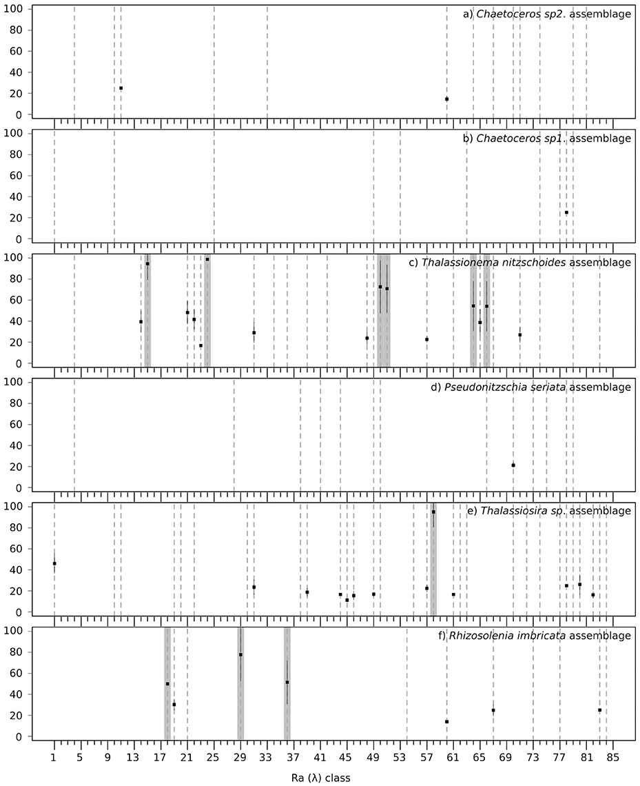
Figure 6. Mean validation scores (square points in percentage, Y axis) across the repetition of labeling procedure for the 85 Ra(λ) classes (X axis), with the standard deviation (black lines) for the six diatom assemblages: (a) Chaetoceros spp.2 assemblage, (b) Chaetoceros spp.1 assemblage, (c) Thalassionema nitzschoides assemblage, (d) Pseudonitzschia seriata assemblage, (e) Thalassiosira spp. assemblage, and (f) Rhizosolenia imbricata assemblage. A dotted line is drawn when the Ra(λ) class has been labeled as the assemblage at least one time. A gray background is drawn when the Ra(λ) class has been robustly labeled according to the rate of labeling (see Figure 4 and section 2.4.4). When the in-situ information is not sufficient to label and validate the association, only a dotted line is drawn (for example a), Ra(λ) °4).

TABLE 3

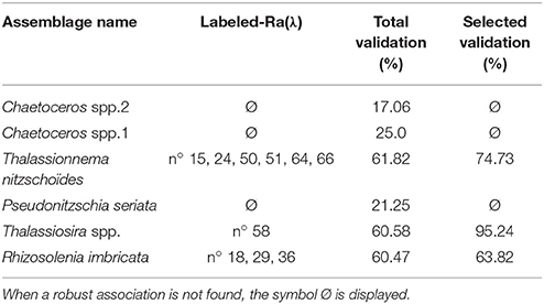
Table 3. This table represents the validation scores in two ways: (i) the total validation scores, which take into account all labeled-Ra(λ) in each 1,200 repetition of the calibration/validation procedure (average of all validation scores displayed in Figure 6) and (ii) the selected validation score according to the rate of labeling (see Figure 4 and section 2.4.4), which take into account only the robustly labeled-Ra(λ) (average of validation scores with a gray background in Figure 6).

3.5. Spatial and Seasonal Distribution of Ra(λ) Classes Associated with Diatom Assemblages

Specific labeled Ra(λ) were sought in the daily standard ocean-color maps with the aim of producing frequency detection maps. Monthly mean spatial frequencies of the labeled Ra(λ) are displayed in Figure 7. The frequency of occurrence of the labeled Ra(λ) for each pixel was averaged for each month over the period 1998–2004 (based on SeaWiFS data). It is worth to note that the frequency rarely rose above 0.5, except for a few pixels, suggesting that extension by additional Ra(λ) classes not labeled yet, opens the possibility for future investigations. The Ra(λ) identified as the Thalassionema nitzschoides assemblage (Figure 7A) showed their highest frequencies in spring (March and April) and fall (September and October). These classes were more frequently detected in the southern part of the North-Sea, the English Channel, and along the western coasts of the United Kingdom (UK). In the summer, the frequency of Ra(λ) classes associated with Thalassionema nitzschoides was low, and was located in the northern part of the North Sea and along the southern coasts of the UK. The frequency of the detection of the Ra(λ) class labeled as the Thalassiosira spp. assemblage showed a very low frequency (due to only one labeled Ra(λ), based on available in-situ dataset at this stage). This Ra(λ) class had its highest frequency in the middle of the year (June and July), and was mainly located in the middle of the North Sea (Figure 7B). The Ra(λ) classes identified as the Rhizosolenia imbricata assemblage exhibited a higher frequency in spring (March and April), which subsequently diminished during the following months, remaining low for the rest of the year. These labeled-Ra(λ) were located in the English Channel, and along the southern coast of the UK. In summer (June and July), a higher frequency pattern appeared near the Norwegian coast, which progressively disappeared during the following months (Figure 7C).

FIGURE 7

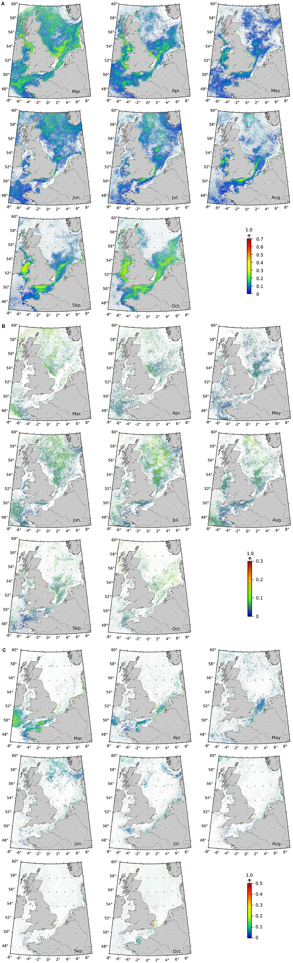
Figure 7. Climatology maps of labeled Ra(λ) classes detection frequencies (SeaWiFS level 2 data over 1998–2004) for Ra(λ) classes labeled as (A) Thalassionema nitzschoides assemblage ; (B) Thalassiosira spp. assemblage ; and (C) Rhizosolenia imbricata assemblage. Frequencies are computed by dividing the number of labeled Ra(λ) over the month (with a minimum of three occurrences) by the number of total Ra(λ) classes occurrence (labeled at this stage or not). If more than one Ra(λ) is labeled for a given assemblage, their frequencies are added. Please note that the color scales are different for the three distributions. White pixels means that less than 3 occurrences are recorded in the month. Due to high-solar zenith angle in the boreal Winter (November to February), signal could not be retrieved poleward 52°N and thus, only the results for the months of March to October are shown.

4. Discussion

4.1. Concerning the Choice of Indicator Value Method to Analyze CPR Diatom Counts

The indicator value method, combined with samples classification, allowed the identification of six diatom assemblages, each having their own seasonal cycle and geographical characteristics. These assemblages were stable over the period of 1998–2010 (in qualitative terms). For the five indicator taxa (Chaetoceros spp1, spp2, T. nitzschoides, P. seriata, and R. imbricata), the IndVal increased until the fifth clustering level of the CPR samples classification (reaching six assemblages), and then decreased, indicating that these taxa are stenotopic, i.e., they have a small niche¹¹ breadth (Dufrêne and Legendre, 1997). They also have a strong seasonality and a relatively limited spread, which has been commonly reported in the North Sea and English Channel (e.g., Reid et al., 1990; Rousseau et al., 2002; Hoppenrath, 2004; Bresnan et al., 2009; Hinder et al., 2012). On the contrary, Thalassiosira spp. IndVal decreased significantly among the successive hierarchical levels, indicating that this taxa is eurytopic, i.e., it has a large “niche breadth.” During the IndVal procedure, Thalassiosira spp. was the only one which was indicator at the taxa level (potentially more than one species), which probably explains the eurytopic behavior of this taxon. However, these results are supported by a number of studies, which have reported an increase in Thalassiosira spp. abundance and its spatial distribution (e.g., Bresnan et al., 2009; Hinder et al., 2012).

In this study, diatom assemblages were used as indicator of phytoplankton community composition. However, the three diatom assemblages highlighted here vary in terms of associated phytoplankton community, which has not been totally assessed at this point. From the CPR data, the dinoflagellates could be present with diatoms. Indeed, Thalassionema nitzschoides assemblage contributes an average of 93% of total microphytoplankton cells (7% of dinoflagellates cells), 83.2% for Thalassiosira spp. assemblage (16.8% of dinoflagellates cells), and 65.1% for Rhizosolenia imbricata assemblage (34.9% of dinoflagellates cells). So, the dinoflagellate community could partly explain the variability in terms of labeled-Ra(λ) characteristics (section 4.3), together with the other non-characterized community. Although dinoflagellates are present in the assemblages alongside diatoms, they are not classified as indicators according to Dufrêne and Legendre (1997).

Even if diatom assemblages are appropriate for this first evaluation of PHYSAT in the detection of assemblages, a more detailed in-situ database will be required in the future to take into account additional phytoplankton cases (more assemblages or taxonomic groups).

4.2. Spatio-Temporal Distribution of Labeled-Ra(λ)

Based on the CPR dataset available for this study, ten Ra(λ) classes (out of 85) were associated with three specific diatom assemblages in North Sea waters, with a high degree of confidence. The three other assemblages could not be robustly associated with Ra(λ) classes, according to our criteria (sections 2.4.3 and 2.4.4). For the ten Ra(λ) classes associated with diatom assemblages, monthly maps of Ra(λ) frequency show, for the first time, spatial and temporal variability in agreement with previously published literature in the North Sea (Reid et al., 1990; Beaugrand et al., 2001). In addition, the spatial distribution of all labeled-Ra(λ) classes followed known patterns relating to physical and hydrological conditions in the North Sea during the year that drive the phytoplankton distribution (Reid et al., 1990). In fact, four ecological regions have been commonly recorded based on phytoplankton, zooplankton, and fish studies in the North Sea (Daan et al., 1990; Reid et al., 1990; Fransz et al., 1991; Beaugrand et al., 2001). The Flamborough Front is a transitional region between the north of the front seasonally stratified and the south of the front (well-mixed area) (Otto et al., 1990; Ducrotoy et al., 2000). The fourth region is the Skagerrak, related to the Kattegat-Skagerrak flow (Otto et al., 1990). These regions have different conditions in nutrients, temperature, and available light, explaining that different phytoplankton assemblages could bloom according to their preferences (Margalef, 1978). The spatial distribution of labeled Ra(λ) frequencies delineated these four ecological regions.

Thalassionema nitzschoides and its associated taxa are dominant in winter, and bloom both in early spring and autumn in the North Sea (Figure 8A). The literature records show that their occurrence in some locations of the southern North Sea relates to specific environmental conditions (e.g., Edwards et al., 2001; Rousseau et al., 2002; Wiltshire et al., 2010). In fact, the assemblage characterized by Thalassionema nitzschoides is common in high-nutrient conditions in neritic waters (Van Iperen et al., 1993) as is the case in spring and autumn in the southern North Sea (Commission, 2010). The distribution of the labeled Ra(λ) was very similar to the literature on the occurrence and bloom of this assemblage.

FIGURE 8

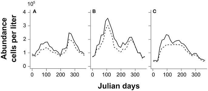
Figure 8. Mean seasonal abundance (10⁵ cells per liter) based on in-situ CPR counts between 1998 and 2010 for the labeled assemblages (solid lines) and their indicator species (dashed lines): (A) Thalassionema nitzschoides assemblage; (B) Thalassiosira spp. assemblage; and (C) Rhizosolenia imbricata assemblage.

The Rhizosolenia imbricata assemblage blooms in early spring with mixed waters, and maintains itself until summer (Figure 8C); taking place most of the time along the coastline (e.g., Hinder et al., 2012). The labeled Ra(λ) had a similar spatio-temporal distribution.

Concerning the assemblage composed by Thalassiosira spp., the literature has recorded a winter dominance, a spring blooming period, and a second autumn bloom since the 2000s (Hinder et al., 2012 and Figure 8B). Our results, based on the labeled Ra(λ) at this stage, show, in contrast, a higher frequency in summer in the core area of the North Sea. However, this difference could be due to the limited amount of information available to correctly detect this group. In fact, coincident measurements are sufficient for calibration in summer (71.5% of the Thalassiosira spp. assemblage matchups from May to August); while there were only a few matchups for the other months (28.5%, split in other months). Even if this Ra(λ) was correctly labeled, based on our first validation exercise ( 60% of correct identification), there are probably other winter, spring, and/or autumn radiance anomalies that may correspond to this assemblage. Thus, for the moment, the frequency of labeled anomaly signal remains low due to the small number of Ra(λ) classes with coincident in-situ measures.

4.3. Variability in Labeled-Ra(λ) Spectrum Characteristics in Terms of Shape, Amplitude and Seasonnality

The main characteristics of the Ra(λ) used in the past PHYSAT versions (Alvain et al., 2005, 2008; Ben Mustapha et al., 2014) are the shape and amplitude of the spectra (Alvain et al., 2012). In this study, the Ra(λ) have also been classified according to their phenology. This classification has two main advantages: (i) it avoids splitting the Ra(λ) classes (from the SOM algorithm), and therefore increases the chances of getting a larger number of coincident measurements; and (ii) it allows the distinction between two spectra that look similar in terms of shape and amplitude (as shown in Figure S1).

4.3.1. Intra- and Inter-assemblage Variation of Ra(λ) Characteristics

In some instances, one diatom assemblage could be associated with more than one Ra(λ) class (e.g., Thalassionema nitzschoides assemblage, which was associated with six Ra(λ) classes). These Ra(λ) spectra could be very different in terms of shape and amplitude. This is not surprising, as the shape and amplitude of Ra(λ) could vary with inherent optical properties due to phytoplankton characteristics and composition. In a theoretical study (Alvain et al., 2012) showed that radiance anomalies in PHYSAT results from a combination of (i) phytoplankton absorption, which affects both Ra(λ) shape and amplitude (especially at 443 nm); (ii) particulate backscattering, which strongly affects amplitude, but has a limited effect on the shape of Ra(λ); and (iii) CDOM (due to phytoplankton) absorption, which affects shape (mainly at 412 nm) and amplitude of the Ra(λ). This may explain why several Ra(λ) could be associated with different assemblages depending on: (a) the phytoplankton community composition associated with the diatom assemblage; (b) the growth stage, inducing different size, morphology, cells arrangement (including free cells, chains forming and aggregates), and pigment concentration; and (c) the CDOM concentration, sometimes reflecting the decline of a bloom.

The following hypotheses are proposed for the explanation of the inter-assemblage variations of radiance anomalies: (i) the morphology of cells: pennate (Thalassionema nitzschoides and Rhizosolenia imbricata), and oblate diatoms (Thalassiosira spp.); (ii) the arrangements of cells: the three characteristic diatoms could form chains (star, zigzag, and linear chains); (iii) cell sizes (from 2 to 230 μm, depending on growth stage); and (iv) associated phytoplankton communities. Intra-assemblage variations of radiance anomaly could be explained by: (i) the shift between free and chained cells; (ii) cell size variations; (iii) different species (in the case they are identified at taxa level) ; (iv) the shift in associated communities (e.g., from associated other diatoms to dinoflagellates); or (iv) the adaptation of pigments (quality and quantity), depending on available light and on the stage of the bloom.

All of the above hypotheses will need further investigations, considering in-situ optical parameters and a full characterization of phytoplankton communities, CDOM, and non-algal particles. Presently, it is impossible to isolate the contribution of inherent optical properties on the variation of radiance anomaly without in-situ or laboratory experiments (Alvain et al., 2012). However, the robustness of the labels and validation encourages us to complete more analyses following these approaches. Furthermore, the phenological tools applied to the Ra(λ) classification seems a promising tool for the calibration of PHYSAT.

4.3.2. “Multiple” Labeling Cases

The labeling-procedure shows that one Ra(λ) class could be successively linked to different assemblages depending on the calibration subset (cases of “multiple” labeling, see Figure 4, and section 3.2). Two different phytoplankton communities inducing the same radiance anomalies (depending on combinations of inherent optical properties) are rare cases according to Alvain et al. (2012), but are possible. In addition to an insufficient optical signal, this situation could also be explained by the presence of other phytoplankton communities associated with our diatom assemblages; not yet identified due to CPR data not available for other phytoplankton groups (pico-, and nano-phytoplankton). However, the validation scores observed in this study are encouraging, and also highlight the fact that a large number of Ra(λ) classes remain unattributed to any specific assemblage, indicating that our approach could be further completed. Future in-situ measurements coupling phytoplankton analyses and optical properties are strongly needed to ameliorate our procedure and identify whether specific Ra(λ) classes associated with many phytoplankton cases exist. The addition of phenology to classify the Ra(λ) reduces misclassification. Indeed, different optical properties leading to a similar spectra and phenology are considered as rare, based on current knowledge.

4.4. Remaining Ra(λ) Database, Limitations, and Perspectives

For this first attempt to evaluate PHYSAT in non-dominance cases detection, very stringent steps were chosen, with a high degree selection (such as the 70% threshold on the rate of labeling). Potential future extension of this method, with additional in-situ data (hopefully not just limited to diatoms) will have to find a balance between strict thresholds, dataset availability, and score of validation. If the proposed method allows the identification of 11.7% of the available Ra(λ) classes at this stage, the remaining anomaly classes are available for future investigation and empirical labeling. Figure 9 illustrates the potential of PHYSAT development by showing spatial distribution of the most frequently detected Ra(λ) classes in the North Sea. The Ra(λ) classes in Figure 9 show a clear seasonal succession, as the most frequent Ra(λ) classes are not the same between months. Furthermore, their spatial distributions delineate specific patterns in agreement with the environmental conditions described above (ecological regions in the North Sea). The 88.3% remaining unlabeled Ra(λ) classes could represent: (i) one of the diatom assemblages described here, at a different step of development, or associated with different non-diatom phytoplankton species (with no-matchup at the moment); or (ii) other unidentified assemblages of phytoplankton. In fact, the North Sea is a highly variable environment for phytoplankton, mostly dominated by diatoms (winter, spring, and autumn) and dinoflagellates (summer), but also by Prymnesiophyceae (such Phaeocystis sp.), Chlorophyceae, Cyanobacteria, and sometimes Coccolithophorids (Gieskes and Kraay, 1983; Reid et al., 1990; Hoppenrath, 2004; Hoppenrath et al., 2007; Sapp et al., 2007; Masquelier et al., 2011; Bonato et al., 2015).

FIGURE 9

Figure 9. Maps of most frequently detected radiance anomalies classes in the North Sea in March (A), June (B), and October (C). The color bar displays the 85 different Ra(λ) classes (0–85). The color corresponds to the Ra(λ) class (identify by a number) with the highest frequency in a specific pixel and month.

If this study shows the potential of detection of phytoplankton situations beyond the dominance, there are still developments to be carried out with other in-situ information to characterize phytoplankton community. Although non-quantitative, these observations would be useful to estimate the contribution of assemblages to the chlorophyll-a estimation (Alvain et al., 2006, 2008) and then completing approaches such as OC-PFT (Hirata et al., 2011), PhytoDAS (Bracher et al., 2009). In this way, we support that development of in-situ measurements will allow us to identify more phytoplankton assemblages and better understand the limitation of this empirical approach. Some preliminary investigations, based on in-situ data, have shown that the Ra(λ) classes associated with diatoms assemblages previously characterized would not be associated with other groups (especially microphytoplankton as dinoflagellates) (not shown here). This observation is valid only for the Ra(λ) classes considered as robustly labeled, which would confirm that cases of multiple labeling (in the repetition of the calibration procedure) are due to other phytoplankton assemblages. These investigations will be considered in future developments.

Further studies will be required in the future to assess three main concerns about PHYSAT. First, a full characterization of the phytoplankton community and their optical properties during a bloom could permit us to analyze the variations of the radiance anomaly in terms of shape and amplitude, and to understand the optical justification of the empirical linkage (Alvain et al., 2012). Then, the CPR measurements are based on moving samples representing 18 km of tow, which may lead to a biased location of the sample and thereby on the matchups measurements. This has been considered in this study by observing the homogeneity of the remote-sensing observations within 3 days. This point needs to be considered for future studies, especially for a study of the Ra(λ) characteristics. Second, the requirements for regional algorithms have to be estimated by studying other regions. Previous studies have already demonstrated that regional ocean-color algorithms are sometimes necessary (for example, Volpe et al., 2007 for the Mediterranean Sea). The regional approach of PHYSAT developed for this first evaluation is not comparable to the global approach due to the use of specific reference tables in these two cases. Third, PHYSAT requires a specific reference table (see Equation 1) for each ocean-color sensor. For now, it is difficult to evaluate the uncertainties during the transition of the PHYSAT labels from one sensor to another one. Thus, impacts of multi-sensors inter-calibration will have to be carefully addressed before PHYSAT application to standardized remote-sensing database. That is one reason why we greatly support the development of in-situ measurements to carry out a new calibration and/or to validate the transposition of labels between ocean-color sensors.

5. Conclusion

PHYSAT (Alvain et al., 2005, 2008) is an ocean-color algorithm that has allowed us to identify five phytoplankton groups based on ocean-color radiance anomalies analysis in terms of shape and amplitude. However, this empirical algorithm was limited to dominant cases due to the use of biomarker pigment ratios in the empirical calibration step. In this study, we took advantage of both the addition of phenological tools to analyze the radiance anomalies and the diatom species abundance data to evaluate the PHYSAT potential in terms of phytoplankton assemblages detection. The use of abundance data in the PHYSAT calibration step presents a promising avenue for future investigations and development of PFT algorithms. Although this study is based on a limited number of assemblages at this stage, it demonstrates the potential of development of the PHYSAT method beyond the dominance case, toward the detection of phytoplankton assemblages. Three diatom assemblages were successfully associated with specific ocean-color radiance anomalies with a robust validation. For now, there are no scientific reasons to prevent the use of PHYSAT radiance anomalies in other non-coastal waters and to associate remaining radiance anomalies with other assemblages. This first attempt to compute maps of signals associated with specific diatom assemblages highlights distinct spatial and temporal patterns in agreement with previous knowledge. Thyssen et al. (2015) showed that it is possible to describe the community structure at the basin-scale by comparing high resolution techniques (cytometry) and remote-sensing radiance anomalies. These recent results support both the development of PHYSAT beyond dominance-case detection, as well as the strong need of additional in-situ information about phytoplankton assemblages. This last objective could not only be performed based on CPR observations, but also on automated in-situ analysis such as cytometry (Thyssen et al., 2015) or DNA sequencing approaches (Ottesen et al., 2011). Indeed, PHYSAT calibration is not limited to a specific type of data and only requires homogeneous datasets. Approaches based on ocean-color signal analysis, empirically coupled with exhaustive in-situ measurements (phytoplankton and optical properties) will help us to further understand which and how environmental conditions drive the phytoplankton composition and its succession, together with potential applications in the investigation of long-term changes.

Author Contributions

All authors contributed to the conception of the work, data analysis and interpretations. A-HR-L and SA drafted the article and all authors contributed to the critical revision of the article and made improvements. All authors approved the final version.

Funding

This work was founded by the CNES/TOSCA program, CNRS and Hauts-de-France region. MR was partially supported by the European Space Agency Living Planet Fellowship program grant number 4000112798/15/I/SBo.

Conflict of Interest Statement

The authors declare that the research was conducted in the absence of any commercial or financial relationships that could be construed as a potential conflict of interest.

Acknowledgments

The authors would like to thank NASA/GSFC/DAAC for providing access to daily SeaWiFS products and the Sir Alistair Hardy Foundation for Ocean Science (SAHFOS) for providing in-situ observations from CPR. www.englisheditor.webs.com is thanked for its English proofing. David Antoine, Annick Bricaud, Lucile Duforêt-Gaurier, Hubert Loisel, Bertrand Lubac, and Julia Uitz are thanked for their valuable comments on an earlier draft of this paper. Experiments presented in this paper were carried out using the CALCULCO computing platform, supported by SCoSI/ULCO (Service COmmun du Système d'Information de l'Université du Littoral Côte d'Opale).

Supplementary Material

The Supplementary Material for this article can be found online at: https://www.frontiersin.org/articles/10.3389/fmars.2017.00408/full#supplementary-material

References

Aho, K., Roberts, D. W., and Weaver, T. (2008). Using geometric and non-geometric internal evaluators to compare eight vegetation classification methods. J. Veget. Sci. 19, 549–562. doi: 10.3170/2008-8-18406

CrossRef Full Text | Google Scholar

Aiken, J., Fishwick, J. R., Lavender, S., Barlow, R., Moore, G. F., Sessions, H., et al. (2007). Validation of MERIS reflectance and chlorophyll during the BENCAL cruise October 2002: preliminary validation of new demonstration products for phytoplankton functional types and photosynthetic parameters. Int. J. Remote Sens. 28, 497–516. doi: 10.1080/01431160600821036

CrossRef Full Text | Google Scholar

Alvain, S., Loisel, H., and Dessailly, D. (2012). Theoretical analysis of ocean color radiances anomalies and implications for phytoplankton groups detection in case 1 waters. Opt. Exp. 20, 1070–1083. doi: 10.1364/OE.20.001070

PubMed Abstract | CrossRef Full Text | Google Scholar

Alvain, S., Moulin, C., Dandonneau, Y., and Bréon, F. (2005). Remote sensing of phytoplankton groups in case 1 waters from global seawifs imagery. Deep Sea Res. I 52, 1989–2004. doi: 10.1016/j.dsr.2005.06.015

CrossRef Full Text | Google Scholar

Alvain, S., Moulin, C., Dandonneau, Y., and Loisel, H. (2008). Seasonal distribution and successuib of dominant phytoplankton groups in the global ocean: a satellite view. Glob. Biogeochem. Cycles 22, 1–15. doi: 10.1029/2007GB003154

CrossRef Full Text | Google Scholar

Alvain, S., Moulin, C., Dandonneau, Y., Loisel, H., and Bréon, F.-M. (2006). A species-dependant bio-optical model of case i waters for global ocean color processing. Deep Sea Res. I 53, 917–925. doi: 10.1016/j.dsr.2006.01.011

CrossRef Full Text | Google Scholar

Bailey, S. W., and Werdell, P. J. (2006). A multi-sensor approach for the on-orbit validation of ocean color satellite data products. Remote Sens. Environ. 102, 12–23. doi: 10.1016/j.rse.2006.01.015

CrossRef Full Text | Google Scholar

Batten, S., Clark, R., Flinkman, J., Hays, G., John, E., John, A., et al. (2003). Cpr sampling: the technical background, materials and methods, consistency and comparability. Prog. Oceanogr. 58, 193–215. doi: 10.1016/j.pocean.2003.08.004

CrossRef Full Text | Google Scholar

Beaugrand, G. (2004). Continuous plankton records: plankton atlas of the north atlantic ocean (1958-1999). I. Introduction and methodology. Mar. Ecol. Prog. Ser. 268, 3–10. doi: 10.3354/mepscpr003

CrossRef Full Text | Google Scholar

Beaugrand, G. (2015). Marine Biodiversity, Climatic Variability and Global Change. Oxon; New York, NY: Routledge.

Google Scholar

Beaugrand, G., Ibañez, F., and Lindley, J. A. (2001). Geographical distribution and seasonal and diel changes of the diversity of calanoid copepods in the north atlantic and north sea. Mar. Ecol. Prog. Ser. 219, 189–203. doi: 10.3354/meps219189

CrossRef Full Text | Google Scholar

Ben Mustapha, Z., Alvain, S., Jamet, C., Loisel, H., and Dessailly, D. (2014). Automatic classification of water-leaving radiance anomalies from global seawifs imagery: application to the detection of phytoplankton groups in open ocean waters. Remote Sens. Environ. 146, 97–112. doi: 10.1016/j.rse.2013.08.046

CrossRef Full Text | Google Scholar

Bonato, S., Christaki, U., Lefebvre, A., Lizon, F., Thyssen, M., and Artigas, L. F. (2015). High spatial variability of phytoplankton assessed by flow cytometry, in a dynamic productive coastal area, in spring: the eastern english channel. Estuar. Coast. Shelf Sci. 154, 214–223. doi: 10.1016/j.ecss.2014.12.037

CrossRef Full Text | Google Scholar

Boss, E., Slade, W., and Hill, P. (2009). Effect of particulate aggregation in aquatic environments on the beam attenuation and its utility as a proxy for particulate mass. Opt. Exp. 17, 9408–9420. doi: 10.1364/OE.17.009408

PubMed Abstract | CrossRef Full Text | Google Scholar

Bracher, A., Hardman-Mountford, N., Hirata, T., Bernard, S., Boss, E., Brewin, R., et al. (2015a). “Report on ioccg workshop: phytoplankton composition from space: towards a validation strategy for satellite algorithms,” in The International Ocean-Colour Coordinating Group (IOCCG) 25-26 October 2014)(NASA/TM-2015-217528 (Portland, ME).

Google Scholar

Bracher, A., Taylor, M., Taylor, B., Dinter, T., Roettgers, R., and Steinmetz, F. (2015b). Using empirical orthogonal functions derived from remote sensing reflectance for the prediction of phytoplankton pigments concentrations. Ocean Sci. 11, 139–158. doi: 10.5194/os-11-139-2015

CrossRef Full Text | Google Scholar

Bracher, A., Vountas, M., Dinter, T., Burrows, J., Röttgers, R., and Peeken, I. (2009). Quantitative observation of cyanobacteria and diatoms from space using PhytoDOAS on SCIAMACHY data. Biogeosciences 6, 751–764. doi: 10.5194/bg-6-751-2009

CrossRef Full Text | Google Scholar

Bresnan, E., Hay, S., Hughes, S., Fraser, S., Rasmussen, J., Webster, L., et al. (2009). Seasonal and interannual variation in the phytoplankton community in the north east of scotland. J. Sea Res. 61, 17–25. doi: 10.1016/j.seares.2008.05.007

CrossRef Full Text | Google Scholar

Brewin, R. J., Hardman-Mountford, N. J., Lavender, S. J., Raitsos, D. E., Hirata, T., Uitz, J., et al. (2011). An intercomparison of bio-optical techniques for detecting dominant phytoplankton size class from satellite remote sensing. Remote Sens. Environ. 115, 325–339. doi: 10.1016/j.rse.2010.09.004

CrossRef Full Text | Google Scholar

Brewin, R. J., Sathyendranath, S., Jackson, T., Barlow, R., Brotas, V., Airs, R., et al. (2015). Influence of light in the mixed-layer on the parameters of a three-component model of phytoplankton size class. Remote Sens. Environ. 168, 437–450. doi: 10.1016/j.rse.2015.07.004

CrossRef Full Text | Google Scholar

Bricaud, A., Ciotti, A., and Gentili, B. (2012). Spatial-temporal variations in phytoplankton size and colored detrital matter absorption at global and regional scales, as derived from twelve years of seawifs data (1998–2009). Glob. Biogeochem. Cycles 26:GB1010. doi: 10.1029/2010GB003952

CrossRef Full Text | Google Scholar

Bricaud, A., and Morel, A. (1986). Light attenuation and scattering by phytoplanktonic cells: a theoretical modeling. Appl. Opt. 25, 571–580. doi: 10.1364/AO.25.000571

PubMed Abstract | CrossRef Full Text | Google Scholar

Chen, L., Mi, X., Comita, L. S., Zhang, L., Ren, H., and Ma, K. (2010). Community-level consequences of density dependence and habitat association in a subtropical broad-leaved forest. Ecol. Lett. 13, 695–704. doi: 10.1111/j.1461-0248.2010.01468.x

PubMed Abstract | CrossRef Full Text | Google Scholar

Clavano, W., Boss, E., and Karp-Boss, L. (2007). Inherent optical properties of non-spherical marine-like particles from theory to observation. Oceanogr. Mar. Biol. 45, 1–38. doi: 10.1201/9781420050943.ch1

CrossRef Full Text | Google Scholar

Colebrook, J. (1982). Continuous plankton records-phytoplankton, zooplankton and environment, northeast atlantic and north-sea, 1958-1980. Oceanol. Acta 5, 473–480.

Google Scholar

Commission, O. (2010). Bilan de Santé 2010. London: Commision OSPAR.

Connor, S. E., Ross, S. A., Sobotkova, A., Herries, A. I., Mooney, S. D., Longford, C., et al. (2013). Environmental conditions in the se balkans since the last glacial maximum and their influence on the spread of agriculture into europe. Q. Sci. Rev. 68, 200–215. doi: 10.1016/j.quascirev.2013.02.011

CrossRef Full Text | Google Scholar

Craig, S. E., Jones, C. T., Li, W. K., Lazin, G., Horne, E., Caverhill, C., et al. (2012). Deriving optical metrics of coastal phytoplankton biomass from ocean colour. Remote Sens. Environ. 119, 72–83. doi: 10.1016/j.rse.2011.12.007

CrossRef Full Text | Google Scholar

Daan, N., Bromley, P., Hislop, J., and Nielsen, N. (1990). Ecology of north sea fish. Netherlands J. Sea Res. 26, 343–386. doi: 10.1016/0077-7579(90)90096-Y

CrossRef Full Text | Google Scholar

Darnis, G., Barber, D. G., and Fortier, L. (2008). Sea ice and the onshore–offshore gradient in pre-winter zooplankton assemblages in southeastern beaufort sea. J. Mar. Syst. 74, 994–1011. doi: 10.1016/j.jmarsys.2007.09.003

CrossRef Full Text | Google Scholar

De Monte, S., Soccodato, A., Alvain, S., and d'Ovidio, F. (2013). Can we detect oceanic biodiversity hotspots from space? ISME J. 7, 2054–2056. doi: 10.1038/ismej.2013.72

PubMed Abstract | CrossRef Full Text | Google Scholar

Devred, E., Sathyendranath, S., Stuart, V., and Platt, T. (2011). A three component classification of phytoplankton absorption spectra: application to ocean-color data. Remote Sens. Environ. 115, 2255–2266. doi: 10.1016/j.rse.2011.04.025

CrossRef Full Text | Google Scholar

D'Ovidio, F., De Monte, S., Alvain, S., Dandonneau, Y., and Lévy, M. (2010). Fluid dynamical niches of phytoplankton types. Proc. Natl. Acad. Sci. U.S.A. 107, 18366–18370. doi: 10.1073/pnas.1004620107

PubMed Abstract | CrossRef Full Text | Google Scholar

Dubelaar, G. B., Visser, J. W., and Donze, M. (1987). Anomalous behaviour of forward and perpendicular light scattering of a cyanobacterium owing to intracellular gas vacuoles. Cytometry 8, 405–412. doi: 10.1002/cyto.990080410

PubMed Abstract | CrossRef Full Text | Google Scholar

Ducrotoy, J.-P., Elliott, M., and de Jonge, V. N. (2000). The north sea. Mar. Pollut. Bull. 41, 5–23. doi: 10.1016/S0025-326X(00)00099-0

CrossRef Full Text | Google Scholar

Duforêt-Gaurier, L., Loisel, H., Dessailly, D., Nordkvist, K., and Alvain, S. (2010). Estimates of particulate organic carbon over the euphotic depth from in situ measurements. Application to satellite data over the global ocean. Deep Sea Res. I Oceanogr. Res. Papers 57, 351–367. doi: 10.1016/j.dsr.2009.12.007

CrossRef Full Text | Google Scholar

Dufrêne, M., and Legendre, P. (1997). Species assemblages and indicator species: the need for a flexible asymmetrical approach. Ecol. Monogr. 67, 345–366. doi: 10.2307/2963459

CrossRef Full Text | Google Scholar

Edwards, M., Reid, P., and Planque, B. (2001). Long-term and regional variability of phytoplankton biomass in the northeast atlantic (1960–1995). ICES J. Mar. Sci. 58, 39–49. doi: 10.1006/jmsc.2000.0987

CrossRef Full Text | Google Scholar

Falkowski, P. G. (1994). The role of phytoplankton photosynthesis in global biogeochemical cycles. Photosynth. Res. 39, 235–258. doi: 10.1007/BF00014586

PubMed Abstract | CrossRef Full Text | Google Scholar

Fransz, H., Colebrook, J., Gamble, J., and Krause, M. (1991). The zooplankton of the north sea. Netherlands J. Sea Res. 28, 1–52. doi: 10.1016/0077-7579(91)90003-J

CrossRef Full Text | Google Scholar

Gieskes, W., and Kraay, G. (1983). Dominance of cryptophyceae during the phytoplankton spring bloom in the central north sea detected by hplc analysis of pigments. Mar. Biol. 75, 179–185. doi: 10.1007/BF00406000

CrossRef Full Text | Google Scholar

Halkidi, M., Batistakis, Y., and Vazirgiannis, M. (2001). On clustering validation techniques. J. Intel. Inform. Syst. 17, 107–145. doi: 10.1023/A:1012801612483

CrossRef Full Text | Google Scholar

Hinder, S. L., Hays, G. C., Edwards, M., Roberts, E. C., Walne, A. W., and Gravenor, M. B. (2012). Changes in marine dinoflagellate and diatom abundance under climate change. Nat. Clim. Change 2, 271–275. doi: 10.1038/nclimate1388

CrossRef Full Text | Google Scholar

Hirata, T., Hardman-Mountford, N. J., Brewin, R. J. W., Aiken, J., Barlow, R., Suzuki, K., et al. (2011). Synoptic relationships between surface Chlorophyll-a and diagnostic pigments specific to phytoplankton functional types. Biogeosciences 8, 311–327. doi: 10.5194/bg-8-311-2011

CrossRef Full Text | Google Scholar

Hood, R. R., Laws, E. A., Armstrong, R. A., Bates, N. R., Brown, C. W., Carlson, C. A., et al. (2006). Pelagic functional group modeling: progress, challenges and prospects. Deep Sea Res. II Top. Stud. Oceanogr. 53, 459–512. doi: 10.1016/j.dsr2.2006.01.025

CrossRef Full Text | Google Scholar

Hoppenrath, M. (2004). A revised checklist of planktonic diatoms and dinoflagellates from helgoland (north sea, german bight). Helgoland Mar. Res. 58, 243–251. doi: 10.1007/s10152-004-0190-6

CrossRef Full Text | Google Scholar

Hoppenrath, M., Beszteri, B., Drebes, G., Halliger, H., Van Beusekom, J. E., Janisch, S., et al. (2007). Thalassiosira species (bacillariophyceae, thalassiosirales) in the north sea at helgoland (german bight) and sylt (north frisian wadden sea)–a first approach to assessing diversity. Eur. J. Phycol. 42, 271–288. doi: 10.1080/09670260701352288

CrossRef Full Text | Google Scholar

Jain, A. K., and Dubes, R. C. (1988). Algorithms for Clustering Data. Upper Saddle River, NJ: Prentice-Hall, Inc.

Google Scholar

Kirk, J. T. (1994). Light and Photosynthesis in Aquatic Ecosystems. Cambridge: Cambridge University Press.

Google Scholar

Kohonen, T. (2013). Essentials of the self-organizing map. Neural Netw. 37, 52–65. doi: 10.1016/j.neunet.2012.09.018

PubMed Abstract | CrossRef Full Text | Google Scholar

Kostadinov, T., Siegel, D., and Maritorena, S. (2009). Retrieval of the particle size distribution from satellite ocean color observations. J. Geophys. Res. Oceans 114, 1–22. doi: 10.1029/2009JC005303

CrossRef Full Text | Google Scholar

Kostadinov, T., Siegel, D., and Maritorena, S. (2010). Global variability of phytoplankton functional types from space: assessment via the particle size distribution. Biogeosciences 7, 3239–3257. doi: 10.5194/bg-7-3239-2010

CrossRef Full Text | Google Scholar

Kump, L. R., Kasting, J. F., and Crane, R. G. (2010). The Earth System. San Francisco, CA: Prentice Hall.

PubMed Abstract | Google Scholar

Le Quéré, C., Harrison, S. P., Colin Prentice, I., Buitenhuis, E. T., Aumont, O., Bopp, L., et al. (2005). Ecosystem dynamics based on plankton functional types for global ocean biogeochemistry models. Glob. Change Biol. 11, 2016–2040. doi: 10.1111/j.1365-2486.2005.1004.x

CrossRef Full Text | Google Scholar

Legendre, P., and Legendre, L. F. (2012). Numerical Ecology, Vol. 24. Oxford: Elsevier.

Google Scholar

Leterme, S. C., Seuront, L., and Edwards, M. (2006). Differential contribution of diatoms and dinoflagellates to phytoplankton biomass in the ne atlantic ocean and the north sea. Mar. Ecol. Prog. Ser. 312, 57–65. doi: 10.3354/meps312057

CrossRef Full Text | Google Scholar

Li, Z., Li, L., Song, K., and Cassar, N. (2013). Estimation of phytoplankton size fractions based on spectral features of remote sensing ocean color data. J. Geophys. Res. Oceans 118, 1445–1458. doi: 10.1002/jgrc.20137

CrossRef Full Text | Google Scholar

Lindley, J., and Williams, R. (1980). Plankton of the fladen ground during flex 76 II. Population dynamics and production of Thysanoessa inermis (crustacea: Euphausiacea). Mar. Biol. 57, 79–86. doi: 10.1007/BF00387373

CrossRef Full Text | Google Scholar

Margalef, R. (1978). Life-forms of phytoplankton as survival alternatives in an unstable environment. Oceanol. Acta 1, 493–509.

Google Scholar

Masquelier, S., Foulon, E., Jouenne, F., Ferréol, M., Brussaard, C. P., and Vaulot, D. (2011). Distribution of eukaryotic plankton in the english channel and the north sea in summer. J. Sea Res. 66, 112–122. doi: 10.1016/j.seares.2011.05.004

CrossRef Full Text | Google Scholar

Meadow, J. F., Altrichter, A. E., Kembel, S. W., Moriyama, M., O'Connor, T. K., Womack, A. M., et al. (2014). Bacterial communities on classroom surfaces vary with human contact. Microbiome 2, 1–7. doi: 10.1186/2049-2618-2-7

PubMed Abstract | CrossRef Full Text

Morel, A., and Bricaud, A. (1981). Theoretical results concerning light absorption in a discrete medium, and application to specific absorption of phytoplankton. Deep Sea Res. A Oceanogr. Res. Papers 28, 1375–1393. doi: 10.1016/0198-0149(81)90039-X

CrossRef Full Text | Google Scholar

Mouw, C. B., Hardman-Mountford, N. J., Alvain, S., Bracher, A., Brewin, R. J., Bricaud, A., et al. (2017). A consumer's guide to satellite remote sensing of multiple phytoplankton groups in the global ocean. Front. Mar. Sci. 4:41. doi: 10.3389/fmars.2017.00041

CrossRef Full Text | Google Scholar

Mouw, C. B., and Yoder, J. A. (2010). Optical determination of phytoplankton size composition from global seawifs imagery. J. Geophys. Res. Oceans 115:C12018. doi: 10.1029/2010JC006337

CrossRef Full Text | Google Scholar

Nahmani, J., Lavelle, P., and Rossi, J.-P. (2006). Does changing the taxonomical resolution alter the value of soil macroinvertebrates as bioindicators of metal pollution? Soil Biol. Biochem. 38, 385–396. doi: 10.1016/j.soilbio.2005.04.037

CrossRef Full Text | Google Scholar

Nair, A., Sathyendranath, S., Platt, T., Morales, J., Stuart, V., Forget, M.-H., et al. (2008). Remote sensing of phytoplankton functional types. Remote Sens. Environ. 112, 3366–3375. doi: 10.1016/j.rse.2008.01.021

CrossRef Full Text | Google Scholar

NASA Goddard Space Flight Center, Ocean Ecology Laboratory, Ocean Biology Processing Group (2014). Sea-Viewing Wide Field-of-view Sensor (SeaWiFS) Data. Greenbelt, MD: NASA OB.DAAC. doi: 10.5067/ORBVIEW-2/SEAWIFS/L3B/CHL/2014

CrossRef Full Text

Navarro, G., Alvain, S., Vantrepotte, V., and Huertas, I. E. (2014). Identification of dominant phytoplankton functional types in the mediterranean sea based on a regionalized remote sensing approach. Remote Sens. Environ. 152, 557–575. doi: 10.1016/j.rse.2014.06.029

CrossRef Full Text | Google Scholar

O'Reilly, J. E., Maritorena, S., Mitchell, B. G., Siegel, D. A., Carder, K. L., Garver, S. A., et al. (1998). Ocean color chlorophyll algorithms for seawifs. J. Geophys. Res. Oceans 103, 24937–24953. doi: 10.1029/98JC02160

CrossRef Full Text | Google Scholar

Ottesen, E. A., Marin, R., Preston, C. M., Young, C. R., Ryan, J. P., Scholin, C. A., et al. (2011). Metatranscriptomic analysis of autonomously collected and preserved marine bacterioplankton. ISME J. 5, 1881–1895. doi: 10.1038/ismej.2011.70

PubMed Abstract | CrossRef Full Text | Google Scholar

Otto, L., Zimmerman, J., Furnes, G., Mork, M., Saetre, R., and Becker, G. (1990). Review of the physical oceanography of the north sea. Netherlands J. Sea Res. 26, 161–238. doi: 10.1016/0077-7579(90)90091-T

CrossRef Full Text | Google Scholar

Platt, T., and Jassby, A. D. (1976). The relationship between photosynthesis and light for natural assemblages of coastal marine phytoplankton. J. Phycol. 12, 421–430. doi: 10.1111/j.1529-8817.1976.tb02866.x

CrossRef Full Text | Google Scholar

Platt, T., White, G. N., Zhai, L., Sathyendranath, S., and Roy, S. (2009). The phenology of phytoplankton blooms: ecosystem indicators from remote sensing. Ecol. Model. 220, 3057–3069. doi: 10.1016/j.ecolmodel.2008.11.022

CrossRef Full Text | Google Scholar

Racault, M.-F., Le Quéré, C., Buitenhuis, E., Sathyendranath, S., and Platt, T. (2012). Phytoplankton phenology in the global ocean. Ecol. Indicat. 14, 152–163. doi: 10.1016/j.ecolind.2011.07.010

CrossRef Full Text | Google Scholar

Raitsos, D. E., Lavender, S. J., Maravelias, C. D., Haralabous, J., Richardson, A. J., and Reid, P. C. (2008). Identifying four phytoplankton functional types from space: an ecological approach. Limnol. Oceanogr. 53, 605–613. doi: 10.4319/lo.2008.53.2.0605

CrossRef Full Text | Google Scholar

Reid, P., Colebrook, J., Matthews, J., Aiken, J., and Team, C. P. R. (2003). The continuous plankton recorder: concepts and history, from plankton indicator to undulating recorders. Prog. Oceanogr. 58, 117–173. doi: 10.1016/j.pocean.2003.08.002

CrossRef Full Text | Google Scholar

Reid, P., Lancelot, C., Gieskes, W., Hagmeier, E., and Weichart, G. (1990). Phytoplankton of the north sea and its dynamics: a review. Netherlands J. Sea Res. 26, 295–331. doi: 10.1016/0077-7579(90)90094-W

CrossRef Full Text | Google Scholar

Richardson, A., Walne, A., John, A., Jonas, T., Lindley, J., Sims, D., et al. (2006). Using continuous plankton recorder data. Prog. Oceanogr. 68, 27–74. doi: 10.1016/j.pocean.2005.09.011

CrossRef Full Text | Google Scholar

Robinson, G. (1970). Continuous plankton records: variation in the seasonal cycle of phytoplankton in the north atlantic. Bull. Mar. Ecol. 6, 333–345.

Google Scholar

Rousseau, V., Leynaert, A., Daoud, N., and Lancelot, C. (2002). Diatom succession, silicification and silicic acid availability in belgian coastal waters (Southern North Sea). Mar. Ecol. Prog. Ser. 236, 61–73. doi: 10.3354/meps236061

CrossRef Full Text | Google Scholar

Sadeghi, A., Dinter, T., Vountas, M., Taylor, B., Altenburg-Soppa, M., Peeken, I., et al. (2012). Improvement to the PhytoDOAS method for identification of coccolithophores using hyper-spectral satellite data. Ocean Sci. 8:1055. doi: 10.5194/os-8-1055-2012

CrossRef Full Text | Google Scholar

SAHFOS (2015). Dinoflagellate, Diatom, Chlorophytes, Coccolithophores and Trichodesmium Data for the North Atlantic. Plymouth: SAHFOS.

Sapp, M., Wichels, A., Wiltshire, K. H., and Gerdts, G. (2007). Bacterial community dynamics during the winter–spring transition in the north sea. FEMS Microbiol. Ecol. 59, 622–637. doi: 10.1111/j.1574-6941.2006.00238.x

PubMed Abstract | CrossRef Full Text | Google Scholar

Sathyendranath, S., Aiken, J., Alvain, S., Barlow, R., Bouman, H., Bracher, A., et al. (2014). “Phytoplankton functional types from space,” in Reports of the International Ocean-Colour Coordinating Group (IOCCG), 15, 1–156.

Google Scholar

Sathyendranath, S., Watts, L., Devred, E., Platt, T., Caverhill, C., and Maass, H. (2004). Discrimination of diatoms from other phytoplankton using ocean-colour data. Mar. Ecol. Prog. Ser. 272, 59–68. doi: 10.3354/meps272059

CrossRef Full Text | Google Scholar

Schröder, M., Sondermann, M., Sures, B., and Hering, D. (2015). Effects of salinity gradients on benthic invertebrate and diatom communities in a german lowland river. Ecol. Indicat. 57, 236–248. doi: 10.1016/j.ecolind.2015.04.038

CrossRef Full Text | Google Scholar

Shimodaira, H. (2002). An approximately unbiased test of phylogenetic tree selection. Syst. Biol. 51, 492–508. doi: 10.1080/10635150290069913

PubMed Abstract | CrossRef Full Text | Google Scholar

Shimodaira, H., and Hasegawa, M. (2001). Consel: for assessing the confidence of phylogenetic tree selection. Bioinformatics 17, 1246–1247. doi: 10.1093/bioinformatics/17.12.1246

PubMed Abstract | CrossRef Full Text | Google Scholar

Siegel, D., Maritorena, S., Nelson, N., Behrenfeld, M., and McClain, C. (2005). Colored dissolved organic matter and its influence on the satellite-based characterization of the ocean biosphere. Geophys. Res. Lett. 32:L20605. doi: 10.1029/2005GL024310

CrossRef Full Text | Google Scholar

Smyth, T. J., Moore, G. F., Groom, S. B., Land, P. E., and Tyrrell, T. (2002). Optical modeling and measurements of a coccolithophore bloom. Appl. Opt. 41, 7679–7688. doi: 10.1364/AO.41.007679

PubMed Abstract | CrossRef Full Text | Google Scholar

Stramski, D., and Kiefer, D. A. (1991). Light scattering by microorganisms in the open ocean. Prog. Oceanogr. 28, 343–383. doi: 10.1016/0079-6611(91)90032-H

CrossRef Full Text | Google Scholar

Stramski, D., Reynolds, R., Babin, M., Kaczmarek, S., Lewis, M., Röttgers, R., et al. (2008). Relationships between the surface concentration of particulate organic carbon and optical properties in the eastern south pacific and eastern atlantic oceans. Biogeosciences 5, 171–201. doi: 10.5194/bg-5-171-2008

CrossRef Full Text | Google Scholar

Subramaniam, A., Brown, C. W., Hood, R. R., Carpenter, E. J., and Capone, D. G. (2002). Detecting Trichodesmium blooms in SeaWiFS imagery. Deep Sea Res. II Top. Stud. Oceanogr. 49, 107–121. doi: 10.1016/S0967-0645(01)00096-0

CrossRef Full Text | Google Scholar

Sverdrup, H. U. (1953). On conditions for the vernal blooming of phytoplankton. J. Conseil 18, 287–295. doi: 10.1093/icesjms/18.3.287

CrossRef Full Text | Google Scholar

Thackeray, S., Jones, I., and Maberly, S. (2008). Long-term change in the phenology of spring phytoplankton: species-specific responses to nutrient enrichment and climatic change. J. Ecol. 96, 523–535. doi: 10.1111/j.1365-2745.2008.01355.x

CrossRef Full Text | Google Scholar

Thyssen, M., Alvain, S., Lefèbvre, A., Dessailly, D., Rijkeboer, M., Guiselin, N., et al. (2015). High-resolution analysis of a north sea phytoplankton community structure based on in situ flow cytometry observations and potential implication for remote sensing. Biogeosciences 12, 4051–4066. doi: 10.5194/bg-12-4051-2015

CrossRef Full Text | Google Scholar

Uitz, J., Claustre, H., Morel, A., and Hooker, S. B. (2006). Vertical distribution of phytoplankton communities in open ocean: an assessment based on surface chlorophyll. J. Geophys. Res. Oceans 111:C08005. doi: 10.1029/2005JC003207

CrossRef Full Text | Google Scholar

Van Iperen, J., Van Bennekom, A., and Van Weering, T. (1993). “Diatoms in surface sediments of the indonesian archipelago and their relation to hydrography,” in Twelfth International Diatom Symposium (Dordrecht: Springer), 113–128.

Google Scholar

Vantrepotte, V., Loisel, H., Dessailly, D., and Mériaux, X. (2012). Optical classification of contrasted coastal waters. Remote Sens. Environ. 123, 306–323. doi: 10.1016/j.rse.2012.03.004

CrossRef Full Text | Google Scholar

Volpe, G., Santoleri, R., Vellucci, V., d'Alcala, M. R., Marullo, S., and D'Ortenzio, F. (2007). The colour of the Mediterranean Sea: global versus regional bio-optical algorithms evaluation and implication for satellite chlorophyll estimates. Remote Sens. Environ. 107, 625–638. doi: 10.1016/j.rse.2006.10.017

CrossRef Full Text | Google Scholar

Warner, A., and Hays, G. (1994). Sampling by the continuous plankton recorder survey. Prog. Oceanogr. 34, 237–256. doi: 10.1016/0079-6611(94)90011-6

CrossRef Full Text | Google Scholar

Whitmire, A. L., Pegau, W. S., Karp-Boss, L., Boss, E., and Cowles, T. J. (2010). Spectral backscattering properties of marine phytoplankton cultures. Opt. Exp. 18, 15073–15093. doi: 10.1364/OE.18.015073

PubMed Abstract | CrossRef Full Text | Google Scholar

Williams, R., and Lindley, J. (1980). Plankton of the fladen ground during flex 76 I. Spring development of the plankton community. Mar. Biol. 57, 73–78. doi: 10.1007/BF00387372

CrossRef Full Text | Google Scholar

Wiltshire, K. H., Kraberg, A., Bartsch, I., Boersma, M., Franke, H.-D., Freund, J., et al. (2010). Helgoland roads, North Sea: 45 years of change. Estuar. Coasts 33, 295–310. doi: 10.1007/s12237-009-9228-y

CrossRef Full Text | Google Scholar

Zhai, L., Platt, T., Tang, C., Sathyendranath, S., and Walls, R. H. (2011). Phytoplankton phenology on the scotian shelf. ICES J. Mar. Sci. 68, 781–791. doi: 10.1093/icesjms/fsq175

CrossRef Full Text | Google Scholar