Oxygen Optode Sensors: Principle, Characterization, Calibration, and Application in the Ocean

1. Introduction

The dissolved oxygen concentration of seawater was among the suite of parameters measured during the famous H.M.S. Challenger expedition in 1873–1876 (Dittmar, 1884), which is usually considered as the start of modern oceanography. Even then the distribution of oxygen was recognized as a both complex and informative quantity. This is evidenced by Dittmar's surprise to find small but widespread supersaturation in the surface ocean whereas very low values were typically found at great and occasionally even moderate depths (Richards, 1957). Since these early days, oxygen has been a standard parameter in oceanography. A major prerequisite for this, however, was the invention of an elegant and precise wet-chemical method by Winkler (1888), which amazingly, albeit with various improvements (e.g., Carpenter, 1965), has remained the standard method to this day. This favorable situation has allowed oceanographers to draw not only a most detailed picture of the distribution of oxygen in the ocean but also to detect the subtle ongoing change that has established itself as the phenomenon of “ocean deoxygenation” (Keeling et al., 2010).

The growing challenge of understanding the ocean's response and feedback to global change, however, requires an expanded scale of observation both in space and time domain. Oceanography needs to overcome the chronic problem of undersampling through novel observational approaches. In physical oceanography, the global Argo array of floats has revolutionized observational capabilities and demonstrated the way forward (Riser et al., 2016). Today, we see an emerging global observation system of systems which features a whole suite of autonomous observation platforms and networks. In order for marine biogeochemistry to harness these networks for its challenging observation tasks, a suite of chemical and biological sensors with adequate characteristics in terms of size, power consumption, precision/accuracy, long-term stability etc. is needed.

For oxygen, electrochemical sensors based upon a patent developed by Clark (Kanwisher, 1959) have long since been available. Despite their successful use in a wide range of marine applications as well as major improvements over time, this technology could not be shown to satisfy the very stringent long-term accuracy goal of 1 μmol kg⁻¹ / 1 hPa as defined by Gruber et al. (2010). Oxygen optodes, a technology that was developed even two decades earlier (Kautsky, 1939), have been introduced in aquatic research much later (Tengberg et al., 2006). Following promising early results (e.g., Körtzinger et al., 2004, 2005) the ocean biogeochemistry community has invested significant time and effort to fully characterize the major commercially available optode-based oceanographic oxygen sensors in view of their readiness for use on novel observation platforms such as floats and gliders. As a result, a solid knowledge of sensor characteristics and best practices has emerged. The purpose of the present article is to bring all this knowledge together in a comprehensive, yet concise manner making it a one-stop-shop for users that need information and guidance on how to use oxygen optodes in an optimal way.

2. Fundamentals

2.1. Sensing Principle

Oxygen optodes are based on the principle of luminescence quenching by oxygen. One of the first descriptions has been given by Kautsky (1939) and almost all luminophores are quenched by molecular oxygen (Lakowicz, 2006, chap. 8). When a luminophore, L, is excited with a short pulse of light of the correct wavelength, it can transition to an electronically excited state, L*. From there it may relax to its ground state by non-radiative processes or by light emission (i.e., luminescence). These processes are rate controlled, so that the luminescence intensity I₀ or I decays exponentially with time (Figure 1), where the index 0 denotes the absence of oxygen. The rate of decay is characterized by the luminescence lifetime Λ₀ or Λ, respectively, the time it takes the intensity to decay to 1/e.

FIGURE 1

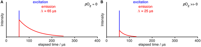
Figure 1. Illustration of a luminescence decay (A) under absence of O₂ and (B) with quenching in presence of O₂. Only a single, short impulse excitation of the luminophore (blue) and its associated luminescence decay (red) is shown.

Oxygen may quench the luminescence of the excited state L* by collision with the luminophore and transfer of the excess energy, which is called dynamic quenching¹:

$\begin{array}{ll}{\text{L}}^{\ast }+{\text{O}}_2\to \text{ L }+{\text{O}}_2^{*}.& (1)\end{array}$

This pathway of radiationless relaxation reduces both the luminescence intensity I and lifetime Λ in the presence of O₂ (Figure 1B). The amount of quenching can be related to the Stern-Volmer equation,

$\begin{array}{ll}\frac{I_0}{I}=\frac{{\Lambda }_0}{\Lambda }=1+K_{\text{SV}}^{{}^{\prime }}·a_{{\text{O}}_2}^M\approx 1+K_{\text{SV}}^{{}^{\prime }}·c_{{\text{O}}_2}^M,& (2)\end{array}$

where $K_{\text{SV}}^{\prime }$ is the Stern-Volmer constant and $a_{{\text{O}}_2}^M$ or $c_{{\text{O}}_2}^M$ are the oxygen activity or concentration, respectively, within the sensing foil containing the immobilized luminophore (^M). Oxygen behaves near-ideal, so that its (thermodynamic) activity can be replaced by its concentration. The Stern-Volmer constant is proportional to the diffusivity of oxygen, i.e., dynamic quenching is diffusion controlled (Smoluchowski equation, e.g., Lakowicz, 2006, chap. 8).

Since the equilibrium between sensing foil and ambient seawater is established via equal partial pressures pO₂ (see below), and the O₂ solubility $c_{{\text{O}}_2}^{*,M}$ within the sensing foil is generally unknown, the latter can be included in $K_{\text{SV}}=K_{\text{SV}}^{\prime }·c_{{\text{O}}_2}^{*,M}$ and Equation 2) altered to:

$\begin{array}{ll}\frac{I_0}{I}=\frac{{\Lambda }_0}{\Lambda }=1+K_{\text{SV}}·p{\text{O}}_2.& (3)\end{array}$

Note that, except for potential secondary reactions of the excited ${\text{O}}_2^{*}$ molecules, quenching does not consume any oxygen and optodes therefore do not need to be in a pumped water stream that would continuously replace any consumed oxygen in order to reach a stable (and correct) signal. Steady-state is reached when partial pressures, pO₂, are equilibrated throughout the system.

2.2. Sensor Implementation

Luminescence intensity measurements are easily biased by changes in the excitation light source intensity, ambient scattering, and other matrix effects and thus, are prone to enhanced variability and drift. Therefore, all optical oxygen sensors used in marine science measure the luminescence lifetime Λ rather than its intensity I, using a single-frequency phase shift technique: Instead of using a short pulse (compare Figure 1), the excitation is intensity-modulated. The emission is modulated with the same frequency but, due to the finite lifetime Λ of the excited state, phase shifted relative to the excitation (Figure 2). For exponential luminescence decays, the lifetime Λ is proportional to the tangent of the phase shift φ with f being the modulation frequency (Equation 4; derivation given in Lakowicz, 2006, chap. 5). Aanderaa optodes use a modulation frequency f of 5,000 Hz, while Sea-Bird optodes use 3,840 Hz.

$\begin{array}{ll}\tan \phi =2\pi ·\text{ f }·\Lambda & (4)\end{array}$

FIGURE 2

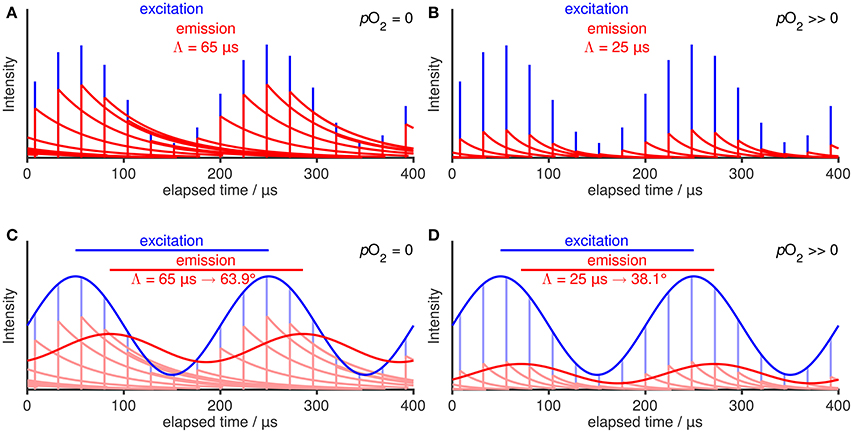
Figure 2. Illustration of luminescence decay, quenching, and phase shift lifetime measurement under absence of O₂ (left column) and presence of O₂ (right column), respectively. Conceptual addition of many intensity-modulated excitation pulses (A,B) and superposition of the luminescence decays leads to an intensity-modulated and phase shifted emission in the continuous case (C,D). The phase shift φ depends on the lifetime Λ according to Equation (4).

Thus phase shift φ and lifetime Λ carry the same information, but they are not equal. The Stern-Volmer equation is not valid for phase shifts φ (Equations 2, 3).

The luminophore in oxygen optodes is immersed and immobilized in an oxygen-permeable sensing foil or thin film, to avoid leaching of the luminophore to the environment and maintain O₂ sensitivity. The sensing foil is placed on the waterside of an optical window and thus exposed to ambient seawater, while the excitation and detection electronics are inside the sensor housing behind the optical window. Sensors are built both for unpumped (e.g., Aanderaa, JFE Advantech, RBR, Contros) and pumped (e.g., Sea-Bird) mode of operation (which does not prevent, of course, unpumped sensors to be used in a pumped flow cell).

When luminophores are dissolved in solution, the high molecular diffusivity ensures that every luminophore has the same environment on timescales of the luminescence lifetime (tens of μs). Consequently, luminophores in solution show linear Stern-Volmer behavior according to Equations (2, 3) (i.e., the ratio of I₀ to I or Λ₀ to Λ is linear with O₂). Note that even for linear Stern-Volmer behavior, the I—oxygen and Λ—oxygen relation is non-linear (Equations 2, 3; Figure 3B).

FIGURE 3

Figure 3. Conceptual illustration of linear Stern-Volmer behavior (gray) and non-linear Stern-Volmer behavior (red) as Stern-Volmer plot (A) and as plot of lifetime Λ against O₂ (B). Note that the lifetime (or phase shift)—oxygen dependency is always non-linear.

However, in condensed media such as the sensing foil of oxygen optodes, molecular motion is highly hindered. Thus, different or non-uniform chemical environments around luminophores persist on timescales of the luminescence (tens of μs), i.e., interactions with the matrix are different between luminophores. Because of this heterogeneity, all oxygen optodes show a non-linear Stern-Volmer behavior, i.e., they do not follow Equations 2, 3. Instead, they show a downward curvature of the Stern-Volmer plot (Figure 3).

Oxygen sensing with oxygen optodes imperatively require establishment of chemical equilibrium between the sensing foil, where the luminophore is immobilized, and the ambient seawater. The luminophore responds to the O₂ (thermodynamic) activity in the sensing foil $a_{{\text{O}}_2}^M$ (since quenching is diffusion-controlled), while the O₂ activity in the ambient medium, $a_{{\text{O}}_2}^L$, usually is the quantity of interest to the user. Both phases are in equilibrium when their chemical potentials are equal, i.e., ${\mu }_{O_2}^M={\mu }_{O_2}^L$. For a gas dissolved in another medium (i.e., oxygen dissolved in the sensing foil or seawater), Henry's law definition relates the chemical potential of O₂, μ_O2, to the solute's activity, a_O2, according to Equation (5) (see textbooks of physical chemistry)

$\begin{array}{ll}{\mu }_{{\text{O}}_2}={\mu }_{{\text{O}}_2}^{\circ }(T,P)+\text{R }·T·\text{ ln}\frac{a_{{\text{O}}_2}}{1\text{ mol }{\text{L}}^{-1}},& (5)\end{array}$

where ${\mu }_{O_2}^{\circ }(T,P)$ is the chemical potential of an imagined standard state at temperature T and hydrostatic pressure P with an O₂ activity of 1 mol L⁻¹ and dissolved oxygen behaving as if infinitely diluted. This standard state is specific to the medium, i.e., ${\mu }_{O_2}^{\circ ,M}\ne {\mu }_{O_2}^{\circ ,L}$. For oxygen in the gas phase, the chemical potential is given by Raoult's law,

$\begin{array}{ll}{\mu }_{{\text{O}}_2}={\mu }_{{\text{O}}_2}^{⦵}(T,P)+\text{R }·T·\text{ ln}\frac{f_{{\text{O}}_2}}{1\text{ bar}},& (6)\end{array}$

where ${\mu }_{{\text{O}}_2}^{⦵}(T,P)$ is the chemical potential of the pure gas at 1 bar (and at temperature T and hydrostatic pressure P) as standard state and f_O2 is the fugacity of O₂. Using the definition of the Henry constant, K_H,O2, or solubility, $c_{{\text{O}}_2}^{*}$, respectively,

$\begin{array}{ll}{K}_{H,{\text{O}}_2}=\frac{f_{{\text{O}}_2}}{a_{{\text{O}}_2}}=\frac{1}{c_{{\text{O}}_2}^{*}},& (7)\end{array}$

the standard potentials of Equations (5, 6) can be related,

$\begin{array}{ll}{\mu }_{{\text{O}}_2}^{\circ }(T,P)={\mu }_{{\text{O}}_2}^{⦵}(T,P)+\text{R }·T·\text{ ln }{K}_{H,{\text{O}}_2}={\mu }_{{\text{O}}_2}^{⦵}(T,P)-\text{R }·T·\text{ ln }{c}_{{\text{O}}_2}^{*}.& (8)\end{array}$

For the equilibrium condition between sensing foil and ambient medium, ${\mu }_{O_2}^M={\mu }_{O_2}^L$, we can now write

$\begin{array}{ll}{\mu }_{{\text{O}}_2}^{\circ ,M}(T,P)+\text{R}·T·\text{ ln }\frac{a_{{\text{O}}_2}^M}{1\text{ mol }{\text{L}}^{-1}}={\mu }_{{\text{O}}_2}^{\circ ,L}(T,P)+\text{R }·T·\text{ ln }\frac{a_{{\text{O}}_2}^L}{1\text{ mol }{\text{L}}^{-1}},& (9)\end{array}$

which is equal to

$\begin{array}{ll}{\mu }_{{\text{O}}_2}^{⦵}(T,P)+\text{R }·T·\text{ ln }\frac{f_{{\text{O}}_2}^M}{1\text{ bar}}={\mu }_{{\text{O}}_2}^{⦵}(T,P)+\text{R }·T·\text{ ln }\frac{f_{{\text{O}}_2}^L}{1\text{ bar}},& (10)\end{array}$

and further simplifies to equal fugacities,

$\begin{array}{ll}{f}_{{\text{O}}_2}^M=f_{{\text{O}}_2}^L,& (11)\end{array}$

as condition for the phase equilibrium between sensing foil and ambient medium. Since dissolved oxygen behaves near-ideal, activity and fugacity can be replaced by concentration and partial pressure.

In summary, while the sensing principle (luminescence quenching) is a diffusion-controlled process and thus sensitive to the oxygen concentration (again: within the sensing foil), the phase equilibrium between sensing foil and ambient medium renders oxygen optodes, in effect, sensitive to the ambient medium's partial pressure, pO₂. This has important implications for the behavior of oxygen optodes with respect to environmental factors (section 3).

Most studies to characterize oxygen optode behavior for oceanographic applications employed Aanderaa or Sea-Bird optodes, which both use the same silicone-based sensing membrane (PSt3 membrane, PreSens, Regensburg, Germany). Other manufacturers (e.g., JFE Advantech, Contros) use different sensing materials, which are both newer and less well-characterized. In addition, Aanderaa recently started to offer oxygen optodes for shallow water applications with a different membrane (WTW, Weilheim, Germany). Where available, we added preliminary information on these sensors/membranes, but in general focus on the much better studied PSt3 membrane optodes.

3. Environmental Factors

3.1. O₂ and Temperature Dependence

Oxygen decreases the luminescence lifetime Λ due to quenching. The relative change ∂Λ/∂O₂ is largest at small O₂ levels, i.e., oxygen optodes are most sensitive at low O₂ (Figures 3B, 4B).

FIGURE 4

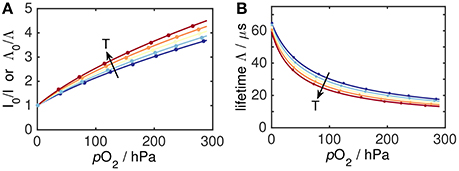
Figure 4. Optode oxygen and temperature dependence (blue–cold, red–warm) as Stern-Volmer plot (A) and as plot of lifetime Λ against O₂ (B). Dots indicate the location of actual optode calibration data at 1, 8, 15, 22, and 30 °C.

An increase in temperature reduces the lifetime of the excited state, L*, i.e., both Λ₀ and Λ are reduced (Figure 4B). Moreover, a temperature increase causes oxygen diffusivity to increase and luminescence quenching as a diffusion-controlled process becomes more efficient. In parallel, higher temperature decreases the O₂ solubility, which reduces quenching. The overall effect of these partially counteractive influences, however, is an increase in quenching and a reduction of lifetime with rising temperatures (Figure 4A). These principles are universal for all oxygen optodes.

The characterization of the combined oxygen and temperature response of optodes is the field of classical laboratory calibration. In principle, such calibration setups (e.g., Tengberg et al., 2006; Bittig et al., 2012; Bushinsky and Emerson, 2013) systematically vary oxygen and temperature over adequate ranges while monitoring the optode response (phase shift or lifetime), typically using between 5–10 oxygen and 4–7 temperature levels. A calibration matrix (O₂, T, φ) obtained in this way can then be approximated by a mathematical model ${F}$ of optode O₂–T–response of choice, that provides a mapping according to:

$\begin{array}{ll}{\text{O}}_2\leftarrow {F}(T,\phi ).& (12)\end{array}$

A variety of mathematical models exist with a common goal to provide an adequate mathematical description of the mapping function ${F}$. These models include high-order polynomials (e.g., Aanderaa Data Instruments AS, 2009, Appendix 6), parametric models inspired by Stern-Volmer (Uchida et al., 2008, 2010; Sea-Bird Electronics, 2013; this work), and two-site physics (McNeil and D'Asaro, 2014). Their output can either be an oxygen concentration c_O2 (Uchida et al., 2008; Aanderaa Data Instruments AS, 2009; Sea-Bird Electronics, 2013) or an oxygen partial pressure pO₂ (Bittig et al., 2012; McNeil and D'Asaro, 2014; this work), which both can be converted using temperature and salinity (Bittig et al., 2016). More details about these calculations can be found in section 5.2.

3.2. Salinity Dependence

The luminophore is immersed in a sensing membrane, e.g., a hydrophobic silicone matrix (PSt3 membrane) for Aanderaa and Sea-Bird optodes. Only gases (dissolved N₂, O₂, and water vapor) and no salts can penetrate into the membrane, i.e., the oxygen solubility within the sensing foil, $c_{{\text{O}}_2}^{*,M}(T)$, is independent of salinity. Thus, the optode response at a given partial pressure, pO₂, is unaffected by salinity. However, seawater oxygen solubility, $c_{{\text{O}}_2}^{*,L}(T,S)$, is a function of salinity. Therefore, the conversion between equilibrium partial pressure, pO₂ (i.e., the property which among temperature and pressure determines the O₂ activity in the foil), and seawater O₂ concentration, $c_{{\text{O}}_2}^L$, depends on the seawater salinity. This applies to all oxygen optodes.

Since most optodes² do not report partial pressure (which requires no salinity correction) but convert sensor output into O₂ concentration in seawater, a “salinity correction” of the reported concentration is necessary. This correction does not correct the optode sensor response, but simply converts O₂ partial pressure, pO₂, to seawater O₂ concentration, $c_{{\text{O}}_2}^L$. We advise to use the SCOR WG142 recommendations on O₂ quantity conversions for this step (Bittig et al., 2016). They apply the Benson and Krause refit of Garcia and Gordon (1992) for the O₂ solubility and also account for the change in atmospheric composition at different salinities (see also section 5.2.3), which is generally neglected in the manufacturer's recommendations.

3.3. Hydrostatic Pressure Dependence

Oxygen optodes show a pressure effect that is the result of three factors, which are discussed one by one below: the stability of the luminophore's excited state L* itself, the O₂ activity inside the sensing foil, and the pressure response of luminescence quenching.

The luminophore's excited state, L*, is slightly destabilized at higher pressure with respect to the ground state, L, which can be seen in experiments at low O₂ levels (e.g., Bittig et al., 2015a). The reduction in L* stability and thus a decrease in Λ₀ causes an apparent positive O₂ shift in the sensor response, independent whether O₂ is present, i.e., luminescence is quenched, or not.

The most dominant effect originates from a decrease in the sensing foil O₂ activity with pressure caused by the pressure dependence of the chemical potential. From the fundamental thermodynamic relation (definition of the Gibbs energy), pressure affects the chemical potential, μ_O2, according to:

$\begin{array}{ll}{\left(\frac{\partial {\mu }_{{\text{O}}_2}}{\partial P}\right)}_T=V_{\text{m},{\text{O}}_2},& (13)\end{array}$

where V_m,O2 is the partial molar volume of O₂, i.e., pressure increases the chemical potential μ_O2. As illustrated in Ludwig and Macdonald (2005), the concentration (and activity) stays nearly unchanged upon pressurization and the main pressure effect is on the chemical potential of the reference state, ${\mu }_{{\text{O}}_2}^{\circ }(T,P)$ (see case i, Ludwig and Macdonald, 2005, and compare Equation 5). As a consequence, solubility changes with pressure (e.g., Taylor, 1978). The change in ${\mu }_{{\text{O}}_2}^{°}$ and solubility $c_{{\text{O}}_2}^{*}$ accounts for the structural effect of pressure (on solute–solvent and solvent–solvent interactions).

This results in a higher outgassing tendency of O₂ with pressure (i.e., an increased pO₂) both in the sensing membrane and in seawater following

$\begin{array}{ll}p{\text{O}}_2(P)=p{\text{O}}_2(P_0)·\exp \left(\frac{V_{\text{m},{\text{O}}_2}·(P-P_0)}{\text{R }·T}\right).& (14)\end{array}$

Experimentally, Enns et al. (1965) found a 14 % per 1,000 dbar increase of pO₂ in seawater, which corresponds to a partial molar volume $V_{m,{\text{O}}_2}^L$ of 31.7 mL mol⁻¹. For a silicone membrane as utilized by Aanderaa or Sea-Bird optodes, literature values for $V_{m,{\text{O}}_2}^M$ are between 39 and 46 mL mol⁻¹ (see Bittig et al., 2015a). Since the partial molar volumes and thus the pO₂ increase are different between sensing foil and ambient seawater, oxygen optodes show a pressure effect. The equilibrium condition of equal partial pressures (Equations 11) is true also upon pressurization. After some transformations of Equations (10, 14 Bittig et al., 2015a), one obtains Equation (15) for the change in membrane O₂ concentration due to a re-equilibration of O₂ between sensing foil and ambient seawater upon pressurization from P₀ to P. With $V_{m,{\text{O}}_2}^M>V_{m,{\text{O}}_2}^L$, the membrane O₂ concentration $c_{{\text{O}}_2}^M$ (and activity) decreases at higher pressures.

$\begin{array}{ll}{c}_{{\text{O}}_2}^M(P)=c_{{\text{O}}_2}^M(P_0)·\exp \left(\frac{(V_{\text{m},{\text{O}}_2}^L-V_{\text{m},{\text{O}}_2}^M)·(P-P_0)}{\text{R }·T}\right)& (15)\end{array}$

Luminescence quenching, in contrast, is mostly unaffected by pressure. This at first counterintuitive observation is because dynamic quenching by O₂ is a diffusion-controlled process (see Lakowicz, 2006). The diffusion of oxygen is driven by the gradient in chemical potential and retarded by frictional resistance. Pressure increases μ_O2 (Equation 13), however, it is shifted by the same amount throughout the entire medium (since V_m,O2 is the same throughout). Thus, the gradient of μ_O2 remains constant and quenching within the sensing foil stays the same. In fact, Carey and Gibson (1976) observed only a small increase in fluorescence intensity (5 % at 10,000 dbar) for quenching by O₂ in solution, attributed to the compression of the solution (and thus changes in the concentration).

To our knowledge, pressure experiments were only done with PSt3 membranes, but other sensing membranes can be expected to show similar effects. The pressure response of Aanderaa oxygen optodes has been studied by Tengberg et al. (2006) in the laboratory as well as by Uchida et al. (2008) in the field and more thoroughly by Bittig et al. (2015a) (both laboratory and field), also including Sea-Bird optodes. A two-fold pressure response has been observed:

i. Pressure affects the lifetime Λ₀ in the absence of O₂ with decreasing Λ₀ under pressure.

ii. Pressure affects the apparent O₂ level with sensors reporting lower O₂ levels under pressure.

The first effect (i) can be explained by a destabilization of the excited state, L*. The associated decrease in Λ₀ causes an apparent positive O₂ shift in the sensor response at all O₂ concentrations. The second effect (ii) combines the re-equilibration of O₂ levels between sensing foil and seawater as well as the pressure dependence of quenching. Its magnitude matches the decrease in PSt3 sensing membrane $c_{{\text{O}}_2}^M(P)$ due to O₂ re-equilibration: Reported O₂ levels decrease by about −4.3 % per 1,000 dbar (see section 5.2.4 or Bittig et al., 2015a) as result of a ca. 14 % per 1000 dbar increase of pO₂ in seawater and an order of 10 % per 1,000 dbar increase of pO₂ in the PSt3 silicone sensing foil (Equation 15). However, the temperature dependence of ii is inverse to the expectation (Equation 15), indicating the presence of additional effects (e.g., a small pressure dependence of quenching, Bittig et al., 2015a). Effects i and ii oppose each other, but the re-equilibration dominates the pressure response: Overall, uncorrected optode readings are biased high at O₂ levels below ca. 5 % O₂ saturation (i dominates over ii), while they are biased low above this level (ii dominates over i; Bittig et al., 2015a).

Previous studies of Aanderaa optode pressure response (Tengberg et al., 2006; Uchida et al., 2008) were unable to separate the pressure effects i and ii, which is why they report an apparently smaller O₂-pressure dependence. Results of Bittig et al. (2015a) (given in detail in section 5.2.4) are consistent with the data of Uchida et al. (2008), however, preference should be given to account for both effects separately, if possible (i.e., if optode phase shift data are available).

Pressure vessel experiments at compression / decompression rates around 10 dbar s⁻¹ showed a near-instantaneous pressure response of optodes with PSt3 membrane (within the 60 s logging interval) that was fully reversible (i.e., without hysteresis) (Bittig et al., 2015a). However, there is sporadic evidence for second-order effects not yet fully understood, e.g., Bittig and Körtzinger (2017) report on a potential pressure conditioning of optodes on two floats after repeated pressure cycling to 2000 dbar (order of 40 pressure cycles, amplitude 1–2 μmol kg⁻¹), being caused by either the Aanderaa 4330 or Sea-Bird SBE63 optode or both.

3.4. Time Dependence #1: Dynamic Time Response

The time response of oxygen optodes to a change in ambient O₂ levels is not instantaneous. This response is especially noticeable when an optode travels through a large oxygen gradient. Deepening winter mixed layers in the Gulf of Alaska form such gradients and optodes on profiling floats there can underestimate the mixed layer oxygen concentration by 5 μmol kg⁻¹ (Plant et al., 2016, Figure 6). Oxygen has to diffuse in or out of the sensing foil (^M) to reach a new equilibrium with the ambient medium (^L) (Equation 11), which causes a lag in the optode time response. The transfer of O₂ at the interface is determined by the temperature-dependent O₂ diffusivity and solubility in both phases as well as the thickness of the liquid boundary layer. Bittig et al. (2014) developed a simple one dimensional diffusion model that accounts for the temperature dependence of O₂ diffusivity and solubility in both phases but simplifies the liquid boundary layer to a stagnant boundary layer with only molecular diffusion.

The model helps to conceptually understand the processes which are responsible for the dynamic time response of optodes. The response from an equilibrated state with equal partial pressure throughout the system (normalized partial pressure Φ(x≥0, t = 0⁻) = 0) to a step-change in ambient partial pressure (normalized partial pressure $\Phi (x\ge l_M+l_L,t=0^{+})=1$) is shown in Figure 5A for a silicone membrane with a thickness l_M of 100 μm (Aanderaa optode standard foil) and a stagnant boundary layer thickness l_L of 60 μm, where x is the distance from the optical window. The change in ambient O₂ level has first to diffuse into the boundary layer until a change in sensing foil O₂ is noticeable. Then, the change in sensing foil O₂ levels in response to the change in ambient O₂ is limited by the transfer through the boundary layer. The thicker the boundary layer, the slower the oxygen response of the optode and vice versa (Figure 5B).

FIGURE 5

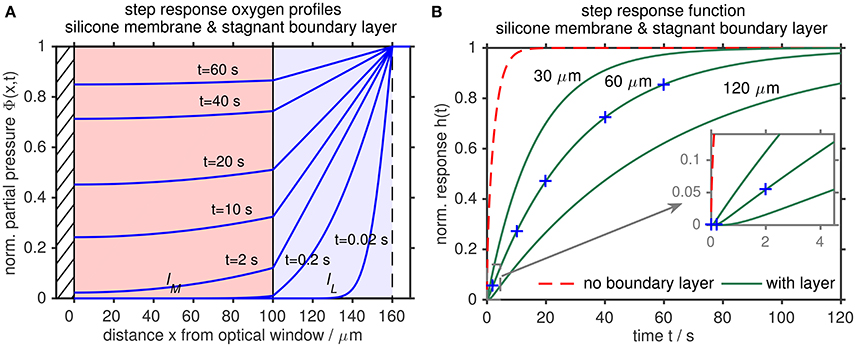
Figure 5. Stagnant boundary layer diffusional model of an O₂ optode to a step change in ambient O₂ levels at 25 °C. The optode consists of a silicone membrane (0≤ x≤ l_M, l_M = 100 μm, Aanderaa optode standard foil, pale red) with impermeable boundary (optical window, hatched) on one side and a stagnant liquid boundary layer (l_M≤x≤(l_M+l_L), l_L = 60 μm, pale blue) on the other side. (A) Normalized partial pressure response inside the two layers: O₂ has first to diffuse through the boundary layer to change O₂ levels inside the sensing foil, which limits the optode time response. (B) Normalized O₂ step response function h(t) for different boundary layer thicknesses l_L (green) and for a gas phase time response without liquid boundary layer (l_L = 0 μm, dashed red) (after Bittig et al., 2014).

Bittig et al. (2014) found that temperature modifies the response time τ, but does not affect the modeled boundary layer thickness l_L. This should be valid for all oxygen optodes. Moreover, they provide a lookup table for response times τ as function of temperature T and l_L for PSt3 membranes with different membrane thickness l_M (see Supplemental Material of Bittig and Körtzinger, 2017; Figure S2 of this work).

The modeled boundary layer thickness l_L, in turn, is determined by the flow in front of the sensing foil (Bittig et al., 2014): High flow speeds erode/renew the boundary layer more efficiently, leading to a faster O₂ transport through the boundary layer and thus shorter response times τ, and vice versa. From laboratory experiments with PSt3 membrane optodes, Bittig et al. (2014) observed an inverse relation between boundary layer thickness l_L and flow $\stackrel{.}{V}$ for pumped applications following

$\begin{array}{ll}{l}_L(\text{pumped})/\mu \text{m}=1.8·{10}^4·\frac{1}{\dot{V}/\text{mL }{\text{min}}^{-1}}+4& (16)\end{array}$

with an uncertainty of 4 μm or 10 %, whichever is greater (Bittig and Körtzinger, 2017, Appendix A). For unpumped applications, the relation between l_L and platform velocity must be established on a case-by-case basis depending on the platform characteristics and optode attachment with respect to flow direction. For typical Biogeochemical-Argo profiling floats, Bittig and Körtzinger (2017) give a characterization for PSt3 membranes following:

$\begin{array}{ll}{l}_L(\text{float})/\mu \text{m}=\{\begin{array}{ll}210-\frac{110}{0.095}·\left|\upsilon /\text{dbar }{\text{s}}^{-1}\right|\hfill & \left|\upsilon \right|\le 0.095\text{ dbar }{\text{s}}^{-1}\hfill \\ \begin{array}{l}20+\frac{80}{0.905}·\left(1-\left|\upsilon /\text{dbar }{\text{s}}^{-1}\right|\right)\hfill \end{array}\hfill & \left|\upsilon \right|>0.095\text{ dbar }{\text{s}}^{-1}\hfill \end{array},& (17)\end{array}$

where υ is the ascent velocity of the float. The two regimes likely correspond to the shift between laminar and turbulent flow at the sensing foil (Bittig and Körtzinger, 2017) that is not covered by the simple stagnant boundary layer model of Bittig et al. (2014).

Observed boundary layer thicknesses l_L for unpumped Aanderaa optodes translate for the standard PSt3 foils to response times τ on the order of 15–45 s for shipboard CTD applications (Bittig et al., 2014) and of 70–140 s for profiling floats (Bittig and Körtzinger, 2017), depending on flow and temperature. For the Aanderaa fast-response foil, which is a thinner PSt3 foil and without black optical isolation, the corresponding ranges are 8–25 and 35–70 s, respectively. However, there are few oceanographic field data with fast-response foils to support these estimates. Boundary layer thicknesses l_L for pumped Sea-Bird optodes translate to response times τ between 6 and 15 s on a shipboard CTD (flow ca. 7,000 mL min⁻¹) and between 25 and 40 s on a moored or Argo CTD (flow ca. 600 mL min⁻¹), depending on temperature. An unpumped RINKO optode by JFE Advantech showed response times τ between 3 and 7 s on a shipboard CTD during a polar deployment (i.e., cold temperatures with slow time response; Bittig et al., 2014). Preliminary results from a Contros Hydroflash O₂ optode indicate a time response comparable to the Aanderaa fast-response foil or slightly faster (T. Hahn, GEOMAR, pers. comm.).

The estimate of τ can then be used to inverse-filter and correct observations by appropriate algorithms. Care must be taken not to excessively amplify noise. One possible correction algorithm is presented in Bittig and Körtzinger (2017, Appendix A) and Bittig et al. (2014) (reproduced in the Supplementary Material), while Fiedler et al. (2013) used the algorithm of Miloshevich et al. (2004). An example is given in Figure S3 for one CTD and one profiling float profile (after Bittig et al., 2014; Bittig and Körtzinger, 2017).

A time response correction provides a-priori a more accurate estimate of the “true” O₂. However, the impact of the correction strongly depends on the O₂ profile / gradient and response time (and thus on flow). For an unpumped Aanderaa optode mounted on a CTD, Bittig et al. (2014) observed differences between negligible to more than 50 μmol kg⁻¹ between observed and time response corrected O₂ (validated against reference CTD-O₂; see Figure S3a). On a profiling float, median differences between observed and corrected O₂ were between 13 and 15 μmol kg⁻¹ for an unpumped Aanderaa optode and between 6 and 7 μmol kg⁻¹ for a pumped Sea-Bird optode, respectively, in the strongest O₂ gradients (120 μmol kg⁻¹ change over 8 min or 20 dbar). After correction, both sensors agreed to within 2–3 μmol kg⁻¹ (Bittig and Körtzinger, 2017).

In any case, a correction of the dynamic time response works on a time axis and thus requires time stamps for optode samples. These need to be acquired and stored alongside the optode data.

3.5. Time Dependence #2: Sensor O₂-Response Drift

Oxygen optodes with PSt3 foils have been documented to be considerably out of calibration compared to field data (e.g., Takeshita et al., 2013, mean bias of −5.0 % O₂ saturation at 100 % O₂ saturation for 130 Aanderaa optodes). This has been puzzling since field deployments of oxygen optodes indicated high stability in-situ (e.g., Körtzinger et al., 2005; Tengberg et al., 2006). Indeed, there appear to be two distinct regimes: (1) storage regime, i.e., before and/or between deployments, and (2) deployment regime, i.e., when submerged continuously in seawater. When not deployed and stored in air, abundant laboratory data show that optodes can lose O₂ sensitivity on the order of 5 % per year. Given the oceanographic accuracy aim of 0.5 % O₂ saturation / 1 hPa (Gruber et al., 2010), optodes should thus be assumed to be out of calibration after having been stored or not used for a period of several months. This holds in particular for recently produced sensors, whereas old ones tend to drift less (order of 1 % per year or less). During deployments, however, optode O₂ sensitivity drift seems to be drastically reduced and optodes are “stable” within a few tenths of a percent per year. We will discuss both regimes below.

3.5.1. During Storage

3.5.1.1. Drift character

While there is abundant data in the literature of PSt3 membrane optodes showing a low bias with respect to a previous calibration, there has been some uncertainty about the nature and the character of optode O₂ sensitivity drift.

A linear O₂ dependence of the observed drift was first shown with repeated optode laboratory calibrations in Bittig et al. (2012) and later refined in Bittig and Körtzinger (2015). Bittig and Körtzinger (2015) also proposed a mechanistic explanation for the O₂ response drift, being mainly (1) due to reduced quenching of the luminophore (i.e., a reduced O₂ sensitivity), and (2) a counteracting, destabilizing effect on the luminophore itself. The first expressed itself as a factor on O₂, whereas the second manifested itself as a (positive) oxygen intercept at zero O₂. Nicholson and Feen (2017), in fact, confirm a positive zero intercept based on field data. Furthermore, Bushinsky et al. (2016), Drucker and Riser (2016), and Nicholson and Feen (2017) show that a slope correction alone might be insufficient at low O₂ levels, while it is appropriate near 100 % O₂ saturation.

In contrast to the laboratory evidence, Drucker and Riser (2016) advocate for a linear phase correction, hinting at a higher physical plausibility of a linear phase correction (i.e, changing a particular subset of calibration coefficients) compared to a linear oxygen correction (i.e., changing a different subset of calibration coefficients), which we argue to not be the case. In fact, a linear phase correction exactly creates the kind of “second-order error due to the nonlinearity of the oxygen equation” that Drucker and Riser (2016) initially wanted to avoid (see below).

To clarify the drift character of oxygen optodes, we collected the calibration data of 14 Aanderaa optodes and one Sea-Bird optode that were calibrated at least three times either at the BCCR Bergen/CSIRO-O&A Hobart (12 Aanderaa optodes with 113 calibrations), GEOMAR Kiel (4 Aanderaa optodes with 15 calibrations and 1 Sea-Bird optode with 2 calibrations), or the manufacturer facilities (1 Sea-Bird optode with 1 factory calibration). The BCCR Bergen and CSIRO-O&A Hobart setups are identical. They use a jacketed glass reactor vessel such that a circulating bath can control temperature, and N₂ and O₂ gases together with mass flow controllers to control pO₂. The GEOMAR Kiel setup uses an electrochemical generation of O₂ to control O₂ levels (Bittig et al., 2012). All calibrations were performed in freshwater. Optodes were stored at room temperature, some with and some without wetted sensing foil. Six of the CSIRO-O&A optodes had been “burnt-in” (see details in Tengberg and Hovdenes, 2014) with 5 million samples before the first calibration, whereas all other optodes did not receive a similar pre-conditioning. Optode 4330 1082 (model number serial number) received a burn-in with 1.2 million samples between its second and third calibration, whereas no record of a dedicated burn-in is available for optode 4330 0564. Between calibrations, optodes were deployed on profiling CTDs, surface underway systems in polar or tropical conditions, or kept in the laboratory at all times, i.e., the sensors were exposed to all kinds of treatments and conditions.

A subset of the calibration data for optode 3835 1451 is shown in Figure 6 (a larger subset with all sensors is given in Figure S4). Upper and lower panels show the same data, once expressed as oxygen concentration and once expressed as oxygen partial pressure (for conversions see Bittig et al., 2016).

FIGURE 6

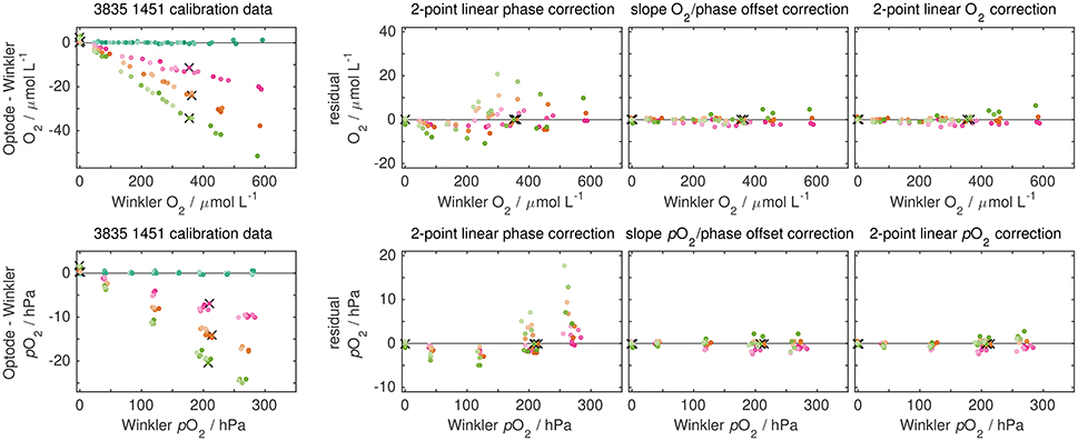
Figure 6. Character of drift (left) and comparison of correction approaches by 2-point correction (right set of panels) for a subset of calibrations of optode 3835 1451 (CSIRO-O&A, Hobart). The timing between calibrations is shown in Figure 7 with the same color code. Lighter colors indicate calibration points at lower temperatures. Upper and lower panels show the same data but either expressed as O₂ concentration or O₂ partial pressure. The first calibration was used to derive optode calibration coefficients that were applied to subsequent calibration data. Two-point corrections were mimicked by using just two specific calibration points of the calibration data (denoted by black crosses), whereas residuals after correction are shown for the full calibration data. Sensor drift is linear with oxygen and shows a small (positive) intercept at zero O₂. Accordingly, corrections with a slope O₂ concentration/partial pressure term perform well, while a linear phase correction shows significant mismatch between corrected and reference data both at different O₂ and temperatures than the 2-point data. Data for all sensors are given in Figures S4, S5.

The O₂ response drift is linear with oxygen and can reach a decrease in O₂ sensitivity on the order of −10 %. As secondary effect, a significant non-zero intercept at zero O₂ on the order of a few μmol L⁻¹ or hPa, respectively, is observed. This intercept tends to be positive, i.e., overestimating actual O₂ near zero O₂, whereas the O₂ sensitivity loss causes an underestimation elsewhere.

This behavior is similar to the optode pressure response and can be explained in the same way. As main effect, luminescence quenching by oxygen decreases. This is linearly related with the oxygen content (Equations 2, 3). It can be caused by a degraded O₂ accessibility to the luminophore (e.g., due to migration of the luminophore) or a decreased O₂ diffusivity within the sensing foil, which reduces the likelihood of collision between O₂ and luminophore molecules and thus the quenching (Bittig and Körtzinger, 2015). In parallel, the lifetime Λ₀ of the luminophore becomes smaller. Compared to initial conditions, a shorter lifetime Λ₀ is interpreted as higher presence of quencher, i.e., a positive bias in O₂. With aging or a change in the sensing foil (e.g., migration of the luminophore), the luminophore is in an energetically more favorable environment which, in turn, reduces Λ₀.

3.5.1.2. Drift correction

In practice, one often faces the situation of having available only two reference points (e.g., 0 and 100 % O₂ saturation) or reference clusters (e.g., deep and surface oxygen profile data) but not a full calibration matrix for drift correction. We therefore used our multiple calibration data to (1) derive calibration coefficients from the first calibration and (2) use the subsequent calibrations to mimic a 2-point correction (i.e., only using one calibration point near 100 % O₂ saturation and 10 °C and one at zero O₂ and 20 °C; These are typical conditions for Aanderaa factory calibration 2-point adjustments) and to use the remainder of the calibration data to assess the quality of a 2-point drift correction. Here we applied three correction approaches: a linear phase domain (Drucker and Riser, 2016), a mixed approach with a slope factor on O₂ and an offset on φ, and a linear oxygen domain correction (e.g., Takeshita et al., 2013) (Figure 6, right set of panels, for optode 3835 1451 and Figure S5 for all optodes).

A linear phase correction, as proposed by Drucker and Riser (2016), in fact creates exactly the effect the authors want to avoid, i.e., a misinterpolation and -extrapolation beyond the reference O₂ levels due to a misrepresentation of the O₂ sensitivity. This confirms that O₂ sensitivity drift should be corrected with a factor on oxygen, not phase. A slope factor on oxygen is conceptually equivalent to a slope factor on all quenching calibration coefficients (compare Equations 2, 3), no matter which mathematical model ${F}$ is used (Equation 12). It is thus not just a phenomenologic slope correction, but a physically justified recalibration. Taking into account measurements in seawater and freshwater, preference should be given to a pO₂ slope factor correction (and Equation 3), since the same O₂ concentration in freshwater and in seawater implies different partial pressures pO₂ and thus quenching of the luminescence within the sensing foil. Applying the non-zero intercept at zero O₂ either to φ, to O₂ concentration, or to pO₂ yields comparable results. The adequate location of this offset correction somewhat depends on the nature of ${F}$ (see section 5.2) and whether ${F}$ provides access to and/or a parameterization of Λ₀, which conceptually would be the adequate place.

3.5.1.3. Drift time evolution

Using three Aanderaa optodes, D'Asaro and McNeil (2013) demonstrated that the response at 100 % O₂ saturation decreases exponentially with a time constant of 1.94 years. Our multiple calibration data of PSt3 membrane optodes confirms this finding. Figure 7 shows the temporal evolution of the pO₂ slope (i.e., the loss in O₂ sensitivity) for a linear oxygen domain correction using all our calibration data. The average exponential time constant is 2.22 ± 0.57 years (all data with 95 % CI) for the 12 optodes that had at least 5 calibrations. The drift amplitude is surprisingly similar, around −6 ± 1 % total drift over the life of the optode for optodes with burn-in pre-conditioning, and around twice the amount for optodes without. The mean drift in the pO₂ zero intercept is indistinguishable from zero (data not shown).

FIGURE 7

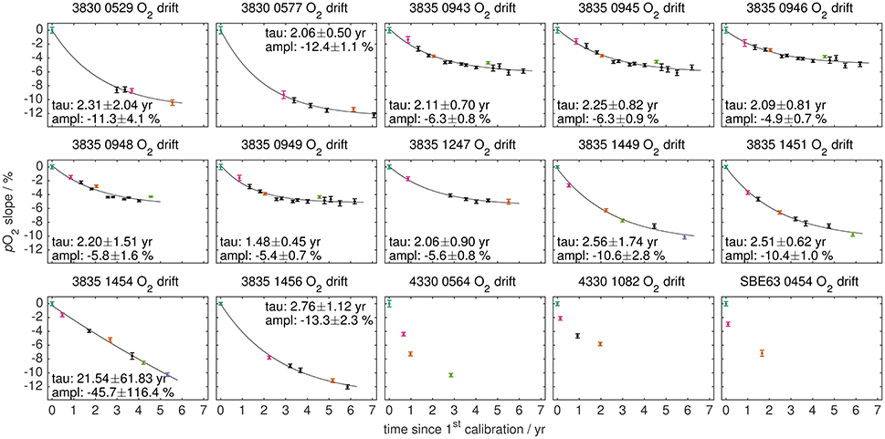
Figure 7. Oxygen sensitivity change for all optodes: The pO₂ slope factor of a linear oxygen domain correction is shown against the time elapsed since the first calibration. Exponential fits are given for optodes with at least 5 calibrations, where tau represents the exponential time constant and ampl the amplitude (both with 95 % CI). The subset of colored calibrations is shown in Figures S4, S5 with the same color code.

A side-by-side deployment of one Aanderaa optode with PSt3 foil and one with WTW foil suggests that WTW foils may be more stable. While the PSt3 foil drifted by −4.1(±0.1) % during 20 months (with repeated deployments in tropical surface waters for a total of about 1 month), the WTW foil showed a sensitivity reduction of only −1.3(±0.3) % during the same period and handling. Both sensing foils were new and had not received a burn-in. However, the drift character of the WTW foil still needs to be established (in particular whether it is uniform at all temperatures).

3.5.2. During Deployment

3.5.2.1. From Argo-O₂ float-mounted optodes

To assess stability or drift in-situ, reference data of sufficient accuracy are required. Assuming no change in O₂ in the deep Labrador Sea, Tengberg et al. (2006) detected no significant optode drift for a float timeseries of 1.6 years. As an alternative to O₂ at depth, optode in-air measurements were proposed by Körtzinger et al. (2005) and first used for calibration by Fiedler et al. (2013). Their operational potential to calibrate optodes was demonstrated subsequently by Bittig and Körtzinger (2015), Johnson et al. (2015), and Bushinsky et al. (2016) on floats and more recently also on gliders (Nicholson and Feen, 2017).

From the literature, evidence for optode drift or stability has been mixed: Bittig and Körtzinger (2015) detected no significant drift over 15 months of float data, which they revised in Bittig and Körtzinger (2017) with a longer float timeseries. After 3 and 2 years, respectively, they observed a significant O₂ sensitivity loss of −0.40 and −0.27 % year⁻¹ for two floats. Johnson et al. (2015) obtained both significant positive and negative drift for a fleet of 29 floats with a range of −0.9 to +1.3 % year⁻¹ and an insignificant mean of +0.2 % year⁻¹, from which they concluded that optodes are stable in-situ on average. Finally, Bushinsky et al. (2016) reported a significant optode drift for 10–12 out of 14 optodes with both positive and negative drift and a significant mean trend of −0.12 % year⁻¹.

Methods of data analysis as well as implementation of the measurement routine are slightly different between these studies. Therefore, we revisited the data from all floats known to us that performed in-air measurements. This includes the extended timeseries of floats from Bittig and Körtzinger (2015), Bushinsky et al. (2016), and from Johnson et al. (2015). Interpretation of data was limited to floats that had at least two years of data. Float 4900883 was excluded because (1) in air data reflected to almost 90 % in water samples and (2) suspected optode malfunctioning started 1.5 years after deployment. This leaves a total of 67 floats, of which 15 have an individual multi-point laboratory calibration and 52 have only the factory batch calibration. Out of the 67 floats, the 13 SOS-Argo floats (denoted “Emerson”) are notably different, since their optodes were attached on a 61 cm long stick, whereas the optode stick length was between 10 and 25 cm for the other floats (see float configurations given in Table S1).

3.5.2.1.1. In-air measurements: Principle

Optode surface “in air” measurements, pO_2,surf, represent a mixture of the properties of pure air, pO_2,air, and pure water, pO_2,water, which has been described as water-side “carry-over” effect (Bittig and Körtzinger, 2015; Johnson et al., 2015). It is speculated that the carry-over is due to the optode being regularly re-submerged during surface measurements, causing the air-measurements to be more or less biased toward the water-side pO_2,water, and that its magnitude is related to the height of the optode above the sea surface (as well as sea state and resulting frequency of submergence). The effect is parameterized with the carry-over slope c as a function of surface water supersaturation according to

$\begin{array}{ll}p{\text{O}}_{2,\text{surf}}-p{\text{O}}_{2,\text{air}}=c·\left(p{\text{O}}_{2,\text{water}}-p{\text{O}}_{2,\text{air}}\right).& (18)\end{array}$

While pO_2,water can be derived from near-surface in-water optode measurements, pO_2,air must be calculated from meteorological or reanalysis data,

$\begin{array}{ll}p{\text{O}}_{2,\text{air}}={\chi }_{{\text{O}}_2}·\left(p_{\text{air}}-x·p{\text{H}}_2\text{O}(T,S)\right),\text{ with }{\chi }_{{\text{O}}_2}=0.20946,& (19)\end{array}$

where p_air is the sea level air pressure, χ_O2 the mole fraction of O₂ in dry air, pH₂O(T, S) the water vapor pressure at the sea surface, and x a scaling factor (0 …1) depending on the relative humidity at the optode during in-air measurements (e.g., Bittig and Körtzinger, 2015). For the present analysis, let us neglect a potential daytime dependence of the surface measurements as evidenced in the literature (Bushinsky et al., 2016; Bittig and Körtzinger, 2017).

Considering the optode drift character (section 3.5.1.1), in air measurements only provide one O₂ reference cluster near 100 % O₂ saturation, i.e., only a 1-degrees of freedom correction of in-situ $p{\text{O}}_2^{\text{obs}}$ is possible in O₂-space using an oxygen slope m,

$\begin{array}{ll}p{\text{O}}_2=m·p{\text{O}}_2^{\text{obs}}.& (20)\end{array}$

With Equation (18) this gives

$\begin{array}{ll}m·p{\text{O}}_{2,\text{surf}}^{\text{obs}}-p{\text{O}}_{2,\text{air}}=c·\left(m·p{\text{O}}_{2,\text{water}}^{\text{obs}}-p{\text{O}}_{2,\text{air}}\right),& (21)\end{array}$

which can be rearranged to solve for the two unknowns, the carry over slope c and the oxygen slope m (see Bittig and Körtzinger, 2015).

Preliminary analysis showed that there might be some inaccuracy in the 52 factory batch calibrations, which adjusted a batch foil characterization to the individual optode using only data at two points, 20 °C and 0 % O₂ saturation as well as 10 °C and 100 % O₂ saturation. To determine whether this is the case, we added another parameter: By assuming that our O₂-T-response near saturation is only valid at 10 °C (where it was adjusted) and that we have a linear offset in pO₂ the farther we diverge from 10 °C (see example in Figure S6), we can approximate that offset with a pO₂-T-slope a according to:

$\begin{array}{ll}p{\text{O}}_2=m·\left(p{\text{O}}_2^{\text{obs}}+a·(\vartheta -{10}^{°}\text{C})\right).& (22)\end{array}$

This equals a two degrees of freedom correction of $p{\text{O}}_2^{\text{obs}}$ in O₂-T-space (compare Equation 20), and the pO₂-T-slope a corresponds to a mis-calibration of the T-response around 100 % O₂ saturation for the temperatures encountered by the float. With Equation (18) this gives

$\begin{array}{ll}\begin{array}{l}m·(p{\text{O}}_{2,\text{surf}}^{\text{obs}}+a·({\vartheta }_{\text{surf}}-10{}^{°}\text{C}))-p{\text{O}}_{2,\text{air}}\\ =c·(m·\left(p{\text{O}}_{2,\text{water}}^{\text{obs}}+a·({\vartheta }_{\text{water}}-10{}^{°}\text{C})\right)\\ -p{\text{O}}_{2,\text{air}}),\end{array}& (23)\end{array}$

which can be rearranged to

$\begin{array}{l}\begin{array}{l}p{\text{O}}_{2,\text{surf}}^{\text{obs}}=c·\left(p{\text{O}}_{2,\text{water}}^{\text{obs}}+a·({\vartheta }_{\text{water}}-10{}^{°}\text{C})\right)\\ +\frac{1-c}{m}·p{\text{O}}_{2,\text{air}}-a·({\vartheta }_{\text{surf}}-10{}^{°}\text{C}).\end{array}\end{array}$

We use Equation (23) to analyze each float timeseries and solve for the three unknowns, the carry over slope c, the oxygen slope m, and the pO₂-T-slope a at 100 % O₂ saturation. Subsequently, we use the parameters c and a from the whole timeseries to estimate an oxygen slope m_i for each surfacing i. This timeseries was analyzed for a linear trend in 1/m_i (to be consistent with Johnson et al., 2015). For comparison, we performed the same analysis with Equation (21).

Figure 8 and Table S2 give the results for the 15 optodes with individual multi-point laboratory calibration, while Figure 9 and Table S3 show the results for the 52 optodes with only factory batch calibration. In-air observation time series as well as carry-over plots (compare Equation 18) for a subset of floats are shown in Figures S7, S8.

FIGURE 8

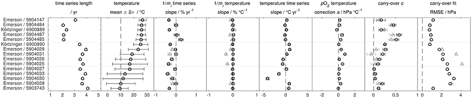
Figure 8. Results of the in air analysis according to Equation (21) (gray triangles; $\text{without }p{\text{O}}_{\text{2}}-T\text{ slope }a$) and (23) (black circles; with pO₂-T slope a) for optodes with individual multi-point laboratory calibration. Results between both approaches are very similar. The pO₂-T corrections a are near zero, indicating a proper O₂-T-response around 100 % O₂ saturation. Error bars give the 95 % confidence interval. All optodes are Aanderaa 4330 models.

FIGURE 9

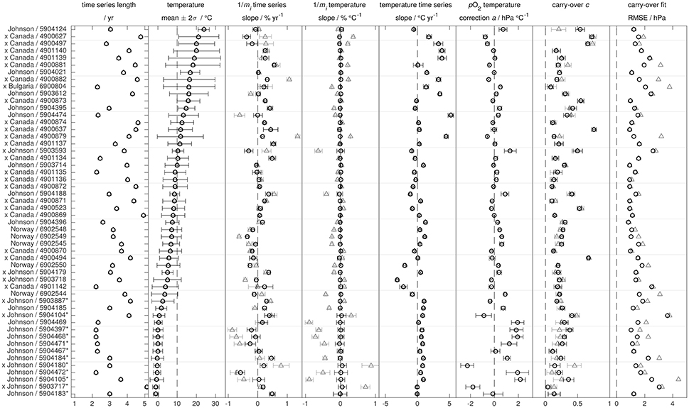
Figure 9. Results of the in air analysis according to Equation (21) (gray triangles; $\text{without }p{\text{O}}_{\text{2}}-T\text{ slope }a$ a) and (23) (black circles; with pO₂-T slope a) for optodes with factory batch calibration. Error bars give the 95 % confidence interval. Floats with Aanderaa 3830 optodes are marked with an x whereas all other floats carry an Aanderaa 4330 optode. Floats intermittently operating under sea ice are denoted by an asterisk.

3.5.2.1.2. In-air measurements: Data

For the 15 floats with individual multi-point calibration, only 3 floats show a different trend in the timeseries of the oxygen slope between Equations (21, 23) (maximum difference of 0.3 % year⁻¹). Only one float shows a significant positive drift in the O₂ sensitivity (95 % CI) while 11 (after Equation 21) or 8 (after Equation 23) show a significant negative drift to lower O₂ sensitivity with an overall range of −0.4 to +0.2 % year⁻¹. The mean (±2 standard deviations) drift rate is −0.16 (±0.39) % year⁻¹ for the 15 individually calibrated optodes (after Equation 23). Moreover, pO₂-T-slopes a are close to zero and the quality of the fit (assessed by the root mean squared error, RMSE) is comparable between Equations (21, 23) (Figure 8). This suggests (1) robustness of our analysis, (2) in general adequacy of the individual multi-point calibrations to represent the O₂-T-response, and (3) no bias or overfitting introduced by the extra parameter a for well-calibrated optodes.

For batch factory calibrated optodes, inclusion of the pO₂-T-slope a (Equation 23) significantly improves the quality of the fit (lower RMSE) compared to Equation (21) both at low and high surface temperatures (i.e., away from 10 °C), while the effect at 10 °C is near marginal (Figure 9 and Table S3). In particular for floats deployed at near-zero temperatures (i.e., at the edge of the factory calibration data where the lowest temperature is 3 °C), pO₂-T-slopes a are large. This implies that the batch factory calibration procedure, in particular its two-point adjustment (refit a, see section 4.2.1.1), is insufficient to represent the temperature behavior at 100 % O₂ saturation, i.e., insufficient to adjust the O₂-T-response to the individual optode. This is further corroborated by re-doing the analysis with a different batch calibration adjustment (refit e, see section 4.2.1.1; data not shown), which somewhat reduces the magnitude of a but does not affect neither m nor c. To avoid such an insufficient calibration of the O₂-T optode response, it is thus advisable to only use optodes with an individual multi-point calibration.

A misadjusted O₂-T-response can create spurious effects on the time series of oxygen slopes 1/m_i: If oxygen measurements are not T-compensated adequately when the float experiences a change in temperature, it creates an apparent bias in the oxygen gain. This apparent correlation (compare Johnson et al., 2017) is avoided by using Equation 23 including the additional pO₂-T-slope a, which, in practice, eliminates any gain m_i temperature dependence observed after Equation (21) (Figure 9 and Table S3). Inclusion of a significantly reduces the range of apparent drifts from −0.9 to +1.4 % year⁻¹ (after eq. 21, see Johnson et al., 2017) to a more realistic −0.6 to +0.6 % year⁻¹ (after Equation 23) by decoupling the oxygen slope time series from the temporal evolution in temperature. For this reason, we focus on the results following Equation (23).

Nonetheless, the range of drift rates is about twice as large as for floats with individual multi-point calibration, which may be related to the higher uncertainty in the O₂-T-response characterization (including the pO₂-T-slope a) for factory batch calibration. Of the 52 factory batch calibrated optodes, 27 show a significant positive drift (95 % CI) and 14 a significant negative drift to lower O₂ sensitivity (after Equation 23). The mean (±2 standard deviations) drift rate is +0.09 (±0.53) % year⁻¹ for the 52 factory batch calibrated optodes, and +0.04 (±0.54) % year⁻¹ for all 67 floats combined (after Equation 23).

In addition, we see a somewhat larger range (0.01 − 0.76) for the carry-over slope c in our analysis than previously reported, whereas the mean (0.27) is quite comparable. As suspected, c tends to correspond to the height of the optode, with SOS-floats from the University of Washington (Bushinsky et al., 2016, WMOs 590xxxx in Figure 8) having highest optode attachments (61 cm above the float end cap) and some of the lowest values of c (close to 0), while Argo Canada floats (WMOs 490xxxx in Figure 9) show the highest values of c. However, optode height does not seem to be the sole predictor of c. In particular for floats with low optode attachments (10 cm above float end cap: Argo Canada, Argo Norway, Argo Bulgaria, and Johnson floats; see Table S1), the ballasting of the float itself, i.e., its average density that determines its buoyancy and thus how far the float emerges on surfacing, could also play a role. At the same time, we did not observe variations of c during a float's lifetime, i.e., no dependence on wind speed, surface temperature, cloud cover or sea state (Bittig and Körtzinger, 2015). The parameter c should be estimated for each float from the data (compare Nicholson and Feen, 2017).

3.5.2.1.3. In-air measurements: Interpretation

The evidence of an in-situ drift based on the available data is thus mixed. The more reliable, individually calibrated optode data suggest a tendency of optodes continuing their O₂ response drift toward lower O₂ sensitivity, albeit at much lower rates (order −0.1 % year⁻¹) than ex-situ before or after deployment (order −1 % year⁻¹). At the same time, the larger pool of batch calibrated optodes shows no evidence toward lower O₂ sensitivity but hints at a higher prevalence of positive drifts, although this finding needs to be viewed with caution. Overall, we have no evidence for an ensemble of optodes to drift when deployed outside an uncertainty of ±0.5 % year⁻¹. This is an important finding on an observation system level. However, even this amount of drift can accumulate to several percent for a multi-year deployment, largely exceeding the absolute target accuracy of 0.5 % O₂ saturation (Gruber et al., 2010). Individual optodes seem to drift significantly within a range of −0.6 to +0.6 % year⁻¹, and individual optode drift rates can be determined with an uncertainty below 0.2 % year⁻¹ (Tables S2, S3). We therefore suggest to apply corrections using the in-air measurement routine (see section 4.3.2) wherever possible, in particular to reduce uncertainties for the air sea difference of O₂. In fact, optode in-air measurements are primed for this purpose and thus to improve O₂ flux estimates, since they provide a reference and thus highest accuracy (±0.2 % O₂ saturation, Bushinsky et al., 2016) where it is needed for O₂ flux calculations.

Nonetheless, we feel that more data with properly, individually multi-point calibrated O₂ optodes are needed to draw a sound conclusion on the stability or drift of optodes during deployment. So far, both views, i.e., (1) optodes continue their O₂ sensitivity loss albeit at much lower rates and (2) optodes are stable on average and show both positive and negative drift when being deployed, can be justified. In any case, optode in-air measurements help to correct the much larger and hence more troublesome O₂ response drift that occurs before / after deployment (section 3.5.1.1) and are thus extremely useful and needed to allow high-quality autonomous O₂ observations.

3.5.2.2. From recalibrations of moored optodes

In contrast to floats, where optodes are deployed once and stay deployed until their end of life, optodes on moorings and similar platforms are generally recovered at the end of their deployment. This gives the chance to fully re-calibrate such optodes. While thus primed to assess O₂ optode drift, however, data from moored optodes as well as their calibration information are not as easily available as, e.g., data from floats³. In addition, the attribution of a potential drift to the time being deployed or the time during transport and storage (until recalibration) is often not straightforward.

Nonetheless, we want to show an example of 4 Aanderaa 3830 optodes that were used on moorings between 300 and 800 dbar in the Eastern Tropical North Atlantic three times each (Nov. 2009–May 2011, Aug. 2011–Jan. 2013, Nov. 2013–Jan. 2015). All four optodes were recalibrated and re-referenced several times by different approaches, including

• the factory batch two-point adjustment in July 2008,

• an individual multi-point calibration at the BCCR Bergen facilities in October 2008 (for only 2 out of the 4 optodes, though),

• an individual multi-point calibration at the GEOMAR Kiel facilities in September 2013 following Bittig et al. (2012),

• an on-ship two-point calibration in combination with some deployments/recoveries at 0 and 100 % O₂ saturation at 5 °C, or at both 5 °C and 20 °C, respectively, and

• an in-situ CTD cast deployment in combination with the same deployments/recoveries following Hahn et al. (2014).

The exact timing is shown in Figure 10 (top). For the in-situ calibrations, optodes were mounted on the ship's CTD rosette using GEOMAR-built, self-powered loggers that were also used during mooring deployment. On the upcast, the CTD rosette package was stopped at 6–9 depths for 2 min each to allow equilibration of the optode O₂. Optode data were then compared to the CTD O₂ sensor data at the end of these stops which were themselves calibrated against discrete Winkler samples (Hahn et al., 2014). To assess stability and drift, we used the GEOMAR laboratory calibrations and compared them with the other reference data (Figure 10).

FIGURE 10

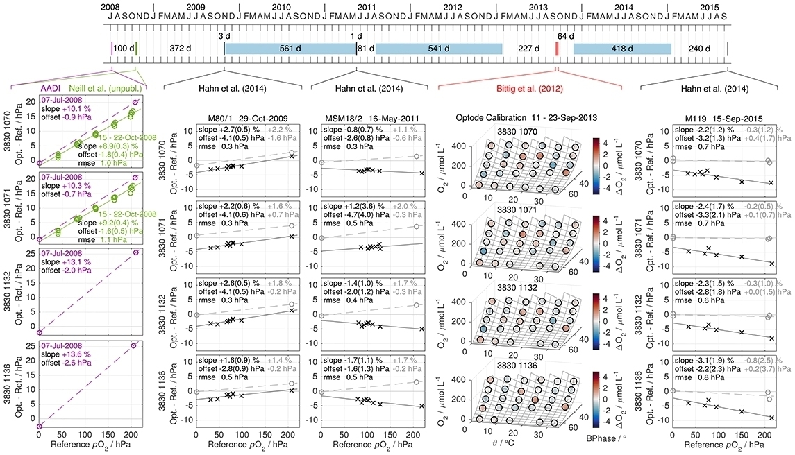
Figure 10. Laboratory calibration and in-situ reference data from four Aanderaa 3830 optodes used on moorings in the Eastern Tropical North Atlantic. The timing of factory batch two-point calibration (purple), BCCR Bergen and GEOMAR Kiel laboratory calibrations (green and red bar, respectively), on-ship calibrations (two-point laboratory and in-situ CTD casts, black bars), and moored periods (blue patches) along with the time difference between events (in days) is given on top. Below, residuals of the GEOMAR laboratory calibration (September 2013) are shown in (O₂, ϑ, φ)-space in the second column from right. The other four columns give the difference between laboratory-calibrated optodes and reference data against pO₂ in chronological order (2008, October 2009, May 2011, and September 2015). Laboratory data are denoted by circles and in-situ reference data by crosses. Optode and in-situ data are consistently offset by ca. −3 hPa for reasons unknown. Dashed lines denote linear two-point calibration fits while continuous lines give linear fits to multi-point data. In general, the optode O₂ drift character is well visible, with an exponentially decreasing O₂ sensitivity (linear with pO₂) and a zero offset that shifts toward more positive values. Apart from the offset, in-situ data suggest a significant drift during the first deployment period, while the on-ship two-point calibrations indicate stable optodes (second and third column). However, two-point data fit better to the laboratory calibration between second and third deployment than in-situ data. The evidence for drift or stability during deployment is thus mixed for these 4 optodes.

The general picture matches our O₂ optode understanding, with a very strong O₂ sensitivity reduction on the order of 10 % during the first years, and an exponential decrease of the drift rate. At the same time, the zero intercept shifts toward more positive pO₂ within each calibration approach. Moreover, the BCCR laboratory and the in-situ calibrations support a linear pO₂ drift dependence. However, all four optodes show a remarkably consistent offset at zero O₂ between laboratory calibrations and in-situ references of ca. −3 hPa for unknown reasons.

Regarding a potential drift during deployment, the first, 1.5 year-long deployment is best framed by on-ship and in-situ reference data, acquired just three days before deployment and one day after recovery. The other two deployment periods are less well constrained, as between 2 and 8 months passed between calibration and deployment or recovery, respectively. For these periods, we can not accurately assign an optode sensitivity drift to the period during deployment or during storage.

The on-ship two-point calibrations just before and after the first deployment agree with each other (mean difference of −0.1 % for the O₂ slope and of 0 hPa for the zero intercept), suggesting no drift during deployment. For the period between second and third on-ship two-point calibration, covering two more deployment periods (18 and 14 months) as well as 20 months of storage, optodes drifted toward lower O₂ sensitivity on average by 2 % over 4.3 years while the zero intercept increased by 0.5 hPa. This is a much smaller optode drift than initially during the first months and years (Figure 10), but in a reasonable range for O₂ sensitivity drift (e.g., during storage) of old optodes.

In turn, the in-situ reference data suggest a significant O₂ sensitivity change during the first deployment of −3 % (intercept increase by +1 hPa) over 1.5 years. For the second period, the O₂ sensitivity is reduced by 2 % on average and the intercept changes insignificantly (−0.2 hPa), which is comparable to the two-point data. However, while the two-point calibration data fit well with the multi-point laboratory calibration in September 2013, the in-situ reference data are somewhat below (including the −3 hPa offset). We can therefore draw no sound conclusion whether the moored optodes drifted during deployment from our mixed evidence. However, O₂-response drift may be an issue even during deployment, and we would recommend that adequate means are taken to track the temporal evolution of optode O₂ response in-situ.

4. Field Aspects

4.1. How to Calibrate O₂ Optodes

Oxygen optodes should receive an individual multi-point calibration at least once during their lifetime to have their O₂-T-response characterized well. The description of the O₂-T-response by a batch calibration of the sensing foil does not yield satisfactory results since variability between individual sensing foils and optodes is not adequately adjusted using a two-point calibration.

With a once well-characterized O₂-T-response, simpler means of recalibration can be appropriate when taking the optode drift character into account, i.e., a slope factor on optode pO₂ and an offset at zero oxygen. Data for such a recalibration can originate from various sources, e.g., a concurrent depth profile with discrete Winkler samples, optode in-air measurements at the surface together with hydrographic data on a deep isopycnal (to allow for a two-point correction), or a laboratory or on-ship calibration at 0 % and 100 % O₂ saturation (preferably in the temperature range at which the sensor will be deployed). In the latter case, care must be taken to avoid unintended supersaturation for the “100 %” calibration, in particular when using classical bubbling stones⁴. If only one cluster of reference data is available (e.g., only in-air measurements), preference should be given to a slope-only correction on pO₂.

4.2. What Accuracy Can Be Obtained

Numerous Aanderaa optodes have been deployed or used with only a factory batch calibration, in particular before the manufacturer introduced its factory multi-point calibration option in mid-2012. While it would be preferable to individually recalibrate each of these optodes, this is not always possible or practical, e.g., because the sensor is no longer accessible. To assess the quality of O₂ data obtained with such batch calibrated optodes, we compared calibration data from several multi-point laboratory calibrations with the batch calibration procedure. Similarly, (repeated) multi-point calibrations require some effort and may not be possible due to time, logistical or other constraints. We therefore looked at the accuracy of simpler recalibration approaches of multi-point calibrated optodes as well. Both assessments are summarized at the end of this section.

4.2.1. Refit Assessment

To assess the quality of the batch calibration approach, we derived the batch foil O₂-T-response ${{F}}_{\text{batch}}$ from the foil calibration certificate (using Equation 31). Subsequently, we adjusted or refit ${{F}}_{\text{batch}}$ for each optode multi-point calibration by (1) varying the amount of information provided to the refit and (2) varying the kind of refit. In fact, both the choice of reference points (1) and the choice of refit Equation (2) are critical.

For (1) the choice of reference points, we tested three approaches of increasing information but also increasing operational demand: (i) two points close to the Aanderaa two-point calibration standards, (ii) 4 references at 0 % and 4 references near 100 % O₂ saturation, each stretched between 4 °C and 36 °C, and (iii) all reference points available from the full multi-point calibration matrix (20–45 points). Case (iii) basically assesses how well ${{F}}_{\text{batch}}$ can be mapped to the individual optode response with the given refit approach (2), while (ii) and (i) give an estimate of this mapping with limited information.

For (2) the choice of refit equation, we systematically tested all kinds of refits with two degrees of freedom with a slope and/or offset on temperature, phase, or oxygen (not shown). Similarly, we proceeded with refits using three degrees of freedom (only slope and/or offsets, no squared terms).

The quality of the refit was quantified with the 90-th percentile of the absolute pO₂ difference between adjusted-batch calculation and individual multi-point calibration-based calculation (using again Equation 31), i.e., 90 % of the data were within the given ΔpO₂ for the individual refit. To adequately cover the variability within the sensing foil batch and differences between sensors, we averaged the results from multiple recalibrations (and thus refits) of the same sensor—sensing foil pair. This avoids a bias of optodes calibrated several times over optodes calibrated only a few times within a given foil batch, and increases the robustness of the individual sensor—sensing foil refit estimate. Finally, the quality of the sensor—sensing foil pair refits was quantified by the 90-th percentile on the foil batch level (Table 1), i.e., for 90 % of the optodes of a foil batch we encountered, 90 % of the data were within the given ΔpO₂ for the respective refit approach.

TABLE 1

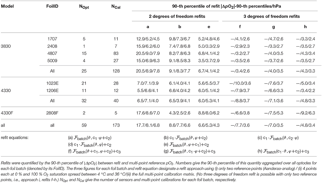
Table 1. Accuracy of batch foil O₂-ϑ-response adjustment to individual multi-point optode calibrations using refit approaches with two (a–e) and three degrees of freedom (f–h).

To assess the quality of adjustments for multi-point calibrated optodes, we followed the same approach as above, except that we used only optodes that have been calibrated several times (27 Aanderaa optodes with 152 calibrations and 4 Sea-Bird optode with 12 calibrations). For each optode, one multi-point calibration was used to derive individual calibration coefficients ${{F}}_{\text{multi}}$ (using Equation 31). Subsequently, the other multi-point calibrations were used to adjust or refit ${{F}}_{\text{multi}}$ by (1) varying the amount of information provided to the refit and (2) varying the kind of refit as above. This procedure was repeated for all calibrations of a given optode to avoid a bias by the choice of the initial calibration to derive ${{F}}_{\text{multi}}$. Again, the 90-th percentile of the absolute pO₂ difference between adjusted (initial) multi-point calculation and multi-point recalibration-based calculation served to quantify the quality of the refit. The results were averaged over all ${{F}}_{\text{multi}}$'s for a given optode multi-point calibration, and then averaged for each optode (i.e., on the sensor–sensing foil pair level) to avoid a dominance of sensors with many recalibrations over sensors with only a few. No differences between foil batches were discernable. Table 2 thus gives the 90-th percentiles of the |ΔpO₂|-90-th percentiles aggregated on the sensor model level as well as for all sensors.

TABLE 2

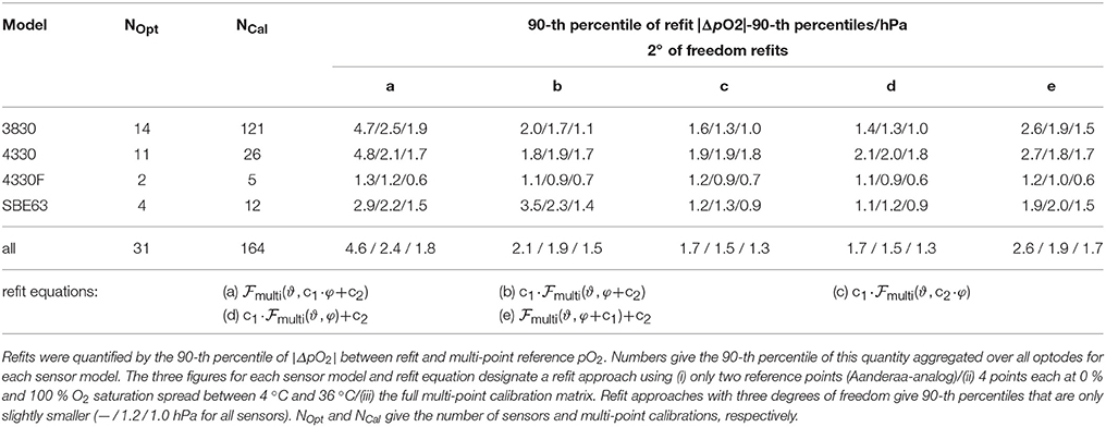
Table 2. Accuracy of multi-point ${{F}}_{\text{multi}}$ O₂-ϑ-response adjustments to individual multi-point optode calibrations using refit approaches with two degrees of freedom (a–e).

4.2.1.1. Batch-calibrated optodes

The factory batch calibration procedure of Aanderaa optodes consists of two steps, (1) a multi-point characterization of the O₂-T-response for 4 out of 100 sensing foils of a given batch, and (2) adjustment of this batch response (in phase- or O₂-space, depending on calibration date) to the individual sensor by a two-point calibration (at 100 % O₂ saturation and 10 °C, and at 0 % O₂ saturation and 20 °C). The adjustment or refit is supposed to compensate several effects:

• variability within the sensing foil batch

• a sensing foil O₂ response drift that may have occurred between batch and two-point calibration

• differences between the reference and sensor phase measurements

In that respect, the batch calibration adjustment or refit is conceptually different from an O₂ response drift correction, which exclusively aims at the O₂ response drift (see below). An example of the refits given in Table 1 for a model 3830, 4330, and 4330F batch-calibrated optode is shown in Figure S9.

Using approach iii, i.e., data of the full O₂-T calibration matrix, we assessed the suitability of all refits to reproduce the multi-point calibrations to select appropriate refit equations (not shown). With 2 degrees of freedom, the highest accuracies for foil batch refits were obtained with refit e, refit b, and refit a, followed by refits c and d (in this order; refit equations are given at the bottom of Table 1). If only limited information is available for the refit (approach ii), refits c and d slightly outperform refit a (not shown). With three degrees of freedom, refits f–h are best suited (refit equations given at the bottom of Table 1).

Refit equation a corresponds to the traditional, phase-domain adjustment used by Aanderaa and also proposed by Drucker and Riser (2016) (slope and offset on φ). It gives the highest uncertainty (up to 18 hPa for all optodes for a two-point adjustment; approach i), mainly due to issues in a proper temperature compensation of ${{F}}_{\text{batch}}$ (e.g., Figure S9a). Refits b–d share a slope factor on pO₂ (together with a phase offset, a slope on phase, or a pO₂ offset, respectively) and should thus be primed to account for an O₂ sensitivity drift (see section 3.5.1.1). Out of this group, refit b with an offset on φ performs best. The most accurate results for a two degrees of freedom equation, however, are obtained with refit e, which combines an offset on both φ and pO₂. Also note that the best refits with three degrees of freedom (refits f–h) are based on refit e. An offset on the sensor's phase shift φ thus seems to be of prime importance to adjust a batch foil calibration ${{F}}_{\text{batch}}$ to the individual sensor, most likely to account for differences between the reference and sensor phase measurements.

When using not only one reference point at 0 and 100 % O₂ saturation (approach i), but a set of 0 and 100 % O₂ saturations at a wide temperature range (approach ii), the uncertainty of the refit can be significantly reduced (range of 1–10 hPa for the given refit equations). However, this expansion of the temperature range affects mostly refit a (improvement of 10 hPa), whereas the other refits benefit to a smaller degree (1–3 hPa), but nonetheless become more robust (through using more reference points). This underlines that a phase-domain adjustment does not adequately capture and correct the O₂-T-response. Compared to using the full calibration matrix (approach iii), approach ii tends to be 1–3 hPa less accurate for refits with two degrees of freedom, and 1–5 hPa less accurate for the refits with three degrees of freedom.

Adding a third degree of freedom generally improves the refit (by ca. 1 hPa) when using all data (approach iii). However, adding another degree of freedom in multidimensional space while using reference data that does not cover all dimensions can yield adverse results. With limited information (approach ii), refits f–h tend to perform only as good or even worse as refit e. Here, reference data covers well the temperature dimension (2 × 4 samples) but is poorly resolved in the oxygen dimension (4 × 2 samples only at 0 % and 100 % O₂ saturation). Consequently, the extra degree of freedom can be used to reduce the mismatch along ϑ while sacrificing accuracy at intermediate and supersaturated O₂ levels (e.g., refit e vs. refit f/g, Figure S9b). In case of reference approach ii, we would therefore recommend to keep refit equation e with only two degrees of freedom.

For the two 4330 optode foil batches that we encountered, the traditional two-point adjustment approach i together with refit a performs much better (7 hPa) than for the other foil batches. One could speculate that the temperature dependence of 4330 foil batches is already well-described by ${{F}}_{\text{batch}}$ compared to 3830 foil batches, since their batch calibration uses 9 temperatures between 3 and 40 °C instead of 5. However, this would hold for the fast response foil batch 2808F, too, where we observe the same pattern as for 3830 foil batches for refit a. Moreover, differences between refits b–e are small for the 4330 optode foil batches. In fact, refit b gives the lowest uncertainty both for 4330 and 4330F optodes when combined with recalibration approach ii, i.e., limited information in both O₂ and ϑ. Their refit uncertainty is comparable to approach iii.

Our results thus suggest to use refit e with recalibration approach i (i.e., two-point calibration), refit e with approach ii for 3830 optodes and refit b for 4330 optodes, and to derive a complete multi-point calibration ${{F}}_{\text{multi}}$ of its own with approach iii (i.e., full calibration matrix). Approach iii here only gives the lower accuracy limit of the respective refit equations (Table 1).

4.2.1.2. Multi-point calibrated optodes

A multi-point calibration characterizes the O₂-T-response for each individual sensing foil–sensor pair. A later adjustment or refit is thus only supposed to compensate one effect:

• a sensing foil O₂ response drift that may have occurred between multi-point and re-calibration.

For multi-point calibration refits with two degrees of freedom, refit Equations b–d give the best, hardly distinguishable results (Table 2). Refits a and e were added for comparison. The results underline that O₂ sensitivity drift should be corrected with a factor on O₂ (also compare refit a vs. refits b–d, Table 2).

For refits with three degrees of freedom, 5–7 out of the 20 possible refit equations are near-indistinguishable (not shown), and the improvement for multi-point calibrations adjustments is only marginal compared to refits with two degrees of freedom (90-th percentiles of — / 1.2 / 1.0 hPa for the three approaches i / ii / iii vs. 1.7 / 1.5 / 1.3 hPa using refits c and d). We therefore recommend to refit multi-point calibrations with two degrees of freedom and to invest the effort of additional reference points (i.e., approach ii vs. approach i) into better constraining the two parameters rather than adding a third degree of freedom. From our analysis, a slope correction on pO₂ together with either a slope on φ or an offset on pO₂ (refits c and d) give an adjustment closest to the multi-point calibration data (1.7 hPa for a two-point calibration; approach i).

4.2.2. Summary and Decision Tree/Flow Chart

The accuracy of an optode calibration is the sum of three factors: (1) The quality of the O₂-T-response characterization, (2) the refit accuracy, and (3) the O₂ sensitivity drift, both when not deployed (section 3.5.1) and when deployed (section 3.5.2).

For the GEOMAR Kiel and the BCCR Bergen / CSIRO-O&A Hobart calibration setups, we looked at all multi-point calibrations against Winkler samples and determined the 90-th percentiles of the absolute pO₂ calibration residuals (using Equation 31). The 90-th percentile of all calibrations is 1.5 and 0.9 hPa, respectively, which we take as representative for the quality of multi-point calibrations (1). We assume that the batch foil characterization occurs with a comparable accuracy against reference samples. The refit accuracy (2) has been discussed above, where the numbers give the difference between refit (with only a subset of the multi-point data) against a multi-point calibration (using all multi-point data), i.e., the “excess” uncertainty introduced by the refit. For the O₂ sensitivity drift, we take a conservative estimate of 5 % per year (10 hPa per year) for “storage” drift and 0.5 % per year (1 hPa per year) for drift in-situ. The storage drift magnitude is probably lower for old sensing foils, but not uncommon for new sensors (e.g., D'Asaro and McNeil, 2013; this work, Figure 7). The accuracy that can be obtained with O₂ optodes depends thus on a range of factors, how the sensor was prepared, and how it is deployed, which is summarized as a flow scheme in Figure 11. It covers an order of magnitude from 1 hPa (i.e., meeting the accuracy goal of Gruber et al., 2010) for sensor deployments that were carefully prepared to more than 20 hPa for optodes just used out of the box.

FIGURE 11

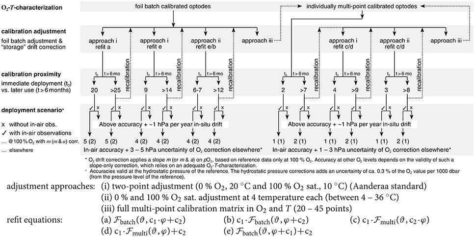
Figure 11. Scheme to estimate the accuracy (in hPa) achievable with Aanderaa and Sea-Bird oxygen optodes. The accuracy depends (1) on the kind of O₂-T-response characterization (batch vs. multi-point), (2) the kind of adjustment/refit to the individual sensor, (3a) its temporal proximity to the deployment (e.g., drift during storage or shipment), as well as (3b) whether in-air observations are performed during the deployment. With in-air observations, the accuracy at 100 % O₂ saturation is given once using (Equation 21) (to derive a correction factor m) and once using (Equation 23) (to derive a correction factor m by including a temperature-compensation a of the O₂-T-response at 100 %; in brackets). At O₂ levels other than 100 % O₂ saturation, some additional uncertainty remains with respect to the in-situ drift behavior and the O₂-T-response. The hydrostatic pressure correction adds an uncertainty of ca. 0.3 % of the O₂ value per 1,000 dbar (from the pressure level of the reference / calibration). The adjustment approaches i–iii and refit equations a–e are given at the bottom of the scheme.

We propose to do the accuracy estimate in pO₂ (see Figure 11), since that is what the optode is sensitive to, and then convert it to the desired unit. For water column applications, a pressure correction uncertainty of 0.3 % of the pO₂ should be added per 1000 dbar (Bittig et al., 2015a), starting from the depth(s) of the reference(s), i.e., from the surface for laboratory calibrations or when the optode was in-situ adjusted with in-air observations, or from 2000 dbar if the sensor was in-situ adjusted by comparison with reference data at 2,000 dbar depth.

4.3. How to Deal with O₂ Response Drift

4.3.1. During Storage: Timely Reference or (Re-)Calibration

The aim for every optode deployment should be to acquire sufficient information shortly before deployment or after recovery to enable a proper drift correction, i.e., to provide data with at least two (clusters of) reference points. Reference data can originate from any source (e.g., from a concurrent and ideally co-located Winkler-based CTD-O₂ profile at deployment, hydrographic databases, in-situ in-air measurements, etc.) since the kind of correction is independent of how the reference data were obtained. Even better but more demanding would be a timely, full multi-point recalibration of the optode to cover the entire O₂-T-response and to avoid having to use assumptions on the drift character. If it is impossible to obtain any in-situ data (e.g., when deploying from a ship of opportunity), the main optode drift (the O₂ sensitivity drift) can be roughly assessed through on-deck in-air measurement of the optode before deployment under controlled conditions (i.e., sun-shaded, windward-side with proper barometric pressure data).

4.3.2. During Deployment: In-Air Measurements

There might be chance-encounters or deliberate crossovers with other oxygen observations during the deployment of an oxygen optode. Given the limitations due to either the proximity or the accuracy of other platforms' oxygen observations, it is preferable to achieve regular reference measurements with the optode itself. For profiling applications, this is feasible through regular optode in-air measurements which are recommended by the SCOR Working Group 142 (Bittig et al., 2015b) and have been implemented on profiling floats and gliders. They should become a requirement for autonomous oxygen observations to ensure O₂ data quality. Major float manufacturers have already started to implement this function into their float routines.

For properly utilizing such data, one needs to take into account that optode measurements “in air” close to the sea surface do not measure pure air but an air-water mixture. Therefore, such measurements must be corrected for a “carry-over” effect (Equation 18). Accuracy can be easily improved by making multiple measurements in air during each surfacing (e.g., Bittig and Körtzinger, 2015; Bushinsky et al., 2016). Moreover, data suggest that preference should be given to nighttime in air observations, which will not always be possible though, e.g., on a Biogeochemical-Argo float with concurrent radiometric measurements.

For moored applications, regular reference measurements, e.g., through in-air observations have only been described for surface moorings (Bushinsky and Emerson, 2013) and are likely impossible elsewhere. In such cases, on-deck in-air measurements or on-ship calibrations immediately prior to deployment and after recovery (see, e.g., section 3.5.2.2) are a promising approach to frame the O₂ response evolution during deployment.

4.4. How to Improve the Dynamic Time Response

The key and core requirement to correct for the dynamic time response of optodes is to know the time interval between subsequent measurements (or to have at least a good estimate of the timing of each sample). Without timing information, no post-correction is possible since the dynamic time response is essentially a time series effect. To date, the Biogeochemical-Argo data system is capable to store abundant measurement timing information together with the profile data (Bittig et al., 2017). Previously, this has not been the case and the acquisition and storage of timing information has been the responsibility of the platform operator.

The key to reduce the effect of the dynamic time response itself is to enhance the flow and thus the transfer of O₂ at the interface between sensing foil and sea water. To achieve this, optodes can either be operated in a pumped water stream if feasible with respect to the energy budget and additional constraints like in air measurement capability. Or, in an unpumped mode of operation, optodes should be placed at a position on the platform with the most dynamic flow regime and hence thinnest boundary layer (compare, e.g., optode placement on a glider for Nicholson and Feen, 2017, with the standard attachment shown in Bittig et al., 2014). In any case, a reproducible and properly characterized flow regime helps to improve time response corrections (e.g., Bittig and Körtzinger, 2017).

4.5. How to Ensure a Successful Deployment: Preparation, Preparation, Preparation

A successful deployment comes with adequate preparation. The sensor configuration should always be kept for reference, and the treatment of the data stream anticipated before deployment (e.g., to adjust the platform's firmware to actually log and transmit timestamps for each optode sample). Raw data should be kept to allow reprocessing and to keep all information provided by the sensor. Apart from the measurement time, these data are the temperature and phase delay for Sea-Bird SBE63 optodes, whereas the temperature and the blue phase shift (BPhase or C1Phase for 3830 and 4330 models, respectively) as well as the red phase shift (C2Phase for 4330 models) should be kept for Aanderaa optodes.

Moreover, O₂ optodes should always be assumed to be out of calibration if not very recently calibrated (weeks for newly produced optodes, months for old ones). Consequently, options for reference O₂ data (e.g., by regular in-air measurement or other approaches) need to be explored before deployment.

5. Data Processing

5.1. What O₂ Unit Should I use?

Dissolved oxygen comes in various units, e.g., μmol O₂ kg⁻¹, μmol O₂ L⁻¹, mL_STP O₂ L⁻¹, mg O₂ L⁻¹, hPa, or % O₂ saturation, which at the end of the day all carry the same information (i.e., the amount of dissolved oxygen). This indeed is a confusing aspect of dealing with oceanic O₂ measurements and the general practice should be to always double-check the unit of a new data set, e.g., by verifying that surface O₂ saturation is within a reasonable range. However, each unit has its strength by stressing a different aspect of oxygen measurements and analysis, and it is best to be aware of the reasons for this (persistent) plurality.

Oxygen concentration can be expressed in two ways, either as number of moles of dissolved oxygen per unit mass of solution (μmol O₂ kg⁻¹; gravimetric unit) or per unit volume of solution (μmol O₂ L⁻¹, mL_STP O₂ L⁻¹, mg O₂ L⁻¹; volumetric unit). The unit μmol O₂ kg⁻¹ is the unit of choice for oceanic applications because of its independence of temperature and pressure, both of which will change the concentration when expressed in a volumetric unit even without any production or consumption of oxygen. To allow using of O₂ as a conservative tracer for ocean mixing and advection, μmol O₂ kg⁻¹ is the recommended unit for oceanic applications and used by all larger observing systems (see, e.g., documentation for GO-SHIP and Biogeochemical-Argo, Hood et al., 2010, and Thierry et al., 2016).

The standard reference method for O₂ is a wet-chemical titration analysis (e.g., Winkler, 1888; Carpenter, 1965) which essentially is a volumetric analysis, i.e., it yields the amount of O₂ in a given sample volume. Thus, the natural unit for Winkler titration is μmol O₂ L⁻¹. This holds for laboratory applications in general, and seagoing applications in particular, where measuring volumes of solutions is much more common than measuring their mass, which is impossible at sea. Moreover, O₂ concentration units per volume (e.g., mL_STP O₂ L⁻¹, mg O₂ L⁻¹) are also common for limnological applications.

Gravimetric and volumetric oxygen concentration can be converted by multiplying/dividing with the solution's density (mass per volume). For seawater, this gives about 3 % larger values for the O₂ concentration in μmol L⁻¹ than in μmol kg⁻¹, a difference that is difficult to spot but very important for applications. Therefore, care must be taken when dealing with a new data set and it is best practice to verify the O₂ unit, e.g., by confirming reasonable surface O₂ saturations or deep O₂ levels.

At interfaces like the sea surface or the optode sensing foil—water interface, oxygen data solely expressed as water-based O₂ concentration are not sensible, in particular when part of the observations are in different phases. At interfaces, the oxygen partial pressure pO₂ and a corresponding pressure unit (e.g., hPa) is the natural quantity and unit for both phases. We would discourage the use of atmospheres (atm, 101,325 Pa) but suggest to use a full power of ten of the SI unit Pascal (e.g., hPa, bar, or mbar).

Detailed conversions between the units listed here are given in the SCOR Working Group 142's recommendations on O₂ quantity conversions (Bittig et al., 2016). Converted values for 100 % O₂ saturation, 205 hPa, and 250 μmol L⁻¹ both in freshwater and at a salinity of 35 as well as at the surface and at 2,000 dbar are shown in Table S4.

5.2. How to Calculate O₂

5.2.1. Data Validation

The first step of optode O₂ calculations is to check the raw data (optode temperature ϑ, optode phase shift φ) and ancillary data (e.g., salinity S, hydrostatic pressure P, …) for completeness and consistency with any other concurrent observations (e.g., CTD temperature), for an adequate range (compare, e.g., with the valid ranges defined for Biogeochemical-Argo: Schmechtig et al., 2016, and “Argo physical parameters list: Core-Argo and BGC-Argo” at http://www.argodatamgt.org/Documentation⁵), and whether they are sensible.

5.2.2. O₂ and Temperature Compensation

Next, all environmental factors that affect the O₂ measurement need to be accounted for (section 3). There are various ways described in the literature to account for the O₂-T-response, i.e., the mapping ${F}(T,\phi )\to {\text{O}}_2$ (Equation 12):

The standard way for Sea-Bird SBE63 optodes to calculate a (freshwater-equivalent) O₂ concentration follows a modified version of Uchida et al. (2008),

$\begin{array}{ll}{c_{{\text{O}}_2,\text{adj}}|}_{S=0}=\frac{\frac{{\text{c}}_4+{\text{c}}_5·\vartheta +{\text{c}}_6·{\phi }_{\text{adj}}^2}{{\text{c}}_7+{\text{c}}_8·{\phi }_{\text{adj}}}-1}{{\text{c}}_1+{\text{c}}_2·\vartheta +{\text{c}}_3·{\vartheta }^2},& (24)\end{array}$

where φ_adj is the optode's adjusted phase delay in μs (see Equation 28, section 5.2.4 below), ϑ the optode temperature in °C, and c_1…8 the eight calibration coefficients (Sea-Bird Electronics, 2013). The standard unit for the SBE63 optode factory calibration is mL_STP O₂ L⁻¹.

For Aanderaa optodes, the mapping ${F}(T,\phi )$ evolved significantly with time (an exhaustive description of different cases can be found in Thierry et al., 2016). Previously, only “batch-calibrated” optodes were available. Here, 4 out of a batch of 100 sensing foils are calibrated in detail with respect to their non-linear O₂-T-response and their behavior is assumed to be representative for the entire batch. The non-linear behavior is described by so called foil coefficients that parameterize a high-order polynomial with 20 terms up to order 4 in phase and order 3 in temperature for 3830 optodes (${{F}}_{3830}$, see Aanderaa Data Instruments AS, 2006) and with 27 terms (of which typically only 21 are non-zero) up to order 5 in both phase and temperature for 4330 optodes (${{F}}_{4330}$, see Aanderaa Data Instruments AS, 2009). Subsequently, each individual sensor—sensing foil pair is two-point calibrated with one point at zero O₂ and room temperature and one point at 100 % O₂ saturation near 10 °C. Depending on the version of the calibration certificate, these data were used for a linear (offset and slope) correction either on the phase shift (“phase-domain”), on the result of ${F}$ (“oxygen-domain”) or at both locations, i.e.,

$\begin{array}{ll}{c_{{\text{O}}_2,\text{adj}}|}_{S=0}={\text{c}}_1·{{F}}_{3830/4330}(\vartheta ,{\text{c}}_3·{\phi }_{\text{adj}}+{\text{c}}_4)+{\text{c}}_2& (25)\end{array}$

where φ_adj is the optode's adjusted phase shift in ° (see Equation 28, section 5.2.4 below), ϑ the optode temperature in °C, and ${{F}}_{3830}$ and ${{F}}_{4330}$ the polynomial function of foil coefficients for 3830 or 4330 optodes, respectively. c_1/2 are the so called ConcCoefs and c_3/4 the first two PhaseCoefs (Aanderaa Data Instruments AS, 2009). Since mid-2012, Aanderaa optode models 4330 can be individually multi-point calibrated by the manufacturer. The calibration data are used to derive seven calibration coefficients c_1…7 following Uchida et al. (2008) to calculate a (freshwater-equivalent) O₂ concentration,

$\begin{array}{ll}{c_{{\text{O}}_2,\text{adj}}|}_{S=0}=\frac{\frac{{\text{c}}_4+{\text{c}}_5·\vartheta }{{\text{c}}_6+{\text{c}}_7·{\phi }_{\text{adj}}}-1}{{\text{c}}_1+{\text{c}}_2·\vartheta +{\text{c}}_3·{\vartheta }^2}.& (26)\end{array}$

All Aanderaa factory calibrations provide O₂ in units of μmol O₂ L⁻¹.

As discussed for the in-air measurements, the two-point calibration of batch foil coefficients is inadequate to fully adjust the O₂-T-response to each individual optode. Therefore, an individual multi-point calibration for every optode is advisable to allow high-quality O₂ data.

In addition, the above Uchida et al. (2008)-type mathematical model ${F}$ (Equation 26) has the advantage of a better interpolation and in particular extrapolation behavior with respect to the scattered calibration data compared to the high-order polynomial mathematical models ${{F}}_{3830}$ and ${{F}}_{4330}$ (Equation 25). However, the mathematical model ${F}$ is always independent of the calibration or reference data itself. Matlab code to refit calibration coefficients after Equations (26, 31) from Aanderaa batch calibration data sheets is provided by Bittig (2018).

5.2.3. Salinity Compensation

The response of oxygen optodes is sensitive to the partial pressure pO₂ of the ambient medium. For mathematical models ${F}$ that do not provide the pO₂ directly but a (freshwater-equivalent) O₂ concentration in the ambient medium (i.e., all the ones mentioned in section 5.2.2), the result of ${F}$ needs to be corrected for the salinity dependence of the conversion between O₂ concentration and partial pressure, i.e.,

$\begin{array}{ll}{c_{{\text{O}}_2,\text{adj}}|}_S=\frac{1013.25\text{ hPa }-p{\text{H}}_2\text{O}(\vartheta ,S=0)}{1013.25\text{ hPa}-p{\text{H}}_2\text{O}(\vartheta ,S)}·{\text{S}}_{\text{Corr}}·{c_{{\text{O}}_2,\text{adj}}|}_{S=0},& (27)\end{array}$

where pH₂O is the partial pressure of water vapor (Weiss and Price, 1980) and S_Corr the salinity-dependent factor of the O₂ solubility $c_{{\text{O}}_2}^{*}$ following Garcia and Gordon (1992) using the Benson and Krause refit (see Bittig et al., 2016). Note that the salinity corrections given by both Aanderaa and Sea-Bird are not fully correct since they neglect the salinity-dependence of pH₂O and thus the associated (albeit small) change in atmospheric equilibrium pO₂ (Bittig et al., 2016).

5.2.4. Hydrostatic Pressure Compensation

The pressure correction of optode observations should be done in two steps to account for the two different processes observed in laboratory studies (Bittig et al., 2015a). To compensate the pressure effect on the luminescence lifetime Λ₀, the raw phase measurement φ_raw from the optode should be adjusted following Equation 28 with a phase offset z depending on the sensing foil and manufacturer (PSt3 foils: 0.100° per 1,000 dbar for Aanderaa optodes, 0.115 μs per 1,000 dbar for Sea-Bird optodes).

$\begin{array}{ll}{\phi }_{\text{adj}}={\phi }_{\text{raw}}+z·P& (28)\end{array}$

After application of the oxygen, temperature, and salinity compensation to the adjusted phase data φ_adj (subsections 5.2.2 and 5.2.3), the pressure effect on quenching and on the membrane O₂ equilibrium level can be corrected by

$\begin{array}{ll}{c}_{{\text{O}}_2}=c_{{\text{O}}_2,\text{adj}}·\left(1+f(\vartheta )·P\right)& (29)\end{array}$

with f(ϑ) following

$\begin{array}{ll}f(\vartheta )/\%\text{ per }1,000\text{ bar }=4.19+0.022·\vartheta & (30)\end{array}$

for both Aanderaa optodes and Sea-Bird optodes. The uncertainty in f is ca. 0.3 % per 1000 dbar (Bittig et al., 2015a), i.e., wherever the reference data are obtained (e.g., in the laboratory or near the surface from in-air measurement vs. at depth from hydrographic data), the uncertainty of the optode measurements increases by this amount the farther they are from the pressure level of the reference data.

5.2.5. Simplification of Optode Calculations

The above steps can be simplified into one by using a mathematical model ${F}$ that provides the partial pressure pO₂ instead of an estimate of the O₂ concentration that depends on conditions (either a freshwater setting with S = 0 or a subsequent salinity-correction to give sensible results). The advantage of pO₂ mathematical models is that (1) they avoid the ambiguity of c_O2,adj|_S=0 vs. c_{O2, adj}|_S which by necessity have the same unit and are thus easily confused, (2) they provide a sensible O₂ quantity directly (see section 5.1), and (3) they adequately represent the processes at work, i.e., the interface and equilibrium between optode sensing foil and ambient seawater medium.

At GEOMAR, good experience has been obtained with a modification of Uchida et al. (2010) following

$\begin{array}{ll}p{\text{O}}_{2,\text{adj}}=\frac{\frac{1+{\text{c}}_4·\vartheta }{{\text{c}}_5+{\text{c}}_6·{\phi }_{\text{adj}}+{\text{c}}_7·{\phi }_{\text{adj}}^2}-1}{{\text{c}}_1+{\text{c}}_2·\vartheta +{\text{c}}_3·{\vartheta }^2}.& (31)\end{array}$

that in general yields lower root-mean-squared-errors to calibration data than the original Uchida et al. (2008) model (Equation 26), its Sea-Bird modification (Equation 24), or the McNeil and D'Asaro (2014) model. Again, the kind of mathematical model ${F}$ is independent of how calibration data were obtained and any kind of mathematical model can be applied to calibration data of arbitrary origin. Matlab code to refit Aanderaa batch calibration data (as well as Aanderaa and Sea-Bird multi-point factory calibrations for comparison) according to Equation (31) is provided by Bittig (2018).

Comparison of Equations (14, 15, and 29) gives

$\begin{array}{ll}p{\text{O}}_2=p{\text{O}}_{2,\text{adj}}·\left(1+f(\vartheta )·P\right)·\exp \left(\frac{{\text{V}}_{\text{m}}^L({\text{O}}_2)·P}{\text{R }·(\vartheta +273.15\text{ K})}\right)& (32)\end{array}$

to correct pO_2,adj from Equation (31) for the effects of hydrostatic pressure.

For surface applications, Equation 31 gives a fully valid O₂ quantity in one step. With hydrostatic pressure effects, Equations (28, 31, and 32) (including Equation 30) need to be combined. Conversions from pO₂ to O₂ concentration or other O₂ quantities are easily done using the SCOR Working Group 142's recommendations on O₂ quantity conversions (Bittig et al., 2016).

5.2.6. Dynamic Time Response Correction

Time response correction is basically inverse filtering or deconvolution of the optode observations to remove the smoothing and lag of the optode time response. This, however, includes all caveats that come with this operation, in particular amplification of noise in the observations, which can create artifacts especially in regions of strong and/or changing O₂ gradients. To permit an accurate reconstruction, data need to be logged at an adequate temporal resolution (with respect to the magnitude of τ) and the response time estimate should be appropriate. One possible algorithm is described in Miloshevich et al. (2004), which has been applied by Fiedler et al. (2013) to oceanic pCO₂ observations. The algorithm given in Bittig et al. (2014), which they also used to correct O₂ optode data, is reproduced in the Supplemental Material.

Unrealistic overshoots (e.g., at the base of the mixed layer) or similar artifacts in changing O₂ gradients can occur, e.g., due to a too coarse temporal resolution of the data or an inadequate response time τ estimate. In such cases, the magnitude of the correction should be manually reduced, e.g., by lowering τ's by 10 %.

6. Summary

Driven by the growing interest in the marine oxygen cycle and motivated by the prospects of a global Biogeochemical Argo program (http://biogeochemical-argo.org), the oceanographic community has invested a great deal of effort into characterizing and understanding the promising oxygen optode technology. Through thorough laboratory and field studies on the one hand and careful analyses and theoretical considerations of the data on the other hand, a consistent picture of the properties, limitations and best practices has emerged for the most prominent commercially available oceanographic optode-based oxygen sensors. We have tried to put this here together in a comprehensive but still concise way. The main findings (following the structure of the manuscript) can be summarized as follows:

• Oxygen optodes are based on the principle of dynamic luminescence quenching the theory of which is well understood. All oxygen optodes show a non-linear Stern-Volmer behavior.

• Mathematical models to describe the sensor O₂-T-response do not adequately follow physical relationships⁶, however, they are able to properly describe the sensor response for practical purposes. Preference should be given to mathematical models with a small number of calibration coefficients, i.e., without high-order polynomials.

• Oxygen optodes respond to the partial pressure of O₂ (pO₂), which is independent of salinity. For a conversion to O₂ concentration both in volumetric (μmol L⁻¹) and gravimetric units (μmol kg⁻¹), the salinity-dependence of the conversion between pO₂ and O₂ concentration has to be taken into account by means of a “salinity correction”.

• Pressure affects the O₂ measurement in two ways, destabilizing the luminophore as well as reducing the amount of quenching, which requires a two-fold compensation for application at greater depths.

• The optode response to a change in ambient O₂ concentration is not instantaneous. This has consequences for profiling applications. Operation of optodes in pumped mode is characterized by significantly shorter response times. Response times in unpumped operations depend on the platform-dependent flow regime in front of the sensing window. Lookup tables allow estimation of response time as a function of T and flow regime for optodes with PSt3 sensing foils (Aanderaa and Sea-Bird optodes).

• Optodes with PSt3 foils generally show significant drift (i.e., several percent per year) when not submerged continuously in seawater, i.e., during storage and transport. Drift is linear with oxygen and can be corrected by a corresponding slope factor and zero offset. The slope correction should be applied on oxygen, not phase, and works best with pO₂. The drift is strongest in new optodes (foils) and less in older ones.

• This means that optodes with PSt3 foil should be regarded as uncalibrated unless they have been calibrated very recently, i.e., within a couple of weeks for new optodes, few months for optodes older than 5 years.

• Optodes are far more stable when deployed in the ocean. The majority of optodes with PSt3 foil are characterized by a moderate (mostly negative) drift, which typically does not exceed 0.5 % year⁻¹. This may be tolerable for shorter deployment but can accumulate to several percent over multi-year deployment such as on Argo floats.

• Since PSt3 sensing foils become more stable with time, we recommend to not replace them unless they are mechanically damaged. We have not experienced a limit for the lifetime of sensing foils due to aging factors other than mechanical damage.

• Depending on the kind of optode calibration, handling and usage scenario, accuracy of O₂ measurements can vary considerably (from 1 hPa to more than 20 hPa, see Figure 11 for PSt3 foil optodes). To achieve highest accuracy, each sensor requires an individual multi-point calibration in T- and O₂-space at least once during its lifetime. Foil batch calibrations fail to achieve such high accuracy.

• To correct for any possible drift prior to and after deployment as well as any in-situ drift (which on a few optodes may significantly exceed the typical 0.5 % year⁻¹ drift rate) some means of in-situ calibration should be implemented. When optodes can be recovered after deployment, an in-situ calibration at deployment and recovery is recommended. For deployments where the optode regularly gets in contact with air (e.g., on floats and gliders), the well-established in-air measurements routine can be implemented. This should be done by default for float-mounted optodes for which detection of in-situ drift is not straightforward otherwise. A minimum standard calibration routine should involve a two-point calibration (at 0 and 100 % oxygen saturation) at deployment and—for glider, moorings etc.—at recovery. During the lifetime of an optode-foil combination, drift effects can be compensated with, e.g., simpler two-point calibrations, if their O₂-T-response has been well characterized once by an individual multi-point calibration.

• The “smearing” effect of the response time on O₂ measurements can be corrected for if data are logged at adequate temporal resolution and with precise time stamps. Time response correction is basically inverse filtering the optode data, with all caveats that come with it (e.g., amplification of noise). Nonetheless, we found that it improves data quality. However, the response time effect on O₂ accuracy depends strongly on response time (i.e., flow) and O₂ gradient, ranging from near negligible to several tens of μmol kg⁻¹.

• No single O₂ quantity is suitable to express all aspects of O₂ observations, e.g., (dis-)equilibrium between air and water or water and sensing foil (O₂ saturation or pO₂), or water mass mixing (O₂ concentration). They give, however, the same information and we recommend to follow the SCOR WG 142 recommendations for conversions (Bittig et al., 2016). For sea water concentration, μmol kg⁻¹ should be the preferred unit. For partial pressure, we advise to use hPa or another full power of 10 of the SI unit rather than atmospheres (atm).

Aanderaa O₂ optodes (and to some degree Sea-Bird optodes) with PSt3 foils are by far the most well-studied. Following the guidance of this manuscript, they can be prepared to provide O₂ data with an accuracy of 1 hPa. Knowledge and experience with other O₂ optodes (JFE Advantech, Contros, RBR, Aanderaa optodes with WTW foils) is much more limited or non-existent, which prevents us to give a sound and complete assessment. They show some promising features (e.g., a fast time response; JFE Advantech, Contros), which may come at a cost (e.g., strong drift, inconsistent pressure dependence, …?). Nonetheless we feel that some commercial O₂ optodes and their characterization have reached a maturity that allows their wide-spread use for high-quality autonomous O₂ observations.

7. Concluding Remarks

In light of the “Sensors for Autonomous Ocean Observations” Research Topic, to which this manuscript contributes, we want to add some guidelines for new and upcoming optical oxygen sensors on how to ensure that they become widely accepted and used by the oceanographic community:

• Characterize the O₂-T-response, and how it can be approximated by a mathematical model.

• Characterize how exactly the O₂-T-response changes with time and characterize the magnitude of the O₂-T-response change in different settings, e.g., stored in the lab or when deployed at depth. (Simply stating “no drift” does not increase trust into the sensor—“drift linear with pO₂ but independent of temperature” or “drift below detectability of x hPa per year when stored wet, in the dark, and at room temperature” would be much more helpful characterizations.)

• Characterize the time response. (A statement like “τ of 6 s” does not allow meaningful interpretation without the conditions being stated, e.g., “τ of 6 s at a flow of 7,000 mL L⁻¹ and at 20 °C,” though at 4 °C would be more informative for oceanic applications.) A more complete characterization at different temperatures but constant flow, as well as its dependence on flow, in fact, would ease the sensor's deployment in different settings.

• Verify that your optode responds to the O₂ partial pressure. If not (or if the membrane is salinity-sensitive), characterize the salinity response.

• Check whether any of the above (O₂ response, time response, …) changes with hydrostatic pressure. For the O₂ response, perform these test at at least zero oxygen and two other O₂ levels (i.e., linear or not?) and preferably at cold (i.e., deep ocean) temperatures, if experiments at more than one temperature are not possible.

• Disclose all your findings openly so that users can employ them for and perhaps verify/falsify them by their own work.

• Explore ways to compensate some of the shortcomings (e.g., pre-treat membranes with a burn-in to reduce drift and let your users know about the difference, enable in-air observations to compensate O₂ sensitivity drift post-deployment).

Author Contributions

All authors provided some part of the data, contributed to their analysis, interpretation, and the discussion of the results. The manuscript was drafted mainly by HB and AK, and all authors contributed to the improvement of the manuscript.

Funding

The authors gratefully acknowledge financial support by the following projects and grants: HB, AK, and JH by the projects AtlantOS (EU Horizon 2020 research and innovation program, grant agreement no. 2014-633211), E-AIMS (EU FP7 project 312642), as well as O₂-Floats (KO 1717/3-1) and the SFB754 of the German Science Foundation (DFG), CN and EvO by the Integrated Marine Observing System (IMOS), supported by the Australian Government through the National Collaborative Research Infrastructure Strategy, JP and KJ by the David and Lucile Packard Foundation as well as by U.S. NSF's Southern Ocean Carbon and Climate Observations and Modeling (SOCCOM) project under the NSF Award PLR-1425989 with additional support from NOAA and NASA, and BY and SE by U.S. NSF grant OCE-1458888. Logistical support for work in Antarctica was provided by the U.S. National Science Foundation through the U.S. Antarctic Program. Partial funding was provided by a grant from the U.S. National Science Foundation (Award OCE-1546580) to the Scientific Committee on Oceanic Research (SCOR WG 142).

Conflict of Interest Statement

The authors declare that the research was conducted in the absence of any commercial or financial relationships that could be construed as a potential conflict of interest.

Acknowledgments

We would like to acknowledge Kelly Brown (CSIRO-O&A, Hobart) and Tobias Hahn (GEOMAR, Kiel) for sensor calibrations, the AADI support for the provision of optode calibration sheets, and Seth M. Bushinsky (Princeton University, Princeton, NJ, USA) for helpful comments on the manuscript. This work would not have been possible without the SCOR Working Group 142 “Quality Control Procedures for Oxygen and Other Biogeochemical Sensors on Floats and Gliders.” Argo data were collected and made freely available by the International Argo Program and the national programs that contribute to it. The Argo Program is part of the Global Ocean Observing System. We also thank all the people involved in the construction, calibration, and deployment of the profiling floats, moorings, and sensors and the crews of the ships that carried them to sea.

Supplementary Material

The Supplementary Material for this article can be found online at: https://www.frontiersin.org/articles/10.3389/fmars.2017.00429/full#supplementary-material

Footnotes

1. ^Oxygen optodes use luminescent dyes or luminophores with long luminescence lifetimes, which are typically heavy transition metal complexes, e.g., ruthenium phenanthroline (Klimant et al., 1995) or platinum porphyrine complexes (Tengberg et al., 2006). With such luminophores, excitation of the ground state, L (a singlet state, ¹S), yields an excited state, L*, which is a mixed metal-to-ligand charge transfer state with triplet character (³MLCT). The transition from the excited state back to the ground state is formally spin-forbidden, which prolongs the excited state's lifetime and thus the luminescence lifetime. Spin-orbit coupling with the ruthenium or platinum central atom, however, enhances the probability of this forbidden transition, so that lifetimes are in between classical fluorescence (i.e., the spin-allowed transition from an excited singlet state to the singlet ground state) and phosphorescence (i.e., the spin-forbidden transition from an excited triplet state to the singlet ground state) (Quaranta et al., 2012; Lakowicz, 2006, chap. 20). An energy diagram with associated transitions is shown in Figure S1.

2. ^More precisely: Most commercially-used mathematical models ${F}$

3. ^Unlike the Argo program with its uniform data and meta data format as well as its open data access requirement and distribution through central data centers, O₂ data from other platforms are usually distributed over various locations and sometimes access is limited to the principal researcher.

4. ^The bubbling stone should not be submerged but stay at the water surface to avoid hydrostatic overpressure. The water needs to be mixed by other means.

5. ^http://www.argodatamgt.org/content/download/27444/187206/file/argo-parameters-list-core-and-b.xlsx, (Accessed May 9, 2017).

6. ^This includes McNeil and D'Asaro (2014), despite the title. Their starting point, Equation (6), is invalid for lifetimes and only holds for intensities.

References

Aanderaa Data Instruments AS (2006). TD 218 Operating Manual Oxygen Optode 3830, 3835, 3930, 3975, 4130, 4175.

Aanderaa Data Instruments AS (2009). TD 269 Operating Manual Oxygen Optode 4330, 4835.

Bittig, H. C. (2018). Oxygen Optode Calibration Recalculations, v1.0. doi: 10.5281/zenodo.1137794

CrossRef Full Text

Bittig, H. C., Fiedler, B., Fietzek, P., and Körtzinger, A. (2015a). Pressure response of Aanderaa and sea-bird oxygen optodes. J. Atmos. Oceanic Technol. 32, 2305–2317. doi: 10.1175/JTECH-D-15-0108.1

CrossRef Full Text | Google Scholar

Bittig, H. C., Fiedler, B., Scholz, R., Krahmann, G., and Körtzinger, A. (2014). Time response of oxygen optodes on profiling platforms and its dependence on flow speed and temperature. Limnol. Oceanogr. 12, 617–636. doi: 10.4319/lom.2014.12.617

CrossRef Full Text | Google Scholar

Bittig, H. C., Fiedler, B., Steinhoff, T., and Körtzinger, A. (2012). A novel electrochemical calibration setup for oxygen sensors and its use for the stability assessment of Aanderaa optodes. Limnol. Oceanogr. 10, 921–933. doi: 10.4319/lom.2012.10.921

CrossRef Full Text | Google Scholar

Bittig, H. C., and Körtzinger, A. (2015). Tackling oxygen optode drift: near-surface and in-air oxygen optode measurements on a float provide an accurate in situ reference. J. Atmos. Oceanic Technol. 32, 1536–1543. doi: 10.1175/JTECH-D-14-00162.1

CrossRef Full Text | Google Scholar

Bittig, H. C., and Körtzinger, A. (2017). Technical note: update on response times, in-air measurements, and in situ drift for oxygen optodes on profiling platforms. Ocean Sci. 13, 1–11. doi: 10.5194/os-13-1-2017

CrossRef Full Text | Google Scholar

Bittig, H. C., Körtzinger, A., Johnson, K. S., Claustre, H., Emerson, S., Fennel, K., et al. (2015b). SCOR WG 142: Quality Control Procedures for Oxygen and Other Biogeochemical Sensors on Floats and Gliders. Recommendation for Oxygen Measurements from Argo Floats, Implementation of In-Air-Measurement Routine to Assure Highest Long-Term Accuracy. doi: 10.13155/45917

CrossRef Full Text

Bittig, H. C., Körtzinger, A., Johnson, K. S., Claustre, H., Emerson, S., Fennel, K., et al. (2016). SCOR WG 142: Quality Control Procedures for Oxygen and Other Biogeochemical Sensors on Floats and Gliders. Recommendations on the Conversion between Oxygen Quantities for Bio-Argo Floats and Other Autonomous Sensor Platforms. doi: 10.13155/45915

CrossRef Full Text

Bittig, H. C., Schmechtig, C., Rannou, J.-P., and Poteau, A. (2017). Processing Argo Measurement Timing Information at the DAC Level. Argo Data Management. doi: 10.13155/47998

CrossRef Full Text | Google Scholar

Bushinsky, S. M., and Emerson, S. (2013). A method for in-situ calibration of Aanderaa oxygen sensors on surface moorings. Mar. Chem. 155, 22–28. doi: 10.1016/j.marchem.2013.05.001

CrossRef Full Text | Google Scholar

Bushinsky, S. M., Emerson, S. R., Riser, S. C., and Swift, D. D. (2016). Accurate oxygen measurements on modified Argo floats using in situ air calibrations. Limnol. Oceanogr. 14, 491–505. doi: 10.1002/lom3.10107

CrossRef Full Text | Google Scholar

Carey, F. G., and Gibson, Q. H. (1976). The activity of dissolved oxygen at 1000 atm hydrostatic pressure. Deep Sea Res. Oceanogr. Abstr. 23, 1215–1216. doi: 10.1016/0011-7471(76)90898-6

CrossRef Full Text | Google Scholar

Carpenter, J. H. (1965). The accuracy of the Winkler method for dissolved oxygen analysis. Limnol. Oceanogr. 10, 135–140. doi: 10.4319/lo.1965.10.1.0135

CrossRef Full Text | Google Scholar

D'Asaro, E. A., and McNeil, C. (2013). Calibration and stability of oxygen sensors on autonomous floats. J. Atmos. Oceanic Technol. 30, 1896–1906. doi: 10.1175/JTECH-D-12-00222.1

CrossRef Full Text | Google Scholar

Dittmar, W. (1884). “Report on researches into the composition of ocean water collected by HMS Challenger during the years 1873-1876,” in Report on the Scientific Results of the Voyage of HMS Challenger: Physics and Chemistry, Vol. 1, ed J. Murray (London: H. M. Stationery Office), 251.

Drucker, R., and Riser, S. C. (2016). In situ phase-domain calibration of oxygen Optodes on profiling floats. Methods Oceanogr. 17, 296–318. doi: 10.1016/j.mio.2016.09.007

CrossRef Full Text | Google Scholar

Enns, T., Scholander, P. F., and Bradstreet, E. D. (1965). Effect of hydrostatic pressure on gases dissolved in water. J. Phys. Chem. 69, 389–391. doi: 10.1021/j100886a005

PubMed Abstract | CrossRef Full Text | Google Scholar

Fiedler, B., Fietzek, P., Vieira, N., Silva, P., Bittig, H. C., and Körtzinger, A. (2013). In situ CO₂ and O₂ measurements on a profiling float. J. Atmos. Oceanic Technol. 30, 112–126. doi: 10.1175/JTECH-D-12-00043.1

CrossRef Full Text | Google Scholar

Garcia, H. E., and Gordon, L. I. (1992). Oxygen solubility in seawater: better fitting equations. Limnol. Oceanogr. 37, 1307–1312. doi: 10.4319/lo.1992.37.6.1307

CrossRef Full Text | Google Scholar

Gruber, N., Doney, S. C., Emerson, S. R., Gilbert, D., Kobayashi, T., Körtzinger, A., et al. (2010). “Adding oxygen to Argo: developing a global in-situ observatory for ocean deoxygenation and biogeochemistry,” in Proceedings of OceanObs'09: Sustained Ocean Observations and Information for Society, Vol. 2, eds J. Hall, D. E. Harrison, and D. Stammer (Venice: ESA Publication WPP-306). doi: 10.5270/OceanObs09.cwp.39

CrossRef Full Text | Google Scholar

Hahn, J., Brandt, P., Greatbatch, R. J., Krahmann, G., and Körtzinger, A. (2014). Oxygen variance and meridional oxygen supply in the Tropical North East Atlantic oxygen minimum zone. Clim. Dyn. 43, 2999–3024. doi: 10.1007/s00382-014-2065-0

CrossRef Full Text | Google Scholar

Hood, E. M., Sabine, C. L., and Sloyan, B. M., (eds.). (2010). The GO-SHIP Repeat Hydrography Manual: A Collection of Expert Reports and Guidelines. IOCCP Report Number 14. ICPO Publication Series Number 134. Available online at: http://www.go-ship.org/HydroMan.html

Johnson, K. S., Plant, J. N., Coletti, L. J., Jannasch, H. W., Sakamoto, C. M., Riser, S. C., et al. (2017). Biogeochemical sensor performance in the SOCCOM profiling float array. J. Geophys. Res. Oceans 122, 6416–6436. doi: 10.1002/2017JC012838

CrossRef Full Text | Google Scholar

Johnson, K. S., Plant, J. N., Riser, S. C., and Gilbert, D. (2015). Air oxygen calibration of oxygen optodes on a profiling float array. J. Atmos. Oceanic Technol. 32, 2160–2172. doi: 10.1175/JTECH-D-15-0101.1

CrossRef Full Text | Google Scholar

Kanwisher, J. (1959). Polarographic oxygen electrode. Limnol. Oceanogr. 4, 210–217. doi: 10.4319/lo.1959.4.2.0210

CrossRef Full Text | Google Scholar

Kautsky, H. (1939). Quenching of luminescence by oxygen. Trans. Faraday Soc. 35, 216–219. doi: 10.1039/TF9393500216

CrossRef Full Text | Google Scholar

Keeling, R. F., Körtzinger, A., and Gruber, N. (2010). Ocean deoxygenation in a warming world. Annu. Rev. Mar. Sci. 2, 199–229. doi: 10.1146/annurev.marine.010908.163855

PubMed Abstract | CrossRef Full Text | Google Scholar

Klimant, I., Meyer, V., and Kühl, M. (1995). Fiber-optic oxygen microsensors, a new tool in aquatic biology. Limnol. Oceanogr. 40, 1159–1165. doi: 10.4319/lo.1995.40.6.1159

CrossRef Full Text | Google Scholar

Körtzinger, A., Schimanski, J., and Send, U. (2005). High quality oxygen measurements from profiling floats: a promising new technique. J. Atmos. Oceanic Technol. 22, 302–308. doi: 10.1175/JTECH1701.1

CrossRef Full Text | Google Scholar

Körtzinger, A., Schimanski, J., Send, U., and Wallace, D. (2004). The ocean takes a deep breath. Science 306:1337. doi: 10.1126/science.1102557

PubMed Abstract | CrossRef Full Text | Google Scholar

Lakowicz, J. R. (ed.). (2006). Principles of Fluorescence Spectroscopy. Boston, MA: Springer.

Ludwig, H., and Macdonald, A. G. (2005). The significance of the activity of dissolved oxygen, and other gases, enhanced by high hydrostatic pressure. Comp. Biochem. Phys. A Mol. Integr. Physiol. 140, 387–395. doi: 10.1016/j.cbpb.2005.02.001

PubMed Abstract | CrossRef Full Text | Google Scholar

McNeil, C. L., and D'Asaro, E. A. (2014). A calibration equation for oxygen optodes based on physical properties of the sensing foil. Limnol. Oceanogr. Methods 12, 139–154. doi: 10.4319/lom.2014.12.139

CrossRef Full Text | Google Scholar

Miloshevich, L. M., Paukkunen, A., Vömel, H., and Oltmans, S. J. (2004). Development and validation of a time-lag correction for vaisala radiosonde humidity measurements. J. Atmos. Oceanic Technol. 21, 1305–1327. doi: 10.1175/1520-0426(2004)021<1305:DAVOAT>2.0.CO;2

CrossRef Full Text | Google Scholar

Nicholson, D. P., and Feen, M. L. (2017). Air calibration of an oxygen optode on an underwater glider. Limnol. Oceanogr. Methods 15, 495–502. doi: 10.1002/lom3.10177

CrossRef Full Text | Google Scholar

Plant, J. N., Johnson, K. S., Sakamoto, C. M., Jannasch, H. W., Coletti, L. J., Riser, S. C., et al. (2016). Net community production at Ocean Station Papa observed with nitrate and oxygen sensors on profiling floats. Global Biogeochem. Cycles 30, 859–879. doi: 10.1002/2015GB005349

CrossRef Full Text | Google Scholar

Quaranta, M., Borisov, S. M., and Klimant, I. (2012). Indicators for optical oxygen sensors. Bioanal. Rev. 4, 115–157. doi: 10.1007/s12566-012-0032-y

PubMed Abstract | CrossRef Full Text | Google Scholar

Richards, F. A. (1957). Oxygen in the Ocean. Geol. Soc. Am. Mem. 67, 185–238. doi: 10.1130/MEM67V1-p185

CrossRef Full Text | Google Scholar

Riser, S. C., Freeland, H. J., Roemmich, D., Wijffels, S., Troisi, A., Belbéoch, M., et al. (2016). Fifteen years of ocean observations with the global Argo array. Nat. Clim. Change 6, 145–153. doi: 10.1038/nclimate2872

CrossRef Full Text | Google Scholar

Schmechtig, C., Thierry, V., and the Bio Argo Team (2016). Argo Quality Control Manual for Biogeochemical Data. Argo Data Management. doi: 10.13155/40879

CrossRef Full Text | Google Scholar

Sea-Bird Electronics, Inc. (2013). SBE63 Optical Dissolved Oxygen Sensor User's Manual.

Takeshita, Y., Martz, T. R., Johnson, K. S., Plant, J. N., Gilbert, D., Riser, S. C., et al. (2013). A climatology-based quality control procedure for profiling float oxygen data. J. Geophys. Res.-Oceans 118, 5640–5650. doi: 10.1002/jgrc.20399

CrossRef Full Text | Google Scholar

Taylor, C. D. (1978). The effect of pressure upon the solubility of oxygen in water: implications of the deviation from the ideal gas law upon measurements of fluorescence quenching. Arch. Biochem. Biophys. 191, 375–384. doi: 10.1016/0003-9861(78)90101-7

PubMed Abstract | CrossRef Full Text | Google Scholar

Tengberg, A., and Hovdenes, J. (2014). Information on Long-Term Stability and Accuracy of Aanderaa Oxygen Optodes and Information about Multipoint Calibration System and Sensor Option Overview. Available online at: http://www.aanderaa.com/media/pdfs/2014-04-O2-optode-and-calibration.pdf (Accessed December 08, 2014).

Tengberg, A., Hovdenes, J., Andersson, H. J., Brocandel, O., Diaz, R., Hebert, D., et al. (2006). Evaluation of a lifetime-based optode to measure oxygen in aquatic systems. Limnol. Oceanogr. Methods 4, 7–17. doi: 10.4319/lom.2006.4.7

CrossRef Full Text | Google Scholar

Thierry, V., Bittig, H. C., Gilbert, D., Kobayashi, T., Kanako, S., and Schmid, C. (2016). Processing Argo Oxygen Data at the DAC Level, v2.2. doi: 10.13155/39795

CrossRef Full Text

Uchida, H., Johnson, G. C., and McTaggart, K. E. (2010). “CTD oxygen sensor calibration procedures,” in The GO-SHIP Repeat Hydrography Manual: A Collection of Expert Reports and Guidelines, IOCCP Report Number 14. ICPO Publication Series Number 134, eds E. M. Hood, C. L. Sabine, and B. M. Sloyan. Available online at: http://www.go-ship.org/HydroMan.html

Google Scholar

Uchida, H., Kawano, T., Kaneko, I., and Fukasawa, M. (2008). In situ calibration of optode-based oxygen sensors. J. Atmos. Oceanic Technol. 25, 2271–2281. doi: 10.1175/2008JTECHO549.1

CrossRef Full Text | Google Scholar

Weiss, R. F., and Price, B. A. (1980). Nitrous-oxide solubility in water and seawater. Mar. Chem. 8, 347–359. doi: 10.1016/0304-4203(80)90024-9

CrossRef Full Text | Google Scholar

Winkler, L. W. (1888). Die Bestimmung des im Wasser gelösten Sauerstoffes. Ber. Dtsch. Chem. Ges. 21, 2843–2854. doi: 10.1002/cber.188802102122

CrossRef Full Text | Google Scholar