Autonomous Optofluidic Chemical Analyzers for Marine Applications: Insights from the Submersible Autonomous Moored Instruments (SAMI) for pH and pCO2

Introduction

Autonomous in situ chemical analyzers have been utilized in marine research since the 1980's (Johnson et al., 1986a,b). These first systems were deployed for short periods (<1 d) to study hydrothermal vents in the deep ocean and were based on flow injection analysis with peristaltic pumps. This pioneering work showed that well-established colorimetric assays could be adapted for in situ optofluidic measurements. In the early 1990's we developed an autonomous CO₂ sensor using low power, low volume solenoid pumps that made long-term (weeks to >1 year) measurements possible (DeGrandpre et al., 1995, 1997). These instruments, named the Submersible Autonomous Moored Instruments for CO₂ (SAMI-CO₂), quantify the partial pressure of CO₂ (pCO₂) using a pH indicator in a gas permeable membrane (DeGrandpre, 1993). The pH indicator-based method was subsequently adapted and implemented for pH (Martz et al., 2003; Seidel et al., 2008) and total alkalinity (Spaulding et al., 2014) instruments. The aim of this manuscript is to use the SAMI CO₂ and pH systems as a basis for discussing the advantages and disadvantages of optofluidic technology for autonomous chemical measurements in marine environments. We will sometimes use the term “sensor” for brevity even though the instruments are more accurately described as underwater chemical analyzers.

It is critical that an autonomous chemical sensor have adequate (i.e., depends upon the specific parameter and application) precision and long term (months to >1 year) accuracy. If this is achievable then many other shortcomings may be acceptable, depending upon the type of deployment platform. For example, Argo profilers or gliders require smaller, lower power sensors than what might be deployable on a mooring. There are few chemical sensors that satisfy the accuracy and precision requirements that have also been successfully commercialized. These include fluorescent lifetime dissolved O₂ sensors (Tengberg et al., 2006), UV nitrate analyzers (Johnson and Coletti, 2002), ISFET pH sensors (Martz et al., 2010), infrared pCO₂ and CH₄ sensors (Schmidt et al., 2013; Sutton et al., 2014), and the SAMI indicator-based technology for pCO₂ and pH (DeGrandpre et al., 1995, 2000; Seidel et al., 2008). Of this list, the SAMI technology is the only one that uses a pumped “renewable” reagent. While more complex because of the use of pumps, the SAMI sensors are arguably one of the most successful autonomous sensors based on their widespread use, number of publications (see bibliography at http://www.sunburstsensors.com) and recent two XPRIZE awards for most accurate and affordable ocean pH sensors (http://oceanhealth.xprize.org/) (Okazaki et al., 2017). Both instruments were also thoroughly evaluated as part of the Alliance for Coastal Technologies efforts (http://www.act-us.info/). A more comprehensive review of aquatic chemical sensors can be found in Beaton et al. (2012), Rerolle et al. (2013), Nightingale et al. (2015), or Bagshaw et al. (2016).

The success of the SAMI sensors can be attributed to the following features and capabilities:

• Excellent long-term indicator stability due to enclosure in an inert, water vapor impermeable reservoir

• Measurement is based on chemical equilibria eliminating boundary layer and kinetic control of the analytical signal

• Frequent measurement of optical blanks and reference intensity

• Low volume tubing, pumps, and optical cell

• A high light transmittance, high signal to noise optical design

• Low power and low reagent consumption

• Analytical response and temperature dependence that can be accurately predicted based on thermodynamic and optical principles

In the following sections we will describe the operating principle of the SAMI technology and give more specific details about the bulleted points above.

Methods

Operating Principle

The determination of pCO₂ and pH with the SAMI technology is based on the spectrophotometric method in which a diprotic sulfonephthalein pH indicator is used. During the measurement, the proton concentration of the sample (with SAMI-pH) or the dissolved CO₂ (with SAMI-CO₂) establishes the pH equilibrium for the indicator:

$\begin{array}{cc}{\text{HI}}^{-}\stackrel{K_a^{\prime }}{\leftrightarrow }{\text{H}}^{+}+{\text{I}}^{2-}& (1)\end{array}$

where HI⁻ and I²⁻ are the protonated (acid) and deprotonated (base) forms, respectively, and $K_a^{\prime }$ is the salinity and temperature dependent second apparent dissociation constant. The fully protonated form of the diprotic sulfonephthalein indicator (H₂I) is not present in any significant amount at seawater pH (~8.1). In the SAMI-CO₂ the indicator does not mix directly with the seawater but is isolated in a tubular gas permeable silicone rubber membrane across which CO₂ equilibrates.

In the SAMI-CO₂ and SAMI-pH, the solution pH is computed from the equilibrium expression from Equation (1) in combination with Beer's law (Clayton and Byrne, 1993),

$\begin{array}{cc}\text{pH}=\text{p}{K}_a^{\prime }+\log \frac{[{\text{I}}^{2-}]}{[{\text{HI}}^{-}]}& (2)\end{array}$

with

$\begin{array}{cc}\frac{[{\text{I}}^{2-}]}{[{\text{HI}}^{-}]}=\frac{R-e_1}{e_2-R{e}_3}& (3)\end{array}$

where R is the ratio of indicator absorbances at the absorbance maxima of I²⁻ (λ₂) and HI⁻ (λ₁),

$\begin{array}{cc}R=\frac{A_{{\lambda }_2}}{A_{{\lambda }_1}}& (4)\end{array}$

e₁, e₂, and e₃ are the molar absorption coefficient ratios corresponding to the HI⁻ or I²⁻ forms at λ₁ or λ₂:

$\begin{array}{cc}{\text{e}}_{\text{1}}=\frac{{\epsilon }_{\text{HI},{\lambda }_{\text{2}}}}{{\epsilon }_{\text{HI},{\lambda }_{\text{1}}}}{\text{e}}_2=\frac{{\epsilon }_{\text{I},{\lambda }_{\text{2}}}}{{\epsilon }_{\text{HI},{\lambda }_{\text{1}}}}{\text{e}}_3=\frac{{\epsilon }_{\text{I},{\lambda }_{\text{1}}}}{{\epsilon }_{\text{HI},{\lambda }_{\text{1}}}}& (5)\end{array}$

For the determination of pCO₂, the SAMI response, R_CO2, is calculated from Equations (2, 3):

$\begin{array}{cc}{R}_{{\text{CO}}_{\text{2}}}=\text{p}{K}_a^{\prime }-\text{pH}=-\log \left(\frac{R-e_1}{e_2-R{e}_3}\right)& (6)\end{array}$

Equation (6) shows that the SAMI-CO₂ response is the indicator solution pH offset from the p$K_a^{\prime }$. R_CO2 ranges from ~0.15 to 0.55 over the pCO₂ range of 200–600 μatm, i.e., a 0.4 change in pH. The R_CO2 values can be accurately computed using the indicator p$K_a^{\prime }$ with a known temperature (T) and ionic strength (I) dependence and using the equilibrium composition of the indicator solution. That is, for a given pCO₂, alkalinity (fixed by adding NaOH to the indicator solution), T and I, the pH can be calculated using the carbonic acid equilibrium and charge or proton balance equations. In DeGrandpre et al. (1999) we showed that the theoretical p$K_a^{\prime }$–pH value equals the right side of Equation (6) determined experimentally on the SAMI-CO₂ for different pCO₂ values. Hence, we used the term “calibration-free” to describe the SAMI response. In practice, the SAMI-CO₂ is calibrated to account for uncertainty in the preparation of the solution alkalinity; however, the fully understood theoretical underpinning still provides many advantages. For example, significant deviations of the calibration curve from the theoretical fit suggests a problem in the optical measurement or solution composition (DeGrandpre et al., 1999). Moreover, the response equation (Equation 6) reveals potential sources of calibration drift or offsets. It is evident that changes in the solution alkalinity, ionic strength or total indicator concentration would affect the calibration. The indicator solution is isolated in a gas impermeable bag and the indicator has excellent long-term chemical stability. There are, however, sources of contamination within the plumbing that can affect the response, as discussed below. Absorbance accuracy and stability are also critical. Optical drift is eliminated by recording blank (100% transmittance) measurements and real-time referencing, as described below. The use of an absorbance ratio, R (Equation 4), further reduces potential variability and drift because it is independent the flow cell path length and total indicator concentration.

For SAMI-pH the response is described by Equation (2) and no calibration is required. The method includes an automated correction for the pH perturbation of the indicator, as described below. Accuracy is validated using tris buffer (DelValls and Dickson, 1998). Like the SAMI-CO₂, the sources of inaccuracy and drift are explicitly revealed by the response equation. The accuracy is dependent upon the absorbance accuracy (to compute R), p$K_a^{\prime }$, and the molar absorptivity ratios (Equation 2) (DeGrandpre et al., 2014). Accuracy can degrade due to impurities in the indicator that absorb light and make the e's in Equation (2) pH dependent (Liu et al., 2011), if absorbance accuracy changes with time (e.g., due to erroneous blank measurements) or if the absorbances exceed the linear range due to stray light (DeGrandpre et al., 2014).

Absorbance Measurement

The absorbance ratio (R, Equation 4) is calculated using the optical absorbances

$\begin{array}{cc}{A}_{\lambda }=-\log (I_{\lambda }/I_{\lambda 0})& (7)\end{array}$

where I_λ and I_λ0 are the dark signal-corrected light intensities that pass through the indicator and blank (100% transmittance) solutions, respectively. Absorbances are measured at the peak maxima of the protonated and deprotonated indicator (Equation 1). The SAMI-CO₂ design uses ~5.6 × 10⁻⁵ mol·kg⁻¹ bromothymol blue (BTB) with absorbance maxima at 434 and 620 nm and SAMI-pH uses ~3.6 × 10⁻⁴ mol·kg⁻¹ metacresol purple (mCP) with absorbance maxima at 434 and 578 nm. Both instruments use a reference intensity (I_λref) to correct for source intensity changes between blank (I_λ0, I_λ0ref) measurements,

$\begin{array}{cc}{A}_{\lambda }=-\log (I_{\lambda }/I_{\lambda 0})+\log (I_{\lambda ref}/I_{\lambda 0ref})& (8)\end{array}$

In the SAMI-CO₂, a deionized water blank solution is periodically flushed through the system to obtain I_λ0. A blank is obtained only once or twice a week to minimize reagent and power consumption. In contrast, the SAMI-pH uses the seawater sample as the blank and, to have no carryover from the previous measurement, the seawater sample is completely flushed through the system for each measurement. In the SAMI-pH, the actual pH of the sample solution is perturbed by the pH of the indicator. To determine the perturbation-free pH of the sample, the absorbance of the indicator and seawater mixture is recorded and the corresponding pH is calculated at each point in the dilution curve using Equations (2, 3). A plot of pH vs. total indicator concentration (the sum of the two indicator species concentrations [I²⁻] and [HI⁻] computed from Beer's Law) is extrapolated to zero indicator concentration, giving the perturbation-free pH (Seidel et al., 2008).

SAMI Optical Design

The original pCO₂ sensor consisted of a simple single-ended probe with the fiber optics epoxied parallel to each other in a glass capillary (DeGrandpre, 1993; DeGrandpre et al., 2000). The incoming light was backscattered off the walls of the surrounding capillary tube into the return fiber optic. The limitation of this design was that only a small fraction of the light delivered to the fiber tips was backscattered into the return fiber optic. The design required a 10 W tungsten lamp to obtain adequate light intensity, an unacceptable power requirement for an autonomous, battery-powered instrument. The light throughput was dramatically improved by positioning the fibers face-to-face in the flow cell (Figure 1) and a miniature tungsten lamp (0.6 W) could be used. This reconfiguration came at the cost of having face-to-face fiber optics that essentially define the minimum diameter of the housing because of the bend radius of the fibers.

FIGURE 1

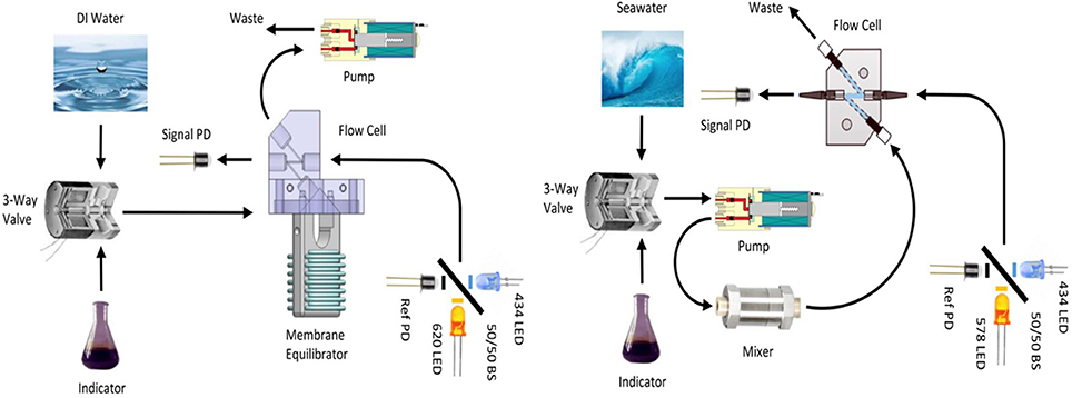
Figure 1. Schematics of current design of (Left) SAMI-CO₂ and (Right) SAMI-pH. The SAMI-pH can be configured with an additional three-way valve at the seawater port to select between the seawater sample and a tris buffer certified reference material (CRM). 50/50 BS, 50% beam-splitter; Signal PD, Signal photodiode; Ref PD, reference photodiode.

Rather than using a commercial photodiode array or CCD spectrograph (e.g., Ocean Optics USB2000), we kept the optical detection system as simple as possible by using individual photodiodes with a custom amplification circuit. In the original SAMI-CO₂ design, light separation was accomplished with a spectrograph with three detectors, including a reference wavelength at 740 nm where the indicator does not absorb light (DeGrandpre et al., 1999). The input fiber optic end face was placed directly against the ~2 mm diameter tungsten lamp bulb with no optics to enhance collection. This simple but relatively low light throughput design required 10⁸ analog amplification to obtain an optimal voltage range for A/D conversion (0–5 V).

Because of the cost and size of the spectrograph and difficulty in accurately setting the detection wavelengths, we converted the detection system to a 1 × 3 fiber optic splitter with interference bandpass and short pass infrared filters (Yuan and DeGrandpre, 2006). Although this design had higher light throughput and better wavelength accuracy than the spectrograph, the coupler-to-coupler splitting ratio was inconsistent. Sometimes one of the channels of the splitter would have very low light intensity and would not be useable.

The current SAMI design uses 2 LEDs (Roithner Lasertechnik) and a beam-splitter that directs light to the optical cell via a fiber optic or to a reference photodiode (Figure 1). For SAMI-CO₂, 435 and 620 nm LEDs are filtered at 436 and 620 nm, respectively, with 10 nm bandpass filters (full width at half-maximum, Intor Inc.). For SAMI-pH, 435 and 575 nm LEDs are filtered at 436 and 578 nm, respectively, also with 10 nm bandpass filters. Light from the alternately pulsed LEDs are combined using a 50:50 beam-splitter (Edmond Optics). Fifty percent of the light is sent to the optical cell through an 800-μm core fused-silica fiber optic (F-MSC-OPT, Newport Corp). Transmitted light is returned via the same sized fiber optic and detected with a photodiode (Hamamatsu Corp.). The other 50% of the light from the beam-splitter passes through a neutral density filter to a reference photodiode. The reference is used to monitor the LED output and correct for source fluctuations in real time (I_λref in Equation 8). In this design, the reference light does not pass through the optical cell as in the previous designs, and therefore transmittance changes through the optical cell and back to the detector are not corrected until a blank is run. We have found that the reference photodiode corrects for small changes in LED output over time, as discussed below. The LED beam-splitter design also has the advantages, relative to the tungsten lamp, of no warm-up time, high light intensity over a narrow wavelength range, and the ability to be electronically modulated to shift the measurement into a low noise area of the frequency spectrum.

SAMI Fluidics Design

The same miniature, low dead-volume solenoid pumps (The Lee Co., Inc.) have been used to pump the solutions since the original design (DeGrandpre et al., 1995). These pumps only require a <1 s voltage pulse to activate the solenoid. The pump in the SAMI-CO₂ is located downstream of the optical cell (Figure 1) to prevent contamination of the indicator solution from leachates in the pump. In the earlier design, we found that the response (R_CO2, Equation 6) depended upon the residence time of the indicator in the flow path. We attributed this time dependence to contamination of the BTB solution, primarily from the pump. The BTB solution is very sensitive to acidic or basic leachates because it must be very weakly buffered to achieve a ~1 μatm sensitivity. The current pump configuration reduces the reagent contamination, but with the trade-off that downstream pumping can pull air through the membrane introducing bubbles into the flow path. While not a problem during deployments under hydrostatic pressures of a few meters of water, bubbles are anathema to optofluidic systems in lab testing at ambient pressures. The z-shaped flow path in the optical cell helps prevent bubbles from sticking at the fiber end-faces. Bubble trapping was worse in the previous design that had the inlet and outlet 90° to the optical path (DeGrandpre et al., 1999, 2000).

The pump and valve are pressure compensated using a silicone oil-filled housing with a rubber diaphragm. The SAMIs have no fundamental depth limitation and the SAMI-pH operated well during the XPRIZE 3,000 m hydrocast tests using a titanium pressure housing. At these depths, however, the BTB and mCP equilibrium constants change significantly. The mCP pressure dependence is known (Soli et al., 2013) and was used in the XPRIZE competition. The BTB pressure dependence is not known and would result in potential calibration errors for deep deployments of the SAMI-CO₂ of ~20 μatm/1,000 m seawater if assumed equal to the mCP pressure dependence.

The SAMI-CO₂ uses 0.16 cm outer diameter (OD) and 0.08 cm internal diameter (ID) high purity fluoroaniline (HPFA) tubing (Idex Health & Science) for all component connections. The membrane equilibrator consists of 1.00 m silicone tubing (0.630 mm OD, 0.300 mm ID). The membrane equilibrator has sufficient volume to flush the downstream optical cell with CO₂-equilibrated solution (~30×, cell volume = 8.5 μL, membrane volume = 282 μL). The total flush volume from the valve to the outlet of the optical cell is ~655 μL. During each measurement cycle, the pump is activated, pulling the CO₂-equilibrated solution into the fiber optic flow cell. The SAMI-CO₂ is operated in a stopped-flow mode so that the seawater CO₂ can equilibrate with the indicator solution (requiring a minimum of 5 min). Because the response is not flow dependent, there is no effect from the pulsatile nature of these pumps. Each measurement sequence consists of 2 pulses of the 50 μL per pulse pump (100 μL of the BTB solution). As stated above, a deionized water blank is periodically flushed through the tubing. This requires 1.2 mL of water (24 pump pulses) and 1.4 mL (28 pump pulses) of reagent to flush the blank. The gas-impermeable reagent bags (Pollution Measurement Corp.) are used to store solutions for the measurements.

The SAMI-pH fluidic layout consists of a simple modification of the SAMI-CO₂ design (Martz et al., 2003; Seidel et al., 2008) (see Figure 1). The normally open valve port, which is connected to the reagent in the SAMI-CO₂, is connected to an inlet tube for the seawater (or freshwater) sample, and the normally closed valve port is connected to the mCP indicator solution in place of the SAMI-CO₂ deionized water blank. A static mixing tube (0.32 cm OD × 14 cm long) replaces the gas-permeable membrane and detection wavelengths are changed to suit mCP. Each SAMI-pH measurement consists of 35 50-μL pump pulses (1.75 mL of sample) through the mixer and optical cell to clear any remaining indicator and fill the system with fresh sample. Then a 50-μL aliquot of indicator is drawn through the normally closed port of the valve and 27 more 50 μL aliquots of sample (1.35 mL) are pumped. Indicator and sample water are mixed along the flow path enroute to the optical flow-cell. At each of these 27 pump cycles an intensity measurement is taken at 434 and 578 nm. The first four of these intensity measurements are used for the blank and are averaged together for a blank intensity, I_λ0 (Equation 8). The SAMI-pH pump and valve housing are configured so that an additional three-way valve can be used to periodically measure a tris CRM pH buffer for in situ data validation if desired. However, we have found that in situ validation is not necessary as the SAMI pH does not drift (Harris et al., 2013). Each SAMI-pH measurement requires 88 W-S, enabling about 5500 measurements with an 8 D-cell battery pack.

The performance parameters for SAMI-CO₂ and SAMI-pH of the current version are summarized in Table 1. The SAMI-CO₂ in situ accuracy can vary depending upon the availability of sample validation and biofouling of the membrane (see below).

TABLE 1

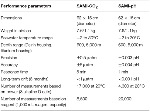
Table 1. Summary of SAMI Performance Parameters.

Evaluations of the SAMI

The tris buffer certified reference material (CRM) solutions were prepared based on a literature recipe (DelValls and Dickson, 1998). Absorbance linearity was tested using different concentrations of bromocresol purple (BCP, lot # MKBQ3276V). Although this is the indicator used in the SAMI alkalinity system (Spaulding et al., 2014), its wavelengths are similar to mCP and it therefore serves to illustrate absorbance accuracy and linearity effects. Absorbance accuracy can degrade at high absorbances due to the presence of light outside of the selected bandpass or due to polychromatic radiation (stray light). As the absorbance increases, the more weakly-absorbed wavelengths become a larger part of the transmitted signal, leading to non-linearity and absorbance inaccuracy. To test this, the pH of the BCP solutions was adjusted using 0.1 N HCl, or 0.1 N NaOH, to convert the indicator to exclusively the acid or base forms of BCP, respectively. The solutions were stored in a sealed bag to prevent pH change due to CO₂ gas exchange.

Results and Discussion

Data are presented from various lab evaluations and field deployments to illustrate the performance characteristics of the SAMI technology. The optical system is first discussed, followed by evaluation of two long-term pH and pCO₂ data sets from the U.S. west coast and Arctic Ocean locations, respectively.

Optical System Evaluation

An ideal optical design for indicator-based absorbance measurements should have high light throughput and low noise with <0.001 absorbance accuracy and linearity over a wide absorbance range. We obtain ~ ±0.0001 absorbance unit precision with the beam-splitter design (Figure 1). This absorbance precision translates into pCO₂ and pH precision of ~ ±0.5 μatm and ~ ±0.0005 pH unit precision, respectively. The SAMI-pH precision degrades to ~ ±0.003 pH units due to noise in the pH perturbation correction (the linear fit to the pH vs. indicator concentration data as described above). Absorbance accuracy and linearity fall off around 1.5 a.u. (absorbance units, see Figure 2) due to stray light. While stray light often originates from near-infrared (NIR) radiation and high Si photodiode sensitivity in the NIR (Yuan and DeGrandpre, 2006), the LEDs have no NIR emission. Rather, the relatively large bandpass results in a variable molar absorption coefficient (Ingle and Crouch, 1988). A stray light contribution of 0.05 and ~0.2% at 590 and 436 nm, respectively, would cause the observed absorbance errors. The larger stray light at the short wavelength might be due to lower overall transmittance and lower detector sensitivity in this part of the spectrum, making the stray light signal a larger component of the total signal. In this design it is best to avoid absorbances greater than ~1.5 because absorbance errors create errors in pH (DeGrandpre et al., 2014) and deviations from the pCO₂ theoretical response.

FIGURE 2

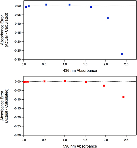
Figure 2. Absorbance linearity of the SAMI optical system at the wavelengths used for BCP in the SAMI alkalinity system (Spaulding et al., 2014). Absorbances were measured for BCP solutions with concentrations ranging from 1.4 × 10⁻⁷ to 3.4 × 10⁻⁵ M at 590 nm (pH = 10.5) and 2.09 × 10⁻⁶ to 1.04 × 10⁻⁴ M at 436 nm (pH = 3.0). A linear fit to absorbance vs. concentration data up to 1.0 a.u. was used and the residuals (y-axis data) were calculated relative to the linear equation.

In Situ Data Evaluation

While the SAMIs have collected time-series data from many different marine and freshwater environments, the analytical performance associated with these deployments has not been a focus. Here we evaluate a SAMI-pH deployment between April and September of 2011 (150 days total) and a SAMI-CO₂ deployment between October 2014 and September 2015 (356 days total). Both instruments were deployed on moorings where no servicing was possible.

The SAMI-pH was deployed on a mooring in the Oregon coastal upwelling zone (Harris et al., 2013). It measured seawater pH every 3 h and a tris buffer sample once every 5 days. The seawater pH ranged between 7.7 and 8.4, with a minimum pH of 7.71 at the beginning of July (Figure 3A). The upwelling of cold, low pH, high CO₂ water created large and rapid changes of pH. The pH changed as much as 0.4 pH units during the most intense upwelling periods.

FIGURE 3

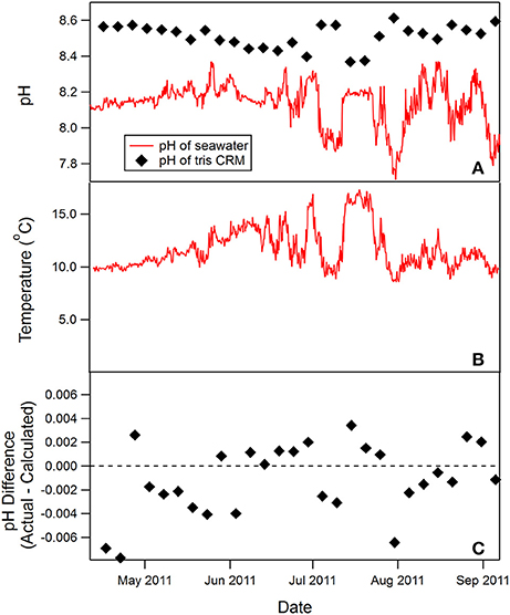
Figure 3. SAMI-pH seawater pH and temperature time-series collected in the surface ocean off the Oregon coast (44.6°N, 124.3°W) in collaboration with Burke Hales (OSU) (A,B). Tris seawater buffer was measured every 5 days during the deployment (black diamonds in A). Tris pH varies due to its strong temperature dependence and is higher at colder temperatures. The difference between the measured and calculated tris pH is shown in (C) (−0.001 ± 0.003 pH units, n = 28).

The tris pH measured in situ during the deployment is compared to the calculated tris pH value using the temperature and salinity-dependent equation for tris buffer (DelValls and Dickson, 1998) (Figure 3A). The tris pH is much higher at the in situ temperature (10–15°C, see Figure 3B) than the seawater pH, however, the measured tris values are within −0.001 ± 0.003 pH units (mean ± SD, n = 28) of the calculated tris pH values and there is no identifiable drift over time (see Figure 3C).

A 1-year pCO₂ time-series collected on a subsurface mooring in the Arctic Ocean (149°59.8203′ W, 78°0.6177′ N) from 2014 to 2015 is shown in Figure 4. The SAMI-CO₂ was located at ~35 m depth. The pCO₂ slowly increased during the winter months followed by a decrease in the spring and summer with occasional large and rapid changes synchronous with rapid changes in temperature. The slow increase and decrease were likely caused by ice exclusion of CO₂ during fall/winter ice formation (e.g., Rysgaard et al., 2007) and possibly biological production in the spring. The rapid changes were caused by large eddies, based on changes in the sensor depths, with different pCO₂ and temperature than the surrounding water. In one case, an eddy laid over the mooring to ~280 m depth (around 09/17/2015). Eddies are common in the Canada Basin and can be distinguished from the surrounding water based on their temperature and salinity characteristics (Timmermans et al., 2008). The pCO₂ levels were not consistent in the eddy water with lower levels found until late in the time-series when the pCO₂ was higher than the surrounding water. A more complete interpretation of these data will be presented in a future manuscript. Although we had limited data for validation, the absorbances and pCO₂ returned to the levels found when the instruments were deployed, completing the annual cycle (most biogeochemical species have similar year to year levels, e.g., Bates, 2017). This observation supports the long-term stability of the SAMI-CO₂ measurements.

FIGURE 4

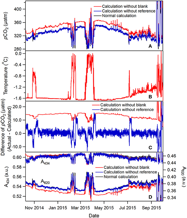
Figure 4. A 1-year time series of pCO₂ and temperature collected by a SAMI-CO₂ on a subsurface mooring (~35 m depth) in the Canada Basin of the Arctic Ocean (78°N, 150°W) (A,B). The rapid and large pCO₂ excursions were caused by pull down of the mooring by large eddies (to as deep as ~280 m). The pCO₂ and absorbance data with and without blank and reference measurement intensity corrections (Equation 8) are also shown (C,D). See text for more discussion. The normal calculation values (black curves) are hidden under the calculation without reference (blue curves).

These in situ time-series data show how blank and reference intensity (both I_λ0 and I_λ0ref in Equation 8) correct for light source and transmittance variability. Similar corrections have been reported in other optofluidic sensors to achieve better accuracy and reduce drift (Grand et al., 2017). The pCO₂ calculated using blank and reference intensity corrections (named “normal calculation” as mentioned later or in figures) is compared with pCO₂ calculated using absorbances without these corrections [i.e., using a constant I_λ0 or setting log(I_λref/I_λ0ref) equal to zero in Equation 8]. For the data shown in Figure 4, the calculated pCO₂ without the blank correction would result in an error in the range of +5 to +43 μatm. There is a significant mean offset if no blank is used primarily due to a change in transmittance of light at 620 nm (Figure 4D). Transmittance changes occurred between the calibration, in this case conducted at the University of Montana on April 29, 2014, shipment via truck and research vessel to the deployment site, and subsequent deployment into near freezing seawater. It should be noted that, we have never had issues with reagents freezing. For SAMI-pH, the reagents used in the deployment were made to match the salinity background of seawater by adding NaCl salt to salinity 35. The increased concentration of solute therefore decreased the freezing point. For SAMI-CO₂, ethylene glycol is added in reagents to avoid freezing. Moreover, the time on deck is kept to a minimum during the mooring deployments. After the initial offset, the offset remained essentially the same and there is very little correction afforded by running blanks, likely due to the very small temperature variability (<1.7°C) in this location (Figure 4B). Regular blank measurements are still recommended to correct temperature related blank errors during a deployment but a smarter blank measurement could be implemented that is run only when temperature exceeds a certain threshold.

The reference correction I_λ0ref is sometimes significant, particularly when the temperature changes significantly between blank periods (see the spikes in the blue curve in Figure 4C). The reference in this case is primarily accounting for temperature dependent changes in the LED output intensity between blanks based on the coinciding pCO₂ offsets and rapid changes in temperature. The calculated pCO₂ without the reference signal correction would result in periodic errors ranging from −12 to +83 μatm (Equation 8). The offsets disappear when a new blank intensity is obtained. The reference signal also corrects for random noise in the LED signal (compare the calculations without blank and without reference in Figure 4C). A ~ ±2 μatm pCO₂ noise is present without the reference. The high noise level is not normal and the cause is unknown.

An expanded period from Figure 4, when pCO₂ was relatively stable, more clearly shows the absorbance and pCO₂ precision (Figure 5). The absorbances at both wavelengths changed less than 0.005 a.u. during this period and the precision (determined based on the raw absorbance data) is much less than ±0.001 a.u. due to the high optical throughput and referencing, as discussed above. This absorbance precision leads to pCO₂ precision less than 1 μatm. Also notable are the occasional small spikes in absorbance, most evident at 434 nm, that lead to regular pCO₂ spikes (e.g., from May to July, Figure 4D). These anomalous changes occur due to inadequate flushing of the deionized water blank. After the blank is flushed with indicator solution, some of the water remains in poorly flushed dead volume areas, that then dilutes and alters the pH of the BTB solution for 1 or 2 subsequent measurements (Figure 5). The spikes are slightly delayed after the blank because the first couple of measurements use BTB solution that resided in tubing not affected by the blank. This problem highlights the importance of dead volumes in optofluidic plumbing particularly when dilute, poorly buffered reagents are used.

FIGURE 5

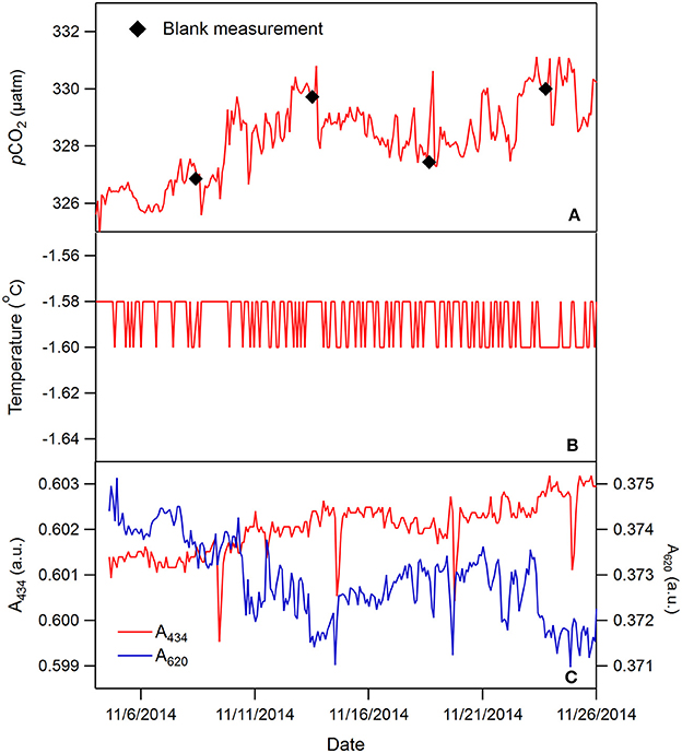
Figure 5. An expanded ~22-day period from Figure 4 showing blank flushing effects. The temperature was essentially constant and below the resolution of the thermistor probe (B). The absorbances at 434 and 620 nm are shown (C). See text for more discussion.

Reliability

There are many possible sources of failure in any autonomous sensing system ranging from fish bites, biofouling (see below), electronic or battery failure, leaking seals, software glitches, failure to turn on the instrument (i.e., user errors) and others. Pumping small volumes of liquids pose their own unique set of problems some of which have been highlighted above. In the SAMIs, pumps and valves are the most common source of failure. It is often difficult to diagnose why a pump fails but clogged tubing, stuck check valves, inadequate pressure compensation, dried reagent, or salts and pump air-locks are the most common problems that we have encountered. The pump and valve housing must be fully filled with pressure compensating liquid (silicone oil in this case) or the diaphragm might not have sufficient range to make up for the missing volume. One difference between the SAMI-CO₂ and SAMI-pH is that the SAMI-pH will pump air into its tubing when it is not submerged. If the instrument is deployed at depths > ~5 m, air in the pump will collapse the check valves and no liquid can be drawn in. Consequently, a bag of water is always attached to the SAMI-pH inlet and removed just before deployment. This is not a problem we have encountered with the SAMI-CO₂ because it is a closed system (it always draws from a bag of reagent or bag of deionized water, see Figure 1). The liquid in the membrane can evaporate when not in use, however, but benchtop pumping prior to deployment can refill the system. Other pump and valve designs will no doubt have their own unique failure mechanisms and therefore need to be lab tested for long periods under representative pressures and temperatures.

Biofouling

There is no innate sensitivity of the SAMI technology to biofouling relative to other sensors but we provide this discussion to aid other researchers who utilize optofluidic or other in situ analyzers. Biofouling sensitivity could appear as a local signal due to concentrated heterotrophs (e.g., barnacles) or autotrophs (e.g., macroalgae), or generation of particulate matter that causes clogging of the inlet or outlet tubing, or interferes with the light transmittance in the optical cell. The latter effects can occur in highly productive coastal waters with high particulate matter concentrations. The small ID tubing and low flow rates make it difficult to draw particulates into the flow path and we also use 10 μm PTFE filters at SAMI-pH inlet to prevent internal fouling and signal degradation. In the case of biological growth, it is very difficult to diagnose localized generation or loss of CO₂ due to photosynthesis or respiration unless the local biological signal becomes so large that the levels becomes unrealistic. Consequently, it is to be avoided as much as possible. We do this by relying on technology proven for Sea-Bird Electronics' conductivity sensors—i.e., isolating the sensor in an enclosed cell that is periodically flushed with sample that has been exposed to a biocide such as tributyl tin or copper (Figure 6). Fouling issues like these also affect dissolved O₂ optodes, which also have gas permeable membranes. Copper mesh is used to protect from fish bites and other sources of damage (e.g., during deployment) because any other material provides a lattice for algal growth (Figure 6). Copper tape around the instrument has also proven useful in keeping biofouling to a minimum.

FIGURE 6

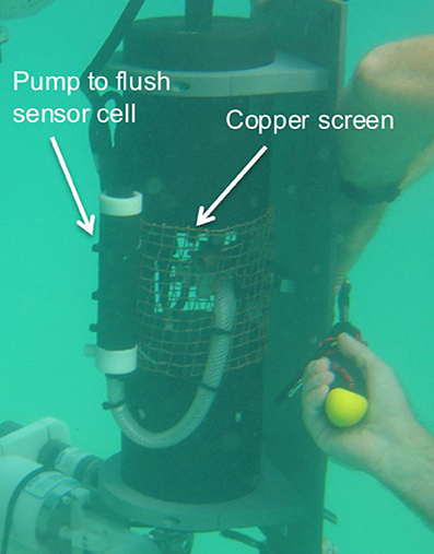
Figure 6. A SAMI-CO₂ with an anti-fouling configuration. The membrane equilibrator (Figure 1) is enclosed in a flow cell that isolates it from the seawater. Either a tributyl tin plug or a copper inlet tubing is used as antifouling agents to prevent fouling in the enclosed cell. The copper screen is used as a protective enclosure that also discourages biofouling around the sensor area.

Conclusions and Perspectives

The optofluidic designs shown here offer insights into the pros and cons of using pumps and valves for reagent based sensing. As we have shown, pumping makes it possible to re-establish the optical baseline, a necessity to achieve the accuracy required for autonomous, calibration-free measurements. In situ pCO₂ measurements are particularly difficult to calibrate because no reliable liquid standard exists. Other optofluidic systems, however, can use calibration standards to correct for various sources of drift (e.g., Beaton et al., 2012; Grand et al., 2017). One way to avoid the additional complexity of pumping is to use fluorescent lifetime based measurements that have reduced sensitivity to the signal intensity. This technology has been successfully developed for dissolved O₂ sensors (Körtzinger et al., 2005; Tengberg et al., 2006; Takeshita et al., 2013), while similar technology for pH and pCO₂ has proven more challenging but recent developments show promise in field deployments (Atamanchuk et al., 2014; Clarke et al., 2015; Fritzsche et al., 2017).

Clearly there is no single technological route to develop reliable, low power, accurate, and precise marine biogeochemical sensors. Many chemical species will not be measurable by time-domain fluorescence sensing or electrochemical transducers and more complex optofluidic sensing with reagent chemistries are required. Many of the current optofluidic marine sensors are considerably more complex than the SAMI technology described here (e.g., Beaton et al., 2012) due to their more complicated chemistries. Innovations, such as using a tracer to quantify addition of titrant in an alkalinity titration, can make it possible to simplify fluidic designs (Martz et al., 2006). Microfluidic technology offers minimal reagent consumption, the possibility of simple snap together, tubeless assemblies, with integrated pumps and valves but whether they will create other technical challenges (e.g., clogging, reagent contamination, poor optical throughput), remains to be seen.

Author Contributions

C-ZL and MD shared in the writing. C-ZL led the data processing. RD helped with figures and writing.

Funding

Early funding to develop the SAMI-CO₂ came from the U.S. Department of Energy Ocean Margins Program and the National Science Foundation (NSF) Ocean Technology Program. The National Oceanographic Partnership Program provided funding to commercialize the SAMI-CO₂ and SAMI-pH. NSF and NOAA have supported using the SAMIs for scientific research applications. The Arctic data were collected as part of the NSF Arctic Observing Network program (ARC-1107346, PLR-1504410).

Conflict of Interest Statement

MD is a co-owner of Sunburst Sensors, LLC, the company that manufactures the SAMI instruments.

The other authors declare that the research was conducted in the absence of any commercial or financial relationships that could be construed as a potential conflict of interest.

Acknowledgments

James Beck (Sunburst Sensors), Terence Hammar (Woods Hole Oceanographic Institution), and Cory Beatty (University of Montana) have all made important contributions to the development of the SAMI technology. We also thank MD's research group at the University of Montana and Sunburst Sensors personnel, especially Adam Prody (UM) who provided the BCP linearity data. Mooring deployments discussed here were made possible through collaborations with Burke Hales (Oregon State University) and Rick Krishfield and Andrey Proshutinsky (Woods Hole Oceanographic Institution).

References

Atamanchuk, D., Tengberg, A., Thomas, P. J., Hovdenes, J., Apostolidis, A., Huber, C., et al. (2014). Performance of a lifetime-based optode for measuring partial pressure of carbon dioxide in natural waters. Limnol. Oceanogr. Methods 12, 63–73. doi: 10.4319/lom.2014.12.63

CrossRef Full Text | Google Scholar

Bagshaw, E. A., Beaton, A. D., Wadham, J. L., Mowlem, M. C., Hawkings, J. R., and Tranter, M. (2016). Chemical sensors for in situ data collection in the cryosphere. Trends Analyt. Chem. 82, 348–357. doi: 10.1016/j.trac.2016.06.016

CrossRef Full Text | Google Scholar

Bates, N. R. (2017). Twenty years of marine carbon cycle observations at devils hole Bermuda provide insights into seasonal hypoxia, coral reef calcification, and ocean acidification. Front. Mar. Sci. 4:36. doi: 10.3389/fmars.2017.00036

CrossRef Full Text | Google Scholar

Beaton, A. D., Cardwell, C. L., Thomas, R. S., Sieben, V. J., Legiret, F.-E., Waugh, E. M., et al. (2012). Lab-on-chip measurement of nitrate and nitrite for in situ analysis of natural waters. Environ. Sci. Technol. 46, 9548–9556. doi: 10.1021/es300419u

PubMed Abstract | CrossRef Full Text | Google Scholar

Clarke, J. S., Achterberg, E. P., Rerolle, V. M. C., Abi Kaed Bey, S., Floquet, C. F. A., and Mowlem, M. C. (2015). Characterisation and deployment of an immobilised pH sensor spot towards surface ocean pH measurements. Anal. Chem. Acta 897, 69–80. doi: 10.1016/j.aca.2015.09.026

PubMed Abstract | CrossRef Full Text | Google Scholar

Clayton, T. D., and Byrne, R. H. (1993). Spectrophotometric seawater pH measurements: total hydrogen ion concentration scale calibration of m-cresol purple and at-sea results. Deep Sea Res. Pt I 40, 2115–2129. doi: 10.1016/0967-0637(93)90048-8

CrossRef Full Text | Google Scholar

DeGrandpre, M. D. (1993). Measurement of seawater pCO₂ using a renewable-reagent fiber optic sensor with colorimetric detection. Anal. Chem. 65, 331–337. doi: 10.1021/ac00052a005

CrossRef Full Text | Google Scholar

DeGrandpre, M. D., Baehr, M. M., and Hammar, T. R. (1999). Calibration-free optical chemical sensors. Anal. Chem. 71, 1152–1159. doi: 10.1021/ac9805955

CrossRef Full Text | Google Scholar

DeGrandpre, M. D., Baehr, M. M., and Hammar, T. R. (2000). “Development of an optical chemical sensor for oceanographic applications: the submersible autonomous moored instrument for seawater CO₂,” in Chemical Sensors in Oceanography, ed M. S. Varney (Amsterdam: Gordon and Breach publisher), 123–141.

Google Scholar

DeGrandpre, M. D., Hammar, T. R., Smith, S. P., and Sayles, F. L. (1995). In situ measurements of seawater pCO₂. Limnol. Oceanogr. 40, 969–975. doi: 10.4319/lo.1995.40.5.0969

CrossRef Full Text | Google Scholar

DeGrandpre, M. D., Hammar, T. R., Wallace, D. W. R., and Wirick, C. D. (1997). Simultaneous mooring-based measurements of seawater CO₂ and O₂ off Cape Hatteras, North Carolina. Limnol. Oceanogr. 42, 21–28. doi: 10.4319/lo.1997.42.1.0021

CrossRef Full Text | Google Scholar

DeGrandpre, M. D., Spaulding, R. S., Newton, J. O., Jaqueth, E. J., Hamblock, S. E., Umansky, A. A., et al. (2014). Consideration for the measurement of spectrophotometric pH for ocean acidification and other studies. Limnol. Oceanogr. Methods 12, 830–839. doi: 10.4319/lom.2014.12.830

CrossRef Full Text | Google Scholar

DelValls, T. A., and Dickson, A. G. (1998). The pH of buffers based on 2-amino-2-hydroxymethyl-1,3-propanediol (tris) in synthetic sea water. Deep Sea Res. Pt I 45, 1541–1554. doi: 10.1016/S0967-0637(98)00019-3

CrossRef Full Text | Google Scholar

Fritzsche, E., Gruber, P., Schutting, S., Fischer, J. P., Strobl, M., Müller, J. D., et al. (2017). Highly sensitive poisoning-resistant optical carbon dioxide sensors for environmental monitoring. Anal. Methods 9, 55–65. doi: 10.1039/C6AY02949C

CrossRef Full Text | Google Scholar

Grand, M. M., Clinton-Bailey, G. S., Beaton, A. D., Schaap, A. M., Johengen, T. H., Tamburri, M. N., et al. (2017). A lab-on-chip phosphate analyzer for long-term in situ monitoring at fixed observatories: optimization and performance evaluation in estuarine and oligotrophic coastal waters. Front. Mar. Sci. 4:255. doi: 10.3389/fmars.2017.00255

CrossRef Full Text | Google Scholar

Harris, K. E., DeGrandpre, M. D., and Hales, B. (2013). Aragonite saturation state dynamics in a coastal upwelling zone. Geophys. Res. Lett. 40, 2720–2725. doi: 10.1002/grl.50460

CrossRef Full Text | Google Scholar

Ingle, J. D. J., and Crouch, S. R. (1988). Spectrochemical Analysis. Englewood Cliffs, NJ: Old Tappan.

Google Scholar

Johnson, K. S., Beehler, C. L., and Sakamoto-Arnold, C. M. (1986a). A submersible flow analysis system. Anal. Chim. Acta 179, 245–257.

Google Scholar

Johnson, K. S., Beehler, C. L., Sakamoto-Arnold, C. M., and Childress, J. J. (1986b). In situ measurements of chemical distributions in a deep-sea hydrothermal vent field. Science 231, 1139–1141.

PubMed Abstract | Google Scholar

Johnson, K. S., and Coletti, L. J. (2002). In situ ultraviolet spectrophotometry for high resolution and long-term monitoring of nitrate, bromide and bisulfide in the ocean. Deep Sea Res. Pt I 49, 1291–1305. doi: 10.1016/S0967-0637(02)00020-1

CrossRef Full Text | Google Scholar

Körtzinger, A., Schimanski, J., and Send, U. (2005). High quality oxygen measurements from profiling floats: a promising new technique. J. Atmos. Ocean. Tech. 22, 302–308. doi: 10.1175/JTECH1701.1

CrossRef Full Text | Google Scholar

Liu, X., Patsavas, M. C., and Byrne, R. H. (2011). Purification and characterization of meta-cresol purple for spectrophotometric seawater pH measurements. Environ. Sci. Technol. 45, 4862–4868. doi: 10.1021/es200665d

PubMed Abstract | CrossRef Full Text | Google Scholar

Martz, T. R., Carr, J. J., French, C. R., and DeGrandpre, M. D. (2003). A submersible autonomous sensor for spectrophotometric pH measurements of natural waters. Anal. Chem. 75, 1844–1850. doi: 10.1021/ac020568l

PubMed Abstract | CrossRef Full Text | Google Scholar

Martz, T. R., Connery, J. G., and Johnson, K. S. (2010). Testing the Honeywell Durafet® for seawater pH applications. Limnol. Oceanogr. Methods 8, 172–184. doi: 10.4319/lom.2010.8.172

CrossRef Full Text | Google Scholar

Martz, T. R., Dickson, A. G., and DeGrandpre, M. D. (2006). Tracer monitored titrations: measurement of total alkalinity. Anal. Chem. 78, 1817–1826. doi: 10.1021/ac0516133

PubMed Abstract | CrossRef Full Text | Google Scholar

Nightingale, A. M., Beaton, A. D., and Mowlem, M. C. (2015). Trends in microfluidic systems for in situ chemical analysis of natural waters. Sens. Actuators B 221, 1398–1405. doi: 10.1016/j.snb.2015.07.091

CrossRef Full Text | Google Scholar

Okazaki, R. R., Sutton, A. J., Feely, R. A., Dickson, A. G., Alin, S. R., Sabine, C. L., et al. (2017). Evaluation of marine pH sensors under controlled and natural conditions for the Wendy Schmidt ocean health XPRIZE. Limnol. Oceanogr. Methods 15, 586–600. doi: 10.1002/lom3.10189

CrossRef Full Text | Google Scholar

Rerolle, V. M. C., Floquet, C. F. A., Harris, A. J. K., Mowlem, M. C., Bellerby, R. R. G. J., and Achterberg, E. P. (2013). Development of a colorimetric microfluidic pH sensor for autonomous seawater measurements. Anal. Chim. Acta 786, 124–131. doi: 10.1016/j.aca.2013.05.008

PubMed Abstract | CrossRef Full Text | Google Scholar

Rysgaard, S., Glud, R. N., Sejr, M. K., Bendtsen, J., and Christensen, P. B. (2007). Inorganic carbon transport during sea ice growth and decay: a carbon pump in polar seas. J. Geophys. Res. 112:C03016. doi: 10.1029/2006JC003572

CrossRef Full Text | Google Scholar

Schmidt, M., Linke, P., and Esser, D. (2013). Recent development in IR sensor technology for monitoring subsea methane discharge. Mar. Technol. Soc. J. 47, 27–36. doi: 10.4031/MTSJ.47.3.8

CrossRef Full Text | Google Scholar

Seidel, M. P., DeGrandpre, M. D., and Dickson, A. G. (2008). A sensor for in situ indicator-based measurements of seawater pH. Mar. Chem. 109, 18–28. doi: 10.1016/j.marchem.2007.11.013

CrossRef Full Text | Google Scholar

Soli, A. L., Pav, B. J., and Byrne, R. H. (2013). The effect of pressure on meta-cresol purple protonation and absorbance characteristics for spectrophotometric pH measurements in seawater. Mar. Chem. 157, 162–169. doi: 10.1016/j.marchem.2013.09.003

CrossRef Full Text | Google Scholar

Spaulding, R. S., DeGrandpre, M. D., Beck, J. C., Hart, R. D., Peterson, B., De Carlo, E. H., et al. (2014). Autonomous in situ measurements of seawater alkalinity. Environ. Sci. Technol. 48, 9573–9581. doi: 10.1021/es501615x

PubMed Abstract | CrossRef Full Text | Google Scholar

Sutton, A. J., Sabine, C. L., Maenner-Jones, S., Lawrence-Slavas, N., Meinig, C., Feely, R. A., et al. (2014). A high-frequency atmospheric and seawater pCO₂ data set from 14 open-ocean sites using a moored autonomous system. Earth Syst. Sci. Data 6, 353–366. doi: 10.5194/essd-6-353-2014

CrossRef Full Text | Google Scholar

Takeshita, Y., Martz, T. R., Johnson, K. S., Plant, J. N., Gilbert, D., Riser, S. C., et al. (2013). A climatology based quality control procedure for profiling float oxygen data. J. Geophys. Res. Oceans 118, 5640–5650. doi: 10.1002/jgrc.20399

CrossRef Full Text | Google Scholar

Tengberg, A., Hovdenes, J., Andersson, H. J., Brocandel, O., Diaz, R., Hebert, D., et al. (2006). Evaluation of a lifetime based optode to measure oxygen in aquatic systems. Limnol. Oceanogr. Methods 4, 7–17. doi: 10.4319/lom.2006.4.7

CrossRef Full Text | Google Scholar

Timmermans, M. L., Toole, J., Proshutinsky, A., Krishfield, R., and Plueddemann, A. (2008). Eddies in the Canada basin, Arctic ocean, observed from ice-tethered profilers. J. Phys. Oceanogr. 38, 133–145. doi: 10.1175/2007JPO3782.1

CrossRef Full Text | Google Scholar

Yuan, S., and DeGrandpre, M. D. (2006). Comparison between two detection systems for fiber-optic chemical sensor applications. Appl. Spectrosc. 60, 465–470. doi: 10.1366/000370206776593591

PubMed Abstract | CrossRef Full Text | Google Scholar