Producing Distribution Maps for a Spatially-Explicit Ecosystem Model Using Large Monitoring and Environmental Databases and a Combination of Interpolation and Extrapolation

Introduction

Ecosystem simulation models are valuable tools for understanding the impacts of environmental and anthropogenic stressors on marine ecosystems and for informing resource management (Fulton, 2010; Christensen and Walters, 2011; O'Farrell et al., 2017). A wide diversity of ecosystem modeling platforms is now available, including the spatially-explicit modeling frameworks Atlantis (Fulton et al., 2004, 2007, 2011), Ecopath with Ecosim with Ecospace (Pauly et al., 2000; Christensen and Walters, 2004; Walters et al., 2010) and OSMOSE (Shin and Cury, 2001, 2004; Grüss et al., 2016c). The simulation of predator-prey interactions is a key feature of ecosystem models (Plaganyi, 2007; Christensen and Walters, 2011; Grüss et al., 2016a). To simulate predator-prey interactions, spatially-explicit ecosystem models need to represent patterns of spatial overlap between predators and prey. To be able to represent patterns of spatial overlap between predators and prey, many spatially-explicit ecosystem modeling platforms, including Atlantis and OSMOSE, need to be provided with distribution maps defining the annual or seasonal spatial distributions of functional groups¹ and life stages.

The extrapolation of spatial distribution patterns predicted by statistical models integrating environmental covariates (commonly called “species distribution models”) is a useful means to produce distribution maps for spatially-explicit ecosystem models (Drexler and Ainsworth, 2013; Grüss et al., 2014, 2016d; Hattab et al., 2014). For example, Drexler and Ainsworth (2013) fitted generalized additive models (GAMs) to monitoring data collected in the U.S. Gulf of Mexico (GOM). The authors then extrapolated the predictions made by their GAMs to the entire GOM Large Marine Ecosystem (LME) to obtain distribution maps for some of the functional groups (all life stages combined) represented in the Atlantis model of the GOM LME (“Atlantis-GOM”; Figure 1). While Drexler and Ainsworth's (2013) methodology is more sophisticated than usual methodologies for generating distribution maps for ecosystem models, it has some limitations. Firstly, Drexler and Ainsworth (2013) employed only one groundfish trawl survey dataset to produce all their distribution maps, which resulted in unreliable predictions of spatial distributions for those functional groups that are poorly sampled by groundfish trawl (e.g., some of the pelagic functional groups represented in Atlantis-GOM). Secondly, Drexler and Ainsworth (2013) used the same set of environmental covariates (dominant sediment type, bottom depth, bottom temperature, bottom dissolved oxygen (DO) concentration, and surface chlorophyll-a concentration) in all their GAMs; however, other environmental parameters may have a stronger influence of the spatial distribution patterns of the functional groups represented in Atlantis-GOM (e.g., sea surface temperature (SST) in the case of most pelagic functional groups). Lastly, Drexler and Ainsworth's (2013) GAMs did not account for spatial autocorrelation (spatial structure), because their purpose was to be employed for performing extrapolation over the entire GOM LME; this led to significant, unmodeled spatial patterns in Drexler and Ainsworth's (2013) GAM residuals for functional groups associated with small-scale habitat features, such as red grouper (Epinephelus morio) and gag (Mycteroperca microlepis) (unpublished data).

FIGURE 1

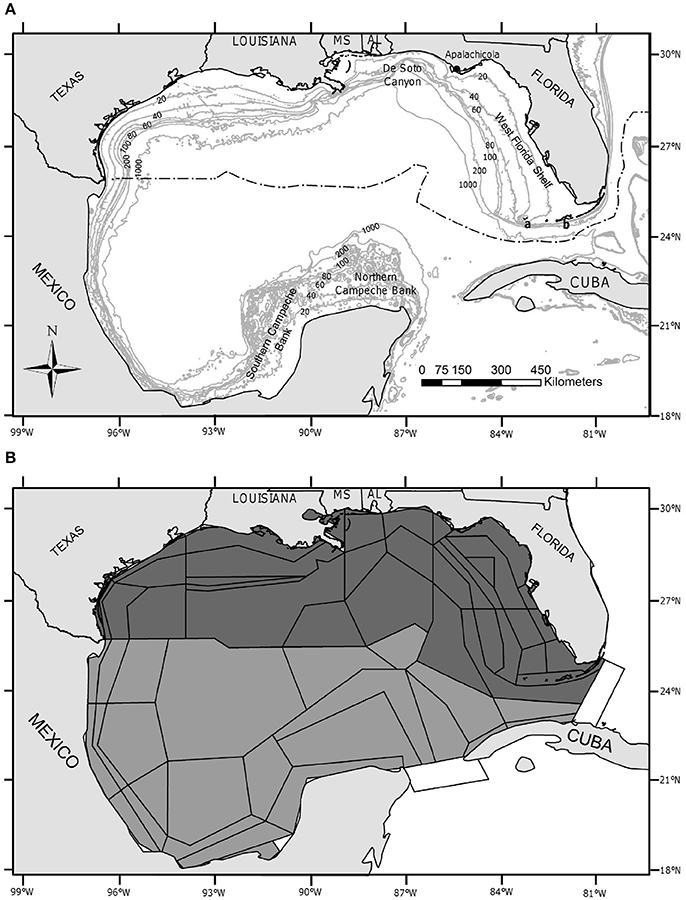
Figure 1. Study area. (A) Map of the Gulf of Mexico Large Marine Ecosystem. Depth contours are labeled in 20-, 40-, 60-, 80-, 100-, 200-, and 1,000-m contours. Important features are labeled and include: the northern Campeche Bank, the southern Campeche Bank, the De Soto canyon, the West Florida Shelf, the Dry Tortugas (A), and the Florida Keys (B). MS, Mississippi; AL, Alabama. The black dashed-dotted line delineates the U.S. exclusive economic zone. (B) Spatial polygons of the Atlantis model of the Gulf of Mexico (GOM) referred to as “Atlantis-GOM”. Atlantis-GOM polygons located in U.S. GOM are filled in dark gray, while those located outside the U.S. GOM (i.e., in the Mexican or Cuban GOM or in international waters) are filled in lighter gray. The two “boundary polygons” of Atlantis-GOM, which do not interact with the rest of the model, are filled in white.

Interpolation from the predictions of geostatistical models is a means to account for spatial structure in spatial distribution patterns (Guisan and Zimmermann, 2000; Saul et al., 2013; Thorson et al., 2015; Grüss et al., 2017b). For instance, Grüss et al. (2017b) fitted geostatistical binomial generalized linear mixed models (GLMMs) to a blending of fisheries-dependent and fisheries-independent monitoring data collected in the U.S. GOM. The authors then interpolated geostatistical GLMM predictions to a spatial grid covering the entire U.S. GOM to be able to generate distribution maps for an OSMOSE model of the West Florida Shelf. Geostatistical binomial GLMMs accurately reflect the probability of encountering functional groups/life stages in a marine ecosystem. However, these models cannot be used to interpolate the spatial distributions of functional groups/life stages over the entire GOM LME, due to the scarcity or limited access to monitoring data collected in the southern GOM (i.e., the Mexican and Cuban GOM and the international waters of the GOM).

To address the above mentioned issues, we developed a novel methodology combining extrapolation and interpolation of the predictions made by statistical habitat models to produce distribution maps for the fish and invertebrates represented in the Atlantis-GOM ecosystem model. This methodology consists of fitting binomial GAMs to a large monitoring database for the U.S. GOM and a large environmental database for the GOM LME, and geostatistical binomial GLMMs to the large monitoring database for the U.S. GOM; and then employing GAM predictions to infer fish and invertebrate spatial distributions in the southern GOM, and geostatistical GLMM predictions to infer fish and invertebrate spatial distributions in the U.S. GOM. The large monitoring database we compiled for the U.S. GOM gathers all the fisheries-dependent and fisheries-independent monitoring data collected in the region between 2000 and 2016 using random sampling schemes. Our large environmental database gathers all the environmental parameters known to influence the spatial distributions of fish and invertebrates of the GOM that are available for both the U.S. and the southern GOM. Thus, our methodology allows for reasonable extrapolation in the southern GOM based on a large amount of monitoring and environmental data, and for interpolation in the U.S. GOM accurately reflecting the probability of encountering fish and invertebrates in that region. Though initially designed for the GOM, our methodology can serve other regions of the world characterized by a large surface area and only partially covered by available monitoring data, such as LMEs bordered by several countries (e.g., the Benguela Current LME).

We present our methodology, which allowed us to construct a total of 116 annual and seasonal distribution maps for the fish and invertebrate functional groups and life stages represented in the Atlantis-GOM ecosystem model. We first briefly present the GOM LME and the Atlantis-GOM model. Then, we provide an overview of our methodology. Next, we describe the compilation of the large monitoring database for the U.S GOM and of the large environmental database for the GOM LME. Afterwards, we explain how we developed and evaluated binomial GAMs for the entire GOM LME and geostatistical binomial GLMMs for the U.S. GOM. Finally, we combine GAM predictions and geostatistical GLMM predictions according to our methodology to generate distribution maps for the fish and invertebrates represented in Atlantis-GOM.

Materials and Methods

The GOM LME and the Atlantis-GOM Ecosystem Model

The GOM is one of the world's 64 LMEs (NOS, 2008). It is bounded on the north by the U.S., and on the south by Mexico and Cuba (Figure 1). Five U.S. States border the U.S. GOM: Florida, Alabama, Mississippi, Louisiana, and Texas. The spatial domain of the Atlantis-GOM ecosystem model covers the entire GOM LME, including the U.S. GOM, the Mexican GOM, the Cuban GOM, and the international waters of the GOM (Figure 1).

Atlantis is a three-dimensional, biogeochemical, and trophic modeling platform, which represents organisms from marine bacteria to apex predators (Fulton et al., 2004, 2007, 2011). Atlantis characterizes biogeography using irregular three-dimensional polygons, which can provide high spatial resolution in key areas while minimizing computation time in homogeneous space. The modeling platform utilizes a biological sub-model that simulates nutrient, detritus and microbial cycles as well as species ecology, and a human impacts sub-model which can represent a wide variety of fisheries activities by modeling direct and indirect functional group mortality and habitat impacts. The distribution maps and vertical distribution profiles fed into Atlantis allow the modeling platform to allocate the biomasses of functional groups and life stages in the horizontal and vertical dimension, respectively (Grüss et al., 2016a).

The Atlantis-GOM model comprises 39 polygons for the U.S. GOM and 24 polygons for the southern GOM, as well as two “boundary polygons”, which do not interact with the rest of the model (Figure 1; Ainsworth et al., 2015). Atlantis-GOM explicitly considers 91 functional groups, including four marine mammals, two seabirds, three sea turtles, 48 fish groups, 15 invertebrate groups (of which three are filter feeders), four structural species, two zooplankton groups, eight primary producers (of which four are phytoplankton groups), and four nutrient cyclers (Supplementary Table 1). In the present study, we focus on the 63 fish and invertebrate functional groups represented in Atlantis-GOM (Table 1). We identified a reference species for each of these 63 functional groups. The identification of reference species was only meant to facilitate literature reviews for functional groups (see subsections Compilation of a Large Monitoring Database for the U.S. GOM and Compilation of a Large Environmental Database for the GOM LME), and data extraction and statistical model fitting considered all the species making up each of the functional groups.

TABLE 1

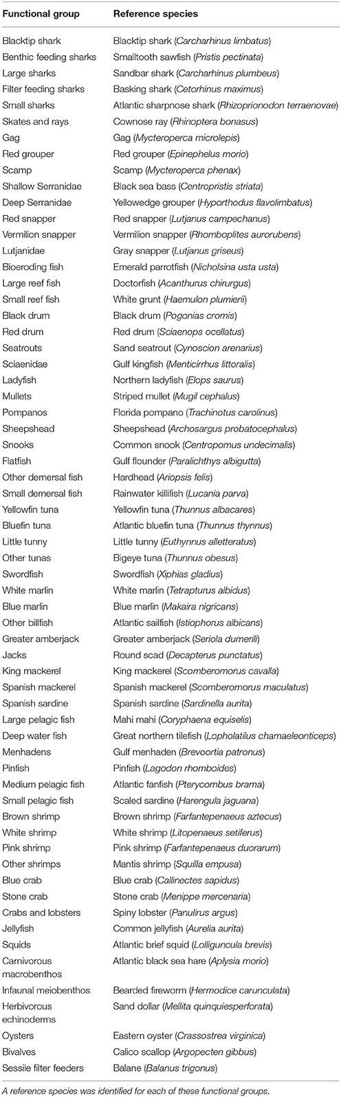
Table 1. Fish and invertebrate functional groups represented in the Atlantis-GOM ecosystem model.

Overview of the Methodology Developed in the Present Study

To produce distribution maps for the fish and invertebrates represented in the Atlantis-GOM ecosystem model at different seasons, we proceeded in six steps (Figure 2).

FIGURE 2

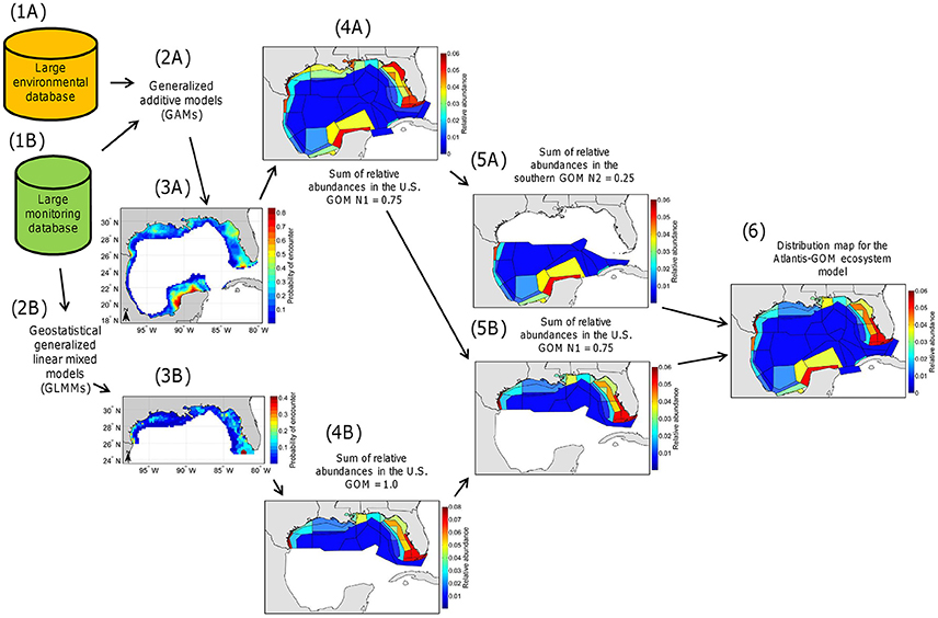
Figure 2. Schematic overview of the methodology developed and employed in the present study. (Step 1A) Construction of a large environmental database for the Gulf of Mexico (GOM) Large Marine Ecosystem (LME). (Step 1B) Construction of a large monitoring database for the northern (U.S.) GOM. (Step 2A) Fitting of binomial generalized additive models (GAMs) to the large environmental and monitoring databases and validation of the GAMs. (Step 2B) Fitting of geostatistical binomial generalized linear mixed models (GLMMs) to the large monitoring database and validation of the geostatistical GLMMs. (Step 3A) Production of long-term probability of encounter maps from GAM predictions. (Step 3B) Production of long-term probability of encounter maps from geostatistical GLMM predictions. (Step 4A) Production of maps of relative abundance for the GOM LME from the maps produced in Step 3A (such that the sum of relative abundances for each map is equal to 1.0). In this example, the sum of relative abundances in the U.S. GOM is equal to N1 = 0.75 and the sum of relative abundances in the southern GOM is equal to N2 = 0.25. (Step 4B) Production of maps of relative abundance for the U.S. GOM from the maps produced in Step 3B (such that the sum of relative abundances for each map is equal to 1.0). (Step 5A) Production of maps of relative abundance for the southern GOM from the maps produced in Step 4A (such that, in this example, the sum of relative abundances for the map for the southern GOM is equal to N2 = 0.25). (Step 5B) Production of maps of relative abundance for the U.S. GOM from the maps produced in Step 4B, rescaled to account for relative abundance in the U.S. GOM relative to the southern GOM according to the map produced in Step 4A (such that, in this example, the sum of relative abundances for the map for the U.S. GOM is equal to N1 = 0.75). (Step 6) Combination of the maps of relative abundance for the southern and U.S. GOM to generate distribution maps usable in the Atlantis-GOM ecosystem model (such that the sum of relative abundances for each distribution map for Atlantis-GOM is equal to 1.0).

First, we compiled a large monitoring database including data collected for fish and invertebrates by monitoring programs of the U.S. GOM over the period 2000–2016 (subsection Compilation of a Large Monitoring Database for the U.S. GOM; Step 1A in Figure 2), and a large environmental database for the GOM LME (subsection Compilation of a Large Environmental Database for the GOM LME; Step 1B in Figure 2).

Second, we fitted binomial GAMs to the large monitoring and environmental databases and validated these GAMs (subsection Development and Evaluation of Binomial GAMs; Step 2A in Figure 2), and we also fitted geostatistical binomial GLMMs to the large monitoring database and validated these geostatistical GLMMs (subsection Development and Evaluation of Geostatistical Binomial GLMMs; Step 2B in Figure 2). Binomial GAMs and geostatistical binomial GLMMs predict the probability of encountering the fish and invertebrate functional groups and life stages represented in the Atlantis-GOM model in the GOM LME and the U.S. GOM, respectively.

Third, we employed fitted binomial GAMs to generate 0.18° × 0.18° (20 × 20 km) long-term probability of encounter maps for the GOM LME (subsection Production of Distribution Maps for the GOM LME from the Predictions Made by Fitted Binomial GAMs; Step 3A in Figure 2), and used the fitted geostatistical binomial GLMMs to generate 20 × 20 km long-term probability of encounter maps for the U.S. GOM (subsection Production of Distribution Maps for the U.S. GOM from the Predictions Made by Fitted Geostatistical Binomial GLMMs; Step 3B in Figure 2). The “long-term probabilities of encounter” mentioned here are probabilities of encounter for an average year during the period 2000–2016 (calculated separately by seasons for some functional groups/life stages), as opposed to probabilities of encounter for each of years of the period 2000–2016.

Fourth, we averaged the long-term probabilities of encounter predicted by binomial models over the extent of each Atlantis-GOM polygon, and converted the resulting probabilities of encounter into relative abundances (such that the sum of relative abundances for a given map is equal to 1.0; subsection Construction of Distribution Maps Usable in the Atlantis-GOM Ecosystem Model; Steps 4A,B in Figure 2).

Fifth, for each functional group/life stage/season, we generated: (1) a map of relative abundance for the Atlantis-GOM polygons for the southern GOM from the map of relative abundance produced from GAM predictions (subsection Construction of Distribution Maps Usable in the Atlantis-GOM Ecosystem Model; Step 5A in Figure 2); and (2) a map of relative abundance for the Atlantis-GOM polygons for the U.S. GOM from the map of relative abundance produced from geostatistical GLMM predictions, accounting for the relative abundance in the U.S. GOM relative to the southern GOM (subsection Construction of Distribution Maps Usable in the Atlantis-GOM Ecosystem Model; Step 5B in Figure 2).

Sixth and lastly, the maps of relative abundance for the U.S. and southern GOM were combined to construct a distribution map usable in the Atlantis-GOM ecosystem model (subsection Construction of Distribution Maps Usable in the Atlantis-GOM Ecosystem Model; Step 6 in Figure 2).

Compilation of a Large Monitoring Database for the U.S. GOM

We contacted the State and Federal agencies, universities and non-governmental organizations which conduct monitoring programs in the GOM using random sampling schemes. We requested the data collected by these different agencies, institutes and organizations during the period of 2000–2016. We received 37 monitoring datasets, including 29 fisheries-independent datasets and eight fisheries-dependent datasets, which were all included in the large monitoring database for the U.S. GOM (Table 2 and Supplementary Table 2).

TABLE 2

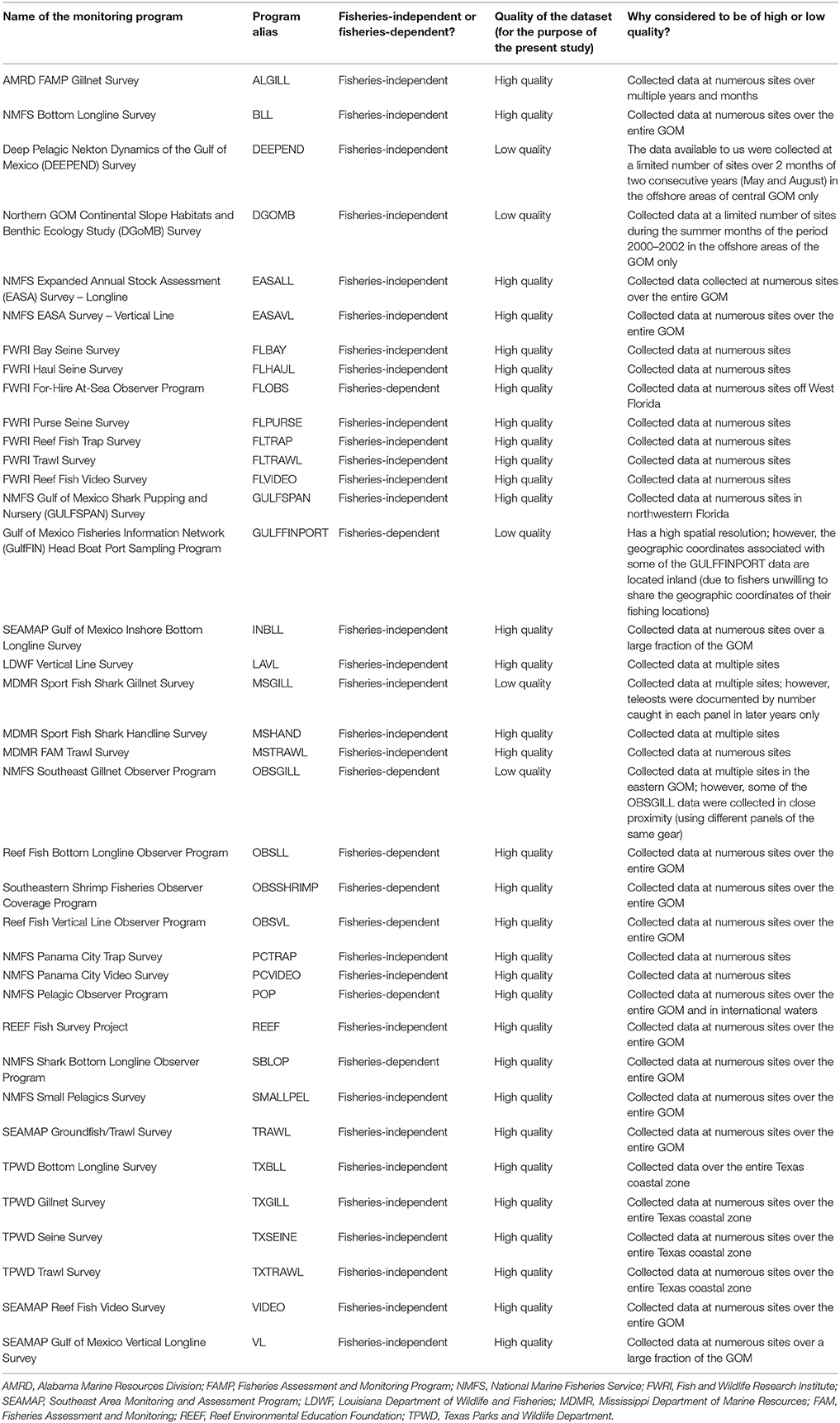
Table 2. Monitoring programs comprising the large monitoring database for the U.S. Gulf of Mexico (GOM).

A literature review was conducted to determine: (1) whether we should generate distribution maps for the juvenile and adult stages or all the life stages of the fish and invertebrate functional groups represented in Atlantis-GOM; and (2) whether or not we should generate distribution maps for different seasons for these functional groups and life stages (Supplementary Table 3). We produced distribution maps for the juvenile and adult stages of a given functional group when the literature review indicated that the functional group undertakes ontogenetic habitat shifts, i.e., changes habitats as it grows older (e.g., red grouper and gag; Mullaney, 1994; Saul et al., 2013; Carruthers et al., 2015).

Next, for each of the fish and invertebrate functional groups/life stages, we extracted the following information from each of the 37 monitoring datasets included in the large monitoring database for the U.S. GOM: (1) the longitudes and latitudes at which the sampling events occurred; (2) the years and months during which the sampling events occurred; and (3) whether, during the sampling events, the functional group/life stage considered was encountered or not (0's and 1's). To obtain encounters/non-encounters for juvenile and adult life stages, we used the body length estimates recorded by monitoring programs and body length at sexual maturity from FishBase and SeaLifeBase (Froese and Pauly, 2015; Palomares and Pauly, 2015). We gauged the quality of the 37 datasets (e.g., does the monitoring program have a high or a low spatio-temporal resolution?) as we extracted information from them (Table 2); this allowed us to identify the datasets that we should not be used when better datasets are available.

Finally, for each of the fish and invertebrate functional groups/life stages, we determined the monitoring programs from the large monitoring database for the U.S. GOM that it would be reasonable to employ to fit statistical models. To select monitoring datasets for a given functional group/life stage, we applied the following rules: (1) datasets with fewer than 50 encounters should be excluded from statistical modeling exercises (Leathwick et al., 2006; Austin, 2007; Grüss et al., 2017b,c); (2) years with fewer than five encounters should be excluded from statistical modeling exercises (Grüss et al., 2017b,c); and (3) a dataset gauged to be of low quality (for the purpose of the present study) should be excluded from statistical modeling exercises if better datasets are available (Grüss et al., 2017b).

Compilation of a Large Environmental Database for the GOM LME

A literature review was conducted to identify the environmental parameters influencing the spatial distribution patterns of the functional groups and life stages considered in this study and for which estimates could be obtained for the entire GOM LME (Supplementary Table 3). The literature review revealed that a total of 21 environmental parameters should be included in the large environmental database for the GOM LME (Table 3). Two of these 21 environmental parameters are categorical (presence/absence of seagrass, and dominant sediment type), while the others are continuous (e.g., bottom depth, SST, local percentage of mud). Some of these environmental parameters were defined for the different months of the year through the construction of “climatologies” depicting average monthly conditions for the period 2000–2016 (e.g., bottom salinity, oceanic current speed), while the others are constant over time (e.g., terrain ruggedness index, local percentage of natural reef) (Supplementary Table 4).

TABLE 3

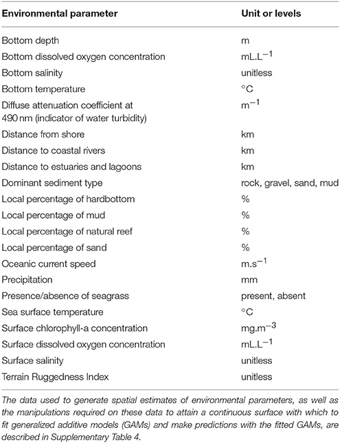
Table 3. Environmental parameters included in the large environmental database for the Gulf of Mexico Large Marine Ecosystem.

From the large environmental database for the GOM LME, we constructed a 20 × 20 km gridded map of environmental parameters covering the entire spatial domain of the Atlantis-GOM ecosystem model. This gridded map was used both for fitting binomial GAMs and making predictions with fitted binomial GAMs. To fit GAMs, the gridded map of environmental parameters was overlaid with the starting points of observations from the large monitoring database (i.e., the locations where monitoring events such as trawls where initiated). To be able to map spatial distributions using the predictions made by fitted GAMs, the gridded map of environmental parameters was overlaid with prediction grids (The construction of prediction grids for the different functional groups/life stages is described below).

Development and Evaluation of Binomial GAMs

Collinearity Analysis

Prior to fitting binomial GAMs, for each functional group/life stage, we assessed the degree of collinearity between all environmental covariates (e.g., bottom depth, SST, surface salinity, and oceanic current speed in the case of white marlin (Tetrapturus albidus; Supplementary Table 3). This collinearity analysis was needed, since statistical regressions may be sensitive to correlated covariates (Guisan et al., 2002; Dormann et al., 2013). For each functional group/life stage, we computed Pearson's correlation coefficients between environmental covariates (Booth et al., 1994; Brotons et al., 2004; Dormann et al., 2013). According to Leathwick et al. (2006) and Dormann et al. (2013), environmental covariates for which pairwise correlations exceed 0.7 in absolute value should be discarded.

Fitting of Binomial GAMs

For each of the functional groups/life stages, we fitted a binomial GAM using appropriate datasets from the large monitoring database for the U.S. GOM and the R package “mgcv” (Wood and Augustin, 2002; Wood, 2006), following the equation:

$\begin{array}{l}g(\eta )=s(x_1)+s(x_2)+\dots +s(x_n)+factor(year)\\ +factor(monitoringprogram)& (1)\end{array}$

where η is the encounter probability; g is the logit link function between η and each additive covariate; s is a thin plate regression spline fitted to a given environmental covariate; x₁, x₂, …, x_n are the environmental covariates selected after the collinearity analysis; and year and monitoring program are “nuisance variables” (i.e., variables that are not of immediate interest but that must be accounted for in the analysis) treated as fixed effect factors (Farmer and Karnauskas, 2013; Grüss et al., 2016a, 2017a). The fact that year and monitoring program are fixed effect factors entails that it will be necessary to choose a given year and a given monitoring program to make predictions with fitted GAMs (in this case, the average year effect and the monitoring program effect with the highest selectivity; Punt et al., 2000; Maunder and Punt, 2004; Farmer and Karnauskas, 2013; Grüss et al., 2016a; see subsection Production of Distribution Maps for the GOM LME from the Predictions Made by Fitted Binomial GAMs). Ecosystem models such as Atlantis-GOM require long-term averages as input (Grüss et al., 2016a; O'Farrell et al., 2017), so encounter probability predictions for an average year is a desired output of the GAMs. However, to avoid having to make predictions using the monitoring program effect with the highest selectivity, we could have developed generalized additive mixed models (GAMMs; Lin and Zhang, 1999) treating gear as a random effect rather than GAMs. We did not choose this option, because GAMMs are computationally intensive and are likely to face convergence issues when fitted to very large monitoring datasets like ours. However, Grüss et al. (2017a) showed that the spatial patterns of probability of encounter predicted by GAMs treating monitoring program as a fixed effect factor are unaffected by the monitoring program factor, and that the gross magnitude of the probabilities of encounter predicted by these GAMs are only slightly affected by the monitoring program factor.

We employed thin-plate regression splines with shrinkage, and each thin-plate regression spline was limited to four degrees of freedom (Roberts et al., 2016; Mannocci et al., 2017). For selecting environmental variables for each GAM, we used a shrinkage approach (Roberts et al., 2016; Mannocci et al., 2017). In addition to the shrinkage approach, we applied an extra penalty to each environmental covariate as the smoothing parameter approached zero, which allowed its removal when the smoothing parameter was equal to zero (Marra and Wood, 2011; Drexler and Ainsworth, 2013; Grüss et al., 2014). Once a GAM was fitted, if an environmental covariate p-value had a p > 0.05, it was removed and the model was refitted (Koubbi et al., 2006; Weber and McClatchie, 2010; Grüss et al., 2014, 2016d, 2017a; Chagaris et al., 2015). The restricted maximum likelihood (REML) optimization method was employed (Wood, 2011).

The data from the large monitoring database, like any ecological data, are likely to show spatial structure (Legendre, 1993; Guisan and Thuiller, 2005; Dormann et al., 2007; Elith and Leathwick, 2009). To examine this issue, we constructed empirical variograms of the residuals from the GAMs (Supplementary Data Sheet 1). Spatial structure is absent when an empirical variogram is largely flat, while an empirical variogram with patterns indicates that there is spatial autocorrelation in model residuals (Cressie, 1993). Empirical variograms tend to have a roughly logarithmic form in ecological data. The existence of spatial autocorrelation can also be revealed by spatial clusters of positive and negative residuals (Cressie, 1993; Grüss et al., 2016d).

Evaluation of Binomial GAMs

To evaluate the validity of the fitted GAMs, we used the “Leave Group Out Cross Validation” procedure (Hastie et al., 2001; Kuhn and Johnson, 2013). In this iterative cross-validation procedure, for each functional group/life stage, monitoring data were randomly split into training and test datasets, with 60% of the data going to the training dataset and the rest of the data to the test dataset (Grüss et al., 2016d). We fitted binomial GAMs to the training dataset employing the fitting procedure described in subsection Fitting of Binomial GAMs, and then evaluated the GAMs using the test dataset. We repeated this process 10 times, i.e., for each individual binomial GAM, 10 models were fitted to training datasets and then evaluated using the test datasets corresponding to the training datasets.

Two metrics were utilized to evaluate binomial GAMs through the Leave Group Out Cross Validation procedure: (1) the area under the receiver operating characteristic (ROC) curve (AUC), which reflects if binomial GAMs are able to discriminate between encounters and non-encounters (Hanley and McNeil, 1982); and (2) the adjusted coefficient of determination (adjusted R²), which is a means to measure the proportion of variance of the encounter probability explained by binomial GAMs (Legendre and Legendre, 1998). An AUC value of 0.5 indicates no improvement in predictability over random chance, while an AUC value of 1 is indicative of perfect discrimination between encounters and non-encounters (Swets, 1988; Fielding and Bell, 1997; Pearce and Ferrier, 2000; Wintle et al., 2005; Leathwick et al., 2006; Heinänen et al., 2008). The R package “pROC” was employed to construct ROC curves and compute AUCs (Robin et al., 2011).

For each functional group/life stage, a binomial GAM passed the validation test if: (1) the median AUC value estimated via the Leave Group Out Cross Validation procedure was larger than 0.7 (Hanley and McNeil, 1982; Swets, 1988; Pearce and Ferrier, 2000); and (2) the median adjusted R² estimated via the Leave Group Out Cross Validation procedure was larger than 0.1 (Legendre and Legendre, 1998).

Production of Distribution Maps for the GOM LME from the Predictions Made by Fitted Binomial GAMs

After all binomial GAMs were fitted and validated, we employed them to predict the long-term probability of encounter of functional groups and life stages in the GOM LME, at different seasons. To be able to generate long-term probability of encounter maps, we constructed 20 × 20 km prediction grids for the GOM LME, based on the depth ranges at which the functional groups/life stages are encountered by the monitoring programs of the large monitoring database for the U.S. GOM. To determine the depth at which the functional groups/life stages are encountered by monitoring programs, we used the SRTM30 PLUS global bathymetry grid to generate a depth raster with a resolution of 20 km; we obtained the SRTM30 PLUS global bathymetry grid from the Gulf of Mexico Coastal Observing System² We made predictions with fitted binomial GAMs, using the 20 × 20 km prediction grids, the 20 × 20 km gridded map of environmental parameters, and the average year effect and the monitoring program effect with the highest selectivity (Punt et al., 2000; Maunder and Punt, 2004; Farmer and Karnauskas, 2013; Grüss et al., 2016a).

Development and Evaluation of Geostatistical Binomial Glmms

Fitting of Geostatistical Binomial GLMMs

Our geostatistical modeling approach is described only briefly below; the reader is referred to Grüss et al. (2017b,c) for details, since we applied the same methodology as theirs.

The geostatistical models employed here are spatio-temporal binomial GLMMs which predict encounter probabilities, and Gaussian Markov random fields are used to model spatial residuals in encounter probability (Grüss et al., 2017b,c). We approximated Gaussian Markov random fields using 1,000 “knots”, for computational efficiency (Thorson et al., 2015); for each functional group/life stage/season, the location of the knots was determined through the application of a k-means algorithm to the locations of the data of the large monitoring database for the U.S. GOM, which distributes knots over space after having considered the sampling intensity of the different monitoring programs retained for a given functional group/life stage/season.

We fitted our geostatistical binomial GLMMs to the large monitoring database for the U.S. GOM following the equation:

$\begin{array}{ll}g(p_i)={\displaystyle \sum _{t=1}^{n_t}}{\beta }_t{Y}_{i,t}+{\displaystyle \sum _{m=1}^{n_m}}{\gamma }_m{G}_{i,m}+{\epsilon }_{J(i)}& (2)\end{array}$

where p_i is the encounter probability at site s(i); g is the logit link function between p_i and each term provided at the right side of the equation; ε_J(i) are the effects of the spatial residuals in encounter probability at J(i), the nearest knot to sample i, on the logit scale (random effects); ${\sum }_{m=1}^{n_m}{\gamma }_m{G}_{i,m}$ is the effect of monitoring program on p_i on the logit scale; and ${\sum }_{t=1}^{n_t}{\beta }_t{Y}_{i,t}$ is the effect of year on p_i on the logit scale. The effect of monitoring program is treated as random via the implementation of REML, and the year effect is fixed.

With regards to the effect of monitoring program, G_i,m is a design matrix such that G_i,m is 1 for the monitoring program m which collected sample i and 0 otherwise; γ_m is a monitoring program effect (where γ_m = 0 for the monitoring program m with the largest sample size for a given functional group/life stage/season; we imposed this constraint for identifiability of all year effects β_t); and n_m is the number of monitoring programs retained for the functional group/life stage/season considered.

With regards to the effect of year, Y_i,t is a design matrix such that Y_i,t is 1 for the year t during which sample i was collected and 0 otherwise; β_t is an intercept varying among years; and n_t is the number of sampling years for the functional group/life stage/season considered. Our geostatistical GLMMs use data in every year t to predict what would arise in any site i. The intercept β_t then means that encounter probability is scaled up or down amongst years, where the change in encounter probability (in logit-odds) is the same between any 2 years for any site. Therefore, the intercept β_t accounts for the fact that different years might have a higher or lower encounter probability for all sites in a given year. If the spatial footprint of a given monitoring program changes amongst years, then our geostatistical GLMMs account for this by comparing it with the predicted encounter probability at each site. If the data for a given site and monitoring program is higher than the prediction for that site, this leverage causes our geostatistical GLMMs to increase the predicted encounter probability at that site (in order to decrease model residuals).

Finally, with regards to the random effects ε_J(i), those follow a multivariate normal distribution:

$\begin{array}{ll}\epsilon ~MN(0,\Sigma )& (3)\end{array}$

where MN is the multivariate normal distribution, whose expected value was fixed to 0 for each site; and Σ is a covariance matrix for ε at each site. We assumed that the covariance between sites s and s′ is stationary and follows a Matérn distribution with smoothness ν = 1:

$\begin{array}{ll}\Sigma (s,{s^{\prime }}^{})={\sigma }_{\epsilon }^2.Matérn(||\text{H}(s-s^{\prime })||;\kappa )& (4)\end{array}$

where σ_ε is the standard deviation of ε; H is the linear transformation representing geometric anisotropy³; (s − s′) = (x − x′, y − y′) is the difference in eastings and northings between sites s and s′; H(s − s′) is the distance between sites after having accounted for geometric anisotropy (Cressie and Wikle, 2015; Thorson et al., 2015); and κ is the range parameter, which governs the distance over which covariance reaches 10% of its pointwise value (Thorson et al., 2016).

To estimate the fixed effect of year, we employed maximum marginal likelihood while integrating across the random effects of gear and ε; the Laplace approximation implemented in the Template Model Builder (Kristensen et al., 2016) was used to approximate maximum marginal likelihood. More precisely, we first approximated the probability of the random effects through use of the stochastic partial differential equation approximation for Gaussian random fields with geometric anisotropy described in Thorson et al. (2015) and based on methods in Lindgren et al. (2011). Then, we maximized the marginal likelihood through conventional non-linear optimization in the R environment (R Core Development Team, 2013).

Evaluation of Geostatistical Binomial GLMMs

To determine whether the geostatistical binomial GLMMs fitted for the different functional groups/life stages/seasons converged, we examined whether any of the parameters H, κ and σ_ε hit an upper or lower bound, and whether the absolute value of the final gradient for each of these parameters was close to zero. Moreover, to gauge geostatistical GLMM fits, we calculated Pearson residuals for the samples considered for each functional group/life stage/season, as described in Supplementary Data Sheet 2.

Production of Distribution Maps for the U.S. GOM from the Predictions Made by Fitted Geostatistical Binomial GLMMs

To be able to generate probability of encounter maps from predictions made by geostatistical binomial GLMMs, we first constructed 20 × 20 km prediction grids for each functional group/life stage/season. To do so, we generated a 20 × 20 km spatial grid covering the entire U.S. GOM (Figure 3). Then, we employed the depth raster we produced from the SRTM30 PLUS global bathymetry grid (see subsection Production of Distribution Maps for the GOM LME from the Predictions Made by Fitted Binomial GAMs) to determine the depths at which each of the study functional groups/life stages are encountered by monitoring programs year-round or at different seasons, Finally, we defined prediction grids for each functional group/life stage/season from the spatial grid for the U.S. GOM (Figure 3), based on the ranges of longitude, latitude and depth at which the functional groups/life stages are encountered by monitoring programs year-round or at different seasons.

FIGURE 3

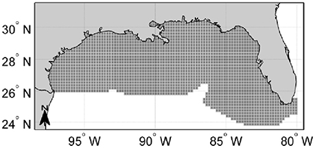
Figure 3. Spatial grid (20 × 20 km) for the U.S. Gulf of Mexico.

To generate the distribution maps for the U.S. GOM for each of the functional groups/life stages/seasons, we made the assumption that the Gaussian random field in each cell of their prediction grid is equal to the value of the Gaussian random field at the nearest knot. First, for each functional group/life stage/season, we used the fitted geostatistical binomial GLMM for that functional group/life stage/season to produce a probability of encounter map for each of the sampling years. Then, the probability of encounter maps for each sampling year were averaged to construct one final, long-term probability of encounter map for each functional group/life stage/season for the U.S. GOM.

Construction of Distribution Maps Usable in the Atlantis-GOM Ecosystem Model

To construct a distribution map for each functional group/life stage/season that is usable in the Atlantis-GOM ecosystem model, we proceeded in three steps (Steps 4A,B, 5A,B, and 6 in Figure 2).

First, we generated a map of relative abundance for the GOM LME from the long-term probability of encounter map produced from GAM predictions (see subsection Production of Distribution Maps for the GOM LME from the Predictions Made by Fitted Binomial GAMs), such that the sum of relative abundances for the map is equal to 1.0 (Step 4A in Figure 2). This resulted in a map such that the sum of relative abundances in the U.S. GOM is equal to N1 and the sum of relative abundances in the southern GOM is equal to N2, such that N1 + N2 = 1.0. In parallel, we generated a map of relative abundance for the U.S. GOM from the long-term probability of encounter map produced from geostatistical GLMM predictions (see subsection Production of Distribution Maps for the U.S. GOM from the Predictions Made by Fitted Geostatistical Binomial GLMMs), such that the sum of relative abundances for the map is equal to 1.0 (Step 4B in Figure 2).

Second, we generated a map a relative abundance for the southern GOM from the map of relative abundance for the GOM LME (Step 5A in Figure 2), such that the sum of relative abundances for the map is equal to N2. In parallel, we generated a map of relative abundance for the U.S. GOM (Step 5B in Figure 2), which reflects the spatial patterns of relative abundance of the map produced in Step 4B while accounting for relative abundance in the U.S. GOM relative to the southern GOM according to the map produced in Step 4A (such that the sum of relative abundances for the map produced in Step 5B is equal to N1).

Third, we combined the map of relative abundance for the southern GOM produced in Step 5A and the map of relative abundance for the U.S. GOM produced in Step 5B, to obtain a map of relative abundance usable in the Atlantis-GOM model (Step 6 in Figure 2).

In the following, for illustration purposes, we analyze in detail the distribution maps we generated for Atlantis-GOM for the following three life stages: juvenile pink shrimp (Farfantepenaeus duorarum), adult pink shrimp, and adult red grouper. We also compare the distribution maps for Atlantis-GOM produced in this study to those produced in Drexler and Ainsworth (2013). For all the fish and invertebrates represented in Atlantis-GOM, Drexler and Ainsworth (2013) fitted negative binomial GAMs integrating dominant sediment type, bottom depth, bottom temperature, bottom DO concentration and surface chlorophyll-a concentration to abundance data from the SEAMAP (Southeast Area Monitoring and Assessment Program) Groundfish/Trawl Survey; the authors then employed GAM predictions to construct maps of relative abundance usable in Atlantis-GOM.

Results

Development and Evaluation of Binomial GAMs

Fitting of Binomial GAMs

It was possible to use the encounter/non-encounter data of the large monitoring database for the U.S. GOM to fit reasonable binomial GAMs for the majority of the fish and invertebrate functional groups and life stages represented in Atlantis-GOM (Supplementary Table 3). Some of the binomial GAMs we initially fitted did not pass the validation test, because their median adjusted R² (produced through the Leave Group Out Cross Validation procedure) was smaller than 0.1; therefore, we decided not to employ these GAMs but rather GAMs for related functional groups/life stages to generate distribution maps (Supplementary Table 3). For instance, we decided to use: (1) a GAM fitted for all life stages of ladyfish (Elops saurus) instead of the GAMs fitted for the juvenile and adult stages of that species to produce distribution maps; and (2) the GAM of white marlin to produce distribution maps for blue marlin (Makaira nigricans). Moreover, none of the datasets included in the large monitoring database for the U.S. GOM provided encounter/non-encounter data for filter feeding sharks; therefore, we were unable to fit binomial models for this functional group. Ultimately, we fitted a total of 76 GAMs in the present study (Supplementary Table 3).

Evaluation of Binomial GAMs

We computed adjusted R²'s and AUCs for the 76 binomial GAMs we fitted using the Leave Group Out Cross Validation procedure (Supplementary Table 5) and, for each of these GAMs, we constructed empirical variograms of the residuals (Supplementary Figure 1).

Fifty five of the 76 fitted binomial GAMs (i.e., 72% of the fitted GAMs) had a median AUC value in the range of 0.7–0.9 (Supplementary Table 5). The 21 other fitted binomial GAMs had a median AUC value larger than 0.9. Bluefin tuna (Thunnus thynnus) had the lowest median AUC (0.708), while yellowfin tuna (Thunnus albacares) had the highest (0.986).

The median adjusted R²'s produced through the Leave Group Out Cross Validation procedure ranged between 0.10 (adult gag, bluefin tuna, and adult pink shrimp) and 0.84 (yellowfin tuna) (Supplementary Table 5). Fifty eight of the 76 fitted binomial GAMs had a median adjusted R² value in the range of 0.1–0.3. Only three binomial GAMs had a median adjusted R² at or >0.5 [those fitted for juvenile black drum (Pogonias cromis), yellowfin tuna, and squids].

The empirical variograms show that, in the great majority of cases, GAM residuals are spatially autocorrelated (Supplementary Figure 1). Exceptions to this pattern include juvenile red drum (Sciaenops ocellatus), juvenile sheepshead (Archosargus probatocephalus), juvenile snooks (Centropomus spp.), adult snooks, and adult stone crab (Menippe mercenaria). When the residuals from a fitted binomial GAM showed spatial structure, this spatial structure was generally significant.

Development and Evaluation of Geostatistical Binomial GLMMs

Fitting of Geostatistical Binomial GLMMs

It was not possible to fit geostatistical binomial GLMMs for all the fish and invertebrate functional groups and life stages for which we fitted binomial GAMs (Table 4 and Supplementary Table 6). The reasons for this included: (1) an absence of monitoring data for Louisiana and Mississippi waters in the large monitoring database (e.g., juvenile and adult black drums, ladyfish, mullets); (2) and absence of monitoring data for Louisiana, Mississippi and Alabama waters in the large monitoring database (e.g., juvenile and adult sheepshead, oysters); or (3) monitoring data not covering the full depth range of the functional group/life stage under consideration (e.g., bluefin tuna, white marlin) (Table 4). Ultimately, we fitted a total of 77 geostatistical binomial GLMMs (Supplementary Table 6).

TABLE 4

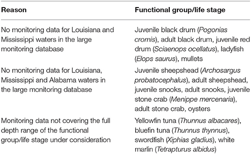
Table 4. Functional groups and life stages for which it was not possible to develop geostatistical binomial generalized linear mixed models in the present study.

Evaluation of Geostatistical Binomial GLMMs

For all the functional groups/life stages/seasons, we found that none of the parameters H, κ and σ_ε hit an upper or lower bound, and that the absolute value of the final gradient for each of these parameters was smaller than 0.002 (Supplementary Table 7). Thus, there was no evidence of non-convergence for any of the functional groups, life stages and seasons.

For all the functional groups/life stages/seasons, observed encounter frequencies for either low or high probability samples were generally within or extremely close to the 95% confidence interval for predicted probability of encounter (Supplementary Figure 2). Exceptions to this general pattern occurred for: (1) juvenile gag; (2) juvenile shallow Serranidae; (3) vermilion snapper (Rhomboplites aurorubens); (4) juvenile large reef fish; (5) adult large reef fish; (6) Spanish sardine (Sardinella aurita); (7) juvenile menhadens (Brevoortia spp.) in fall-winter; (8) adult menhadens in spring-summer; and (9) carnivorous macrobenthos. In the nine above mentioned cases, observed encounter frequency for the highest probability samples were noticeably smaller than the 95% confidence interval for predicted probability of encounter (Supplementary Figure 2). Yet, in these nine cases, geostatistical binomial GLMMs did not systematically overestimate or underestimate encounter probability in any area of the U.S. GOM (Supplementary Figure 3).

Distribution Maps for the Atlantis-GOM Ecosystem Model

From the large monitoring database, we were able to construct a total of 53 annual maps and 64 seasonal maps (for 32 different fish and invertebrate functional groups/life stages) for Atlantis-GOM. We were unable to strictly follow the methodology depicted in Figure 2 for the functional groups and life stages for which it was not possible to fit geostatistical binomial GLMMs; for those, we produced distribution maps for Atlantis-GOM directly from GAM predictions. Here, we present a few of the distribution maps we constructed (Figure 4); the rest of the distribution maps are provided in Supplementary Figure 4.

FIGURE 4

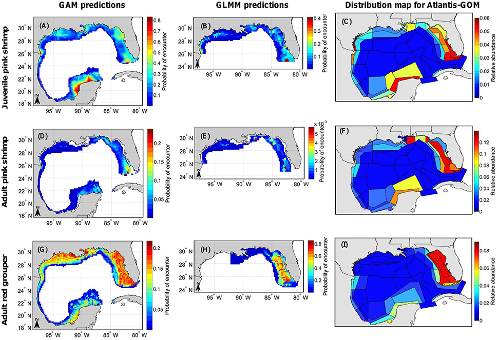
Figure 4. Distribution maps produced for (A–C) juvenile pink shrimp (Farfantepenaeus duorarum), (D–F) adult pink shrimp, and (G–I) adult red grouper (Epinephelus morio). (A,D,G) are probability of encounter maps for the entire Gulf of Mexico Large Marine Ecosystem generated from the predictions of generalized additive models (GAMs). (B,E,H) are probability of encounter maps for the U.S. Gulf of Mexico generated from the predictions of geostatistical generalized linear mixed models (GLMMs). Finally, (C,F,I) are maps of relative abundance usable in the Atlantis-GOM ecosystem model (such that the sum of relative abundances for each map is equal to 1.0).

GAM and GLMM predictions were combined to generate annual distribution maps for the juvenile and adult stages of pink shrimp (Figures 4A–F). Both the binomial GAM and the geostatistical binomial GLMM fitted for juvenile pink shrimp predicted the life stage to be primarily encountered from Apalachicola (Florida) to the southern West Florida Shelf at depths < 40 m, especially in the area around the Dry Tortugas, as well as on the Texas-Mexico border (Figures 4A,B). The binomial GAM of juvenile pink shrimp also predicted the life stage to be encountered all over the Campeche Bank, mainly at depths < 40 m (Figure 4B). Both the binomial GAM and the geostatistical binomial GLMM fitted for adult pink shrimp predicted the life stage to primarily occur from Apalachicola to the southern West Florida Shelf at depths ranging between 20 and 80 m, particularly in the area around the Florida Keys and the Dry Tortugas, as well as in the region off Alabama and Mississippi where depth ranges between 20 and 40 m and on the Texas-Mexico border (Figures 4D,E). Yet, contrary to the binomial GAM, the geostatistical binomial GLMM fitted for adult pink shrimp predicted similar probabilities of encounter in the area around the Florida Keys and the Dry Tortugas and in the region off Alabama and Mississippi where depth ranges between 20 and 40 m. The binomial GAM of adult pink shrimp also predicted that the northern Campeche Bank is a hotspot of probability of encounter for adult pink shrimp (Figure 4E).

GAM and GLMM predictions were also combined to produce an annual distribution map for adult red grouper (Figures 4G–I). The binomial GAM of adult red grouper predicted the life stage to be mainly encountered over the entire U.S. GOM shelf at depths less than 60 m (Figure 4G). By contrast, the geostatistical binomial GLMM of adult red grouper predicted the life stage to be encountered primarily from Apalachicola to the southern West Florida Shelf at depths < 60 m, to be very rarely encountered in Alabama, Mississippi and Louisiana waters, and to be absent from Texas waters (Figure 4H). The absence of adult red grouper from Texas waters is due to the fact that none of the monitoring programs included in the large monitoring database for the U.S. GOM encountered adult red grouper in Texas waters, although there was a large sample size of observations using gears that captured red groupers in other regions of the U.S. GOM. Consequently, the probability of encounter map produced from geostatistical GLMM predictions did not include Texas waters, and, in the map of relative abundance produced for Atlantis-GOM, adult red grouper is assumed to be absent from Texas waters (Figure 4I). The relative abundance of adult red grouper in the southern GOM was determined from the probability of encounter map produced from GAM predictions; in the southern GOM, the bulk of adult red groupers were predicted to be encountered all over the Campeche Bank, mainly at depths < 60 m (Figures 4G,I).

Differences between the distribution maps for Atlantis-GOM produced in this study and those produced in Drexler and Ainsworth (2013) are more or less pronounced depending on the functional group/life stage under consideration (Figure 5). Contrary to the present study, Drexler and Ainsworth (2013) produced one single map for pink shrimp (i.e., for juveniles and adults combined). Pink shrimp is more homogeneously distributed in the GOM LME according to Drexler and Ainsworth's (2013) approach than according to our methodology (Figures 5A,B vs. Figures 5C,D). In particular, Drexler and Ainsworth's (2013) approach predicts pink shrimp to be relatively abundant over the shelves of central and eastern Texas and Louisiana, contrary to our methodology. The differences between the spatial distributions predicted in Drexler and Ainsworth (2013) and those predicted in this study are more pronounced for adult red grouper (Figure 5E vs. Figure 5F). Importantly, Drexler and Ainsworth (2013) predicted adult red grouper to be relatively abundant on the Texas shelf, while adult red grouper is absent from this area according to the map of relative abundance we generated for Atlantis-GOM in the present study.

FIGURE 5

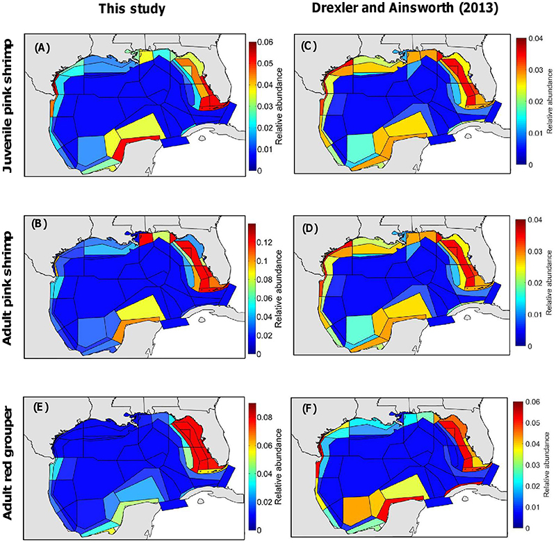
Figure 5. Maps of relative abundance for the Atlantis-GOM ecosystem model (such that the sum of relative abundances for each map is equal to 1.0), produced (A–C,E) in the present study and (C,D,F) in Drexler and Ainsworth (2013). (A,C) are for juvenile pink shrimp (Farfantepenaeus duorarum), (B,D) are for adult pink shrimp, and (E,F) are for adult red grouper (Epinephelus morio).

Discussion

In the present study, we developed a novel methodology for producing distribution maps for a spatially-explicit ecosystem model using large monitoring and environmental databases and a combination of interpolation and extrapolation. This novel methodology has a number of advantages. First, it makes use of all the monitoring data collected in the ecosystem of interest using random sampling schemes, thereby allowing the development of more reliable statistical models. Then, our methodology performs extrapolation using GAMs integrating only environmental covariates that are pertinent for the functional groups and life stages of interest. Finally, our methodology performs interpolation using geostatistical models in the regions where monitoring data are available, thereby accounting for spatial structure in spatial distribution patterns in those regions. This is particularly desirable because the residuals from GAMs fitted to monitoring data typically show spatial structure (as was the case in the present study; Supplementary Figure 1).

In order to construct reliable distribution maps for the Atlantis-GOM ecosystem model, we decided not to strictly follow our methodology in some cases. First, when a GAM did not pass the validation test, we used a GAM for a related functional group/life stage to generate distribution maps for the GOM LME. Second, we did not fit geostatistical GLMMs for those functional groups and life stages whose depth, longitudinal and latitudinal ranges are not entirely covered by the monitoring data from the large monitoring database for the U.S. GOM. For those, only GAM predictions were employed to obtain distribution maps for Atlantis-GOM. From the large monitoring and environmental databases, we were able to produce 53 annual maps and 64 seasonal maps (for 32 different functional groups/life stages) for the Atlantis-GOM model. We had no data for filter feeding sharks [basking shark (Cetorhinus maximus), and whale shark (Rhincodon typus)] in the large monitoring database for the U.S. GOM. To be able to generate a distribution map for this functional group, we fitted a MaxEnt model (Phillips et al., 2006, 2017) to presence-only data for basking and whale sharks obtained from the Ocean Biogeographic Information System⁴ (Supplementary Data Sheet 3). Thus, ultimately, we produced a total of 117 annual and seasonal maps for the fish and invertebrate functional groups and life stages represented in the Atlantis-GOM ecosystem model (Supplementary Figure 4).

The usefulness of our methodology combining GAM and geostatistical GLMM predictions is exemplified by the distribution maps generated for pink shrimp and adult red grouper (Figure 4). The distribution maps produced for juvenile and adult pink shrimps from GAM and geostatistical GLMM predictions concurred with previous studies in that pink shrimp hotspots are found on the West Florida Shelf, around the Dry Tortugas and the Florida Keys, in the region off Alabama and Mississippi where depth ranges between 20 and 40 m, on the Texas-Mexico border, and on the Campeche Bank (Costello and Allen, 1970; Bielsa et al., 1983; Ramirez-Rodriguez et al., 2003; Drexler and Ainsworth, 2013; Grüss et al., 2014). However, reflecting monitoring data for the U.S. GOM, the geostatistical GLMM of adult pink shrimp predicted that the life stage has a very high probability to be encountered in the region off Alabama and Mississippi where depth ranges between 20 and 40 m, contrary to the GAM of adult pink shrimp. More importantly, the GAM of adult red grouper was unable to correctly predict the spatial distribution of the life stage in the U.S. GOM. Consistent with the literature (Coleman et al., 1996, 2011; Lombardi-Carlson et al., 2008; Albañez-Lucero and Arreguin-Sanchez, 2009), the GAM and the geostatistical GLMM of adult red grouper predicted that the life stage has a high probability to be encountered over the entire West Florida and on the Campeche Bank. However, like the GAM fitted in Drexler and Ainsworth (2013), the GAM of adult red grouper fitted in this study also wrongly predicted that the life stage has a high probability to be encountered over the rest of the U.S. GOM shelf, while there is a consensus in the literature that adult red grouper is very rarely encountered west of the Florida-Alabama border (Coleman et al., 1996, 2011; Franks, 2005; Burns and Robbins, 2006; Lombardi-Carlson et al., 2008); it has been suggested that the presence of red grouper west of the Florida-Alabama border relates to displacement of individuals by storms and hurricanes or anomalous oceanic current patterns resulting in the settlement of grouper larvae west of the De Soto Canyon (Franks, 2005; Burns and Robbins, 2006; Dance et al., 2011; Karnauskas et al., 2013).

A major limitation of the methodology introduced in this study is that it relies on GAMs that do not account for spatial structure. One can account for spatial structure in GAMs through the integration of a spatial autocorrelation term (Guisan and Thuiller, 2005; Zuur et al., 2014), or of an interaction term between eastings and northings (Wood, 2006; Grüss et al., 2016d); however, it was not possible to implement either of these options in the present study, since we needed to perform extrapolation to the entire GOM LME while we had monitoring data only for the U.S. GOM. The autocorrelated residual variance found for the great majority of the functional groups/life stages in this study (Supplementary Figure 1), combined with the broad spatial scale of the maps of probability of encounter we generated, mean that these maps are not particularly useful for localized predictions. By necessity, mapping the general spatial distribution of functional groups/life stages usually requires some abstraction of the populations. Hence, the predictions we made with GAMs in the present study would not be useful for informing whether one would be likely to capture functional groups/life stages at a particular location of the GOM LME. This is evident, for example, if we compare the ranges of autocorrelation between the residuals of the model fits for gag and red grouper life stages found in this study (Supplementary Figure 1) with the smaller ones found when modeling individual catch per unit effort information in Saul et al. (2013); the ranges of autocorrelation for gag and red grouper found in Saul et al. (2013) were much closer to the sizes of individual habitat patches. Thus, it is important to emphasize that the modeled products that we reported in this study are valuable to capture larger spatial patterns necessary for running simulations with ecosystem models, but not to predict the spatial distribution patterns of fish and invertebrate populations with high precision.

Another limitation of the present study is that, for each functional group, we relied on one reference species to determine whether to model ontogenetic differences in spatial distribution patterns and environmental influences on spatial distribution patterns (Supplementary Table 3). In other words, we made the assumption that all the species of a given functional group share the same spatial distribution patterns, namely those of the reference species of the functional group (although data extraction and statistical model fitting considered all the species making up the study functional groups). This assumption is reasonable given the large number of fish and invertebrates we had to deal with (63) and the very low spatial resolution of the Atlantis-GOM ecosystem model (Figure 1B). Yet, studies using our methodology to construct distribution maps for a spatially-explicit ecosystem model with the higher resolution than that of Atlantis-GOM may want to proceed another way; for example, these studies may want to rely on several reference species for deciding whether the spatial distribution patterns of the juveniles and adults of each functional group differ and which environmental parameters should be integrated in the GAM of each functional group.

Some modifications could be introduced in the structure and validation process of our geostatistical models in future studies. For simplicity, we did not integrate environmental parameters in our geostatistical GLMMs, because preliminary analyses conducted for previous studies using geostatistical models to infer fish and invertebrate spatial distributions in the U.S. GOM found that spatial residuals in probability of encounter have a much larger influence on probabilities of encounter than environmental variables (Grüss et al., 2017b,c). Also, typically, relationships between the probability of encounter of fish and invertebrates and environmental parameters are non-linear, which is something that the geostatistical GLMMs employed in this study cannot represent at present. Thus, it appeared more appropriate not to integrate environmental parameters in our geostatistical models, and we recommend that the future studies wishing to integrate environmental parameters in our geostatistical models should first incorporate non-linearities into these models. Moreover, to validate our geostatistical models, we used standard procedures, i.e., convergence diagnostics and analyses of Pearson residuals (Thorson et al., 2015; Grüss et al., 2017b,c). Future studies could implement the Leave Group Out Cross Validation procedure for our geostatistical models and estimate their adjusted R² and AUC; it would then be possible to compare the AUCs of binomial GAMs with those of binomial geostatistical GLMMs fitted to the same monitoring data and, thus, to compare the ability of binomial GAMs and binomial geostatistical GLMMs to discriminate between encounters and non-encounters.

We generated maps of relative abundance for the Atlantis-GOM ecosystem model from probability of encounter maps. Thus, as is often done in the mapping literature (e.g., Maxwell et al., 2009; Hattab et al., 2013; Cormon et al., 2014; Grüss et al., 2014, 2017b,c), we assumed a linear relationship between probability of encounter and abundance. This assumption is appropriate for many of the functional groups represented in Atlantis-GOM that are structure-oriented; the abundance of structure-oriented functional groups, such as red grouper and gag, may be primarily determined by the encounter/non-encounter of a suitable structure (Saul et al., 2013; Grüss et al., 2017c). Yet, spatial patterns of probability of encounter and spatial patterns of abundance often rely on slightly different determinants (Nielsen et al., 2005; Koubbi et al., 2006; Aarts et al., 2012; Grüss et al., 2014); thus, if we had produced distribution maps from abundance predictions (e.g., if we had had monitoring data for the entire GOM LME), some of those distribution maps may have been slightly different from the distribution maps constructed in the present study. In the future, if we had access to a reasonable amount of monitoring data for the southern GOM, it would be interesting to evaluate the consequences of employing abundance vs. probability of encounter maps to produce maps of relative abundance for Atlantis-GOM with our methodology.

The goal of this study was to obtain the maximum of data possible to generate distribution maps for a spatially-explicit ecosystem model. However, while our methodology represents a an improvement over previous ones (Grüss et al., 2016a), further improvements could be made. First, for the sake of statistical rigor, only monitoring data collected using random sampling schemes were employed to fit statistical models in the present study. Developing methods to use data from both random and fixed sampling stations would allow us to fit geostatistical models for coastal functional groups/life stages such as juvenile red drum and juvenile and adult snooks (Table 4) for which a large amount of monitoring data is collected using fixed sampling schemes in Louisiana, Mississippi and Alabama (Grüss et al., 2016a). Moreover, rather than combining interpolation and extrapolation as we did, future studies could employ only interpolation and combine the predictions made by different geostatistical models, each fitted to the monitoring data collected in a given region (e.g., in the waters of the different countries bordering a LME). Such an endeavor would be highly challenging in our case, due to the scarcity or limited access to monitoring data collected in the southern GOM.

Our inability to fit geostatistical binomial GLMMs for some of the functional groups and life stages represented in Atlantis-GOM revealed data gaps for two groups of fish and invertebrates of the U.S. GOM: (1) coastal functional groups and life stages, such as juvenile red drum, juvenile and adult snooks, ladyfish and oysters; and (2) large pelagic fish, such as bluefin tuna and white marlin (Table 4). Data collected at random stations are missing for Louisiana, Mississippi and Alabama for the first group, as mentioned above. In parallel to the development of new statistical methodologies employing monitoring data collected using fixed sampling schemes, we encourage the initiation of new monitoring programs using random sampling schemes in Louisiana, Mississippi and Alabama, for the sake of having a set of monitoring programs using similar sampling protocols over the entire U.S. GOM. Data for species such as bluefin tuna and white marlin are collected almost exclusively by the National Marine Fisheries Service Pelagic Observer Program, which operates in the offshore waters of the GOM LME, while these species are found both inshore and offshore in the GOM. We recommend the use of fisheries-independent longline surveys to collect data for these species in inshore areas of the GOM and the development of statistical models that can be fit to a mix of data collected using fixed and random samplings schemes.

The methodology developed in the present study will allow for the use of more reliable inputs in spatially-explicit ecosystem models. Spatially-explicit ecosystem models, especially highly sophisticated models such as applications of the Atlantis modeling platforms, rely on numerous data inputs, many of which can have a significant impact on ecosystem model predictions (Fulton et al., 2007; Shin et al., 2010; Walters et al., 2010; Steele et al., 2013). Many spatially-explicit ecosystem models have been designed worldwide (Fulton, 2010; Espinoza-Tenorio et al., 2012; Steele et al., 2013), and significant attention has been devoted to enhance the structure and assumptions of ecosystem modeling platforms (e.g., Shin et al., 2010; Steenbeek et al., 2013, 2016; Travers-Trolet et al., 2014; Grüss et al., 2016b,c). Therefore, it is now high time to develop and employ methodologies such as ours for ensuring that the spatially-explicit ecosystem models available around the world are provided with reliable inputs generated using the best available data and information. We hope that the methodology developed in this study will serve other regions of the world, particularly LMEs bordered by several countries (e.g., the Benguela Current LME, and the Humboldt Current LME).

Author Contributions

Designed and analyzed the models: AG, MD. Conceived the models: AG, MD, CA, and EB. Conducted the literature review: AG and JT. Queried the data: AG and ML. All authors contributed to writing the paper.

Funding

This work was funded in part by the Florida RESTORE Act Centers of Excellence Research Grants Program, Subagreement No. 2015-01-UM-522.

Conflict of Interest Statement

The authors declare that the research was conducted in the absence of any commercial or financial relationships that could be construed as a potential conflict of interest.

Acknowledgments

We wish to thank two reviewers for their insightful comments, which have improved the quality and scope of our manuscript. We would like to thank very much the following people for having provided us with data for the large monitoring database for the U.S. Gulf of Mexico: Adam G. Pollack, Alisha Gray, April Cook, Beverly Sauls, Brandi Noble, Chris Gardner, Christy Pattengill-Semmens, Doug DeVries, Elizabeth Scott-Denton, Evan John Anderson, Fernando Martinez-Andrade, Gilbert Rowe, Jeff Rester, Jill Hendon, John Carlson, John Mareska, Kelly Fitzpatrick, Kenneth Brennan, Lawrence Beerkircher, Matthew D. Campbell, Mike Brainard, Mike Harden, Nicole Smith, Rick Burris, Steve Turner, Theodore S. Switzer, Tim MacDonald, and Tracey T. Sutton. The PCTRAP, PCVIDEO, GULFSPAN, OBSLL, OBSVL, OBSSHRIMP, OBSGILL, SBLOP and POP data products were produced without the involvement of NOAA Fisheries staff, and NOAA Fisheries cannot vouch for the validity of these products. The TRAWL and INBLL data were produced without the involvement of SEAMAP partners. Therefore, SEAMAP and its partners cannot vouch for the validity of these products. The FLBAY, FLHAUL, FLOBS, FLPURSE, FLTRAP, FLTRAWL and FLVIDEO data products were produced without the involvement of FWC—FWRI staff, and FWC—FWRI cannot vouch for the validity of these products. The ALGILL data products were produced without the involvement of AMRD staff, and AMRD cannot vouch for the validity of these products; a portion of the provided data was funded through a Fish and Wildlife Service Sport Fish Restoration Program grant. The MSGILL and MSHAND data products were produced without the involvement of USM GCRL staff, and USM GCRL staff cannot vouch for the validity of these products; the collection of MSGILL data was funded through a collaboration with the Mississippi Department of Marine Resources by a U.S. Fish and Wildlife Service Sport Fish Restoration Program grant. The LAVL data products were produced without the involvement of LDWF staff and, therefore, LDWF cannot vouch for the validity of these products. Many thanks to James T. Thorson, Joel G. Ortega Ortiz, Kate Rose, Fabio Moretzsohn, Wes Tunnell, Gary Fitzhugh, William F. Patterson, and David Gloeckner for having provided help or advice at different levels of this study. Finally, we are grateful to Dawit Yemane, John Froeschke, and Sandrine Vaz for having shared some useful R code with us.

Supplementary Material

The Supplementary Material for this article can be found online at: https://www.frontiersin.org/articles/10.3389/fmars.2018.00016/full#supplementary-material

Footnotes

1. ^Functional groups are groups of species sharing similar ecological niches and life-history traits. Usually, functional groups also share similar body size ranges and exploitation patterns.

2. ^http://gcoos.tamu.edu/

3. ^Geometric anisotropy is a condition where autocorrelation between locations varies with both distance and direction.

4. ^http://www.iobis.org/

References

Aarts, G., Fieberg, J., and Matthiopoulos, J. (2012). Comparative interpretation of count, presence–absence and point methods for species distribution models. Methods Ecol. Evol. 3, 177–187. doi: 10.1111/j.2041-210X.2011.00141.x

CrossRef Full Text | Google Scholar

Ainsworth, C., Schirripa, M. J., and Morzaria Luna, H. N. (2015). An Atlantis Ecosystem Model For The Gulf Of Mexico Supporting Integrated Ecosystem Assessment. NOAA Technical Memorandum NMFS-SEFSC, 676, 149.

Albañez-Lucero, M. O., and Arreguin-Sanchez, F. (2009). Modelling the spatial distribution of red grouper (Epinephelus morio) at Campeche Bank, México, with respect substrate. Ecol. Model. 220, 2744–2750. doi: 10.1016/j.ecolmodel.2009.07.007

CrossRef Full Text | Google Scholar

Austin, M. (2007). Species distribution models and ecological theory: a critical assessment and some possible new approaches. Ecol. Model. 200, 1–19. doi: 10.1016/j.ecolmodel.2006.07.005

CrossRef Full Text | Google Scholar

Bielsa, L. M., Murdich, W. H., and Labisky, R. F. (1983). Species Profiles: Life Histories and Environmental Requirements of Coastal Fishes and Invertebrates (South Florida): Pink Shrimp. U.S. Fish and Wildlife Service FWS/OBS-82/11.17, U.S. Army Corps of Engineers, TL EL-82-4, Lafayette, Lousiana.

Booth, G. D., Niccolucci, M. J., and Schuster, E. G. (1994). Identifying Proxy Sets in Multiple Linear Regression: An Aid to Better Coefficient Interpretation. U.S. Department of Agriculture, Forest Service, Intermountain Research Station, Ogden, Utah.

Brotons, L., Thuiller, W., Araújo, M. B., and Hirzel, A. H. (2004). Presence-absence versus presence-only modelling methods for predicting bird habitat suitability. Ecography 27, 437–448. doi: 10.1111/j.0906-7590.2004.03764.x

CrossRef Full Text | Google Scholar

Burns, K. M., and Robbins, B. D. (2006). Cooperative long-Line Sampling of the West Florida Shelf Shallow Water Grouper Complex: Characterization of life History, Undersized Bycatch and Targeted Habitat. Mote Marine Laboratory Technical Report.

Carruthers, T. R., Walter, J. F., McAllister, M. K., Bryan, M. D., and Wilberg, M. (2015). Modelling age-dependent movement: an application to red and gag groupers in the Gulf of Mexico. Can. J. Fish. Aquatic Sci. 72, 1159–1176. doi: 10.1139/cjfas-2014-0471

CrossRef Full Text | Google Scholar

Chagaris, D., Mahmoudi, B., Muller-Karger, F., Cooper, W., and Fischer, K. (2015). Temporal and spatial availability of Atlantic Thread Herring, Opisthonema oglinum, in relation to oceanographic drivers and fishery landings on the Florida Panhandle. Fish. Oceanogr. 24, 257–273. doi: 10.1111/fog.12104

CrossRef Full Text | Google Scholar

Christensen, V., and Walters, C. J. (2004). Ecopath with Ecosim: methods, capabilities and limitations. Ecol. Model. 172, 109–139. doi: 10.1016/j.ecolmodel.2003.09.003

CrossRef Full Text | Google Scholar

Christensen, V., and Walters, C. J. (2011). “Progress in the use of ecosystem models for fisheries management,” in Ecosystem Approaches to Fisheries: A Global Perspective, eds V. Christensen and J. L. MacLean (Cambridge: Cambridge University Press), 189–205.

Coleman, F. C., Koenig, C. C., and Collins, L. A. (1996). Reproductive styles of shallow-water groupers (Pisces: Serranidae) in the eastern Gulf of Mexico and the consequences of fishing spawning aggregations. Environ. Biol. Fish. 47, 129–141. doi: 10.1007/BF00005035

CrossRef Full Text | Google Scholar

Coleman, F. C., Scanlon, K. M., and Koenig, C. C. (2011). Groupers on the edge: shelf edge spawning habitat in and around marine reserves of the northeastern Gulf of Mexico. Prof. Geogr. 63, 456–474. doi: 10.1080/00330124.2011.585076

CrossRef Full Text | Google Scholar

Cormon, X., Loots, C., Vaz, S., Vermard, Y., and Marchal, P. (2014). Spatial interactions between saithe (Pollachius virens) and hake (Merluccius merluccius) in the North Sea. ICES J. Mar. Sci. 71, 1342–1355. doi: 10.1093/icesjms/fsu120

CrossRef Full Text | Google Scholar

Costello, T. J., and Allen, D. M. (1970). Synopsis of biological data on the pink shrimp Penaeus Duorarum Duorarum Burkenroad, 1939. FAO Fish. Rep. 57, 1499–1537.

Cressie, N. (1993). Statistics for Spatial Data: Wiley Series in Probability and Statistics. New York, NY: Wiley.

Cressie, N., and Wikle, C. K. (2015). Statistics for Spatio-Temporal Data. New York, NY: John Wiley & Sons.

Google Scholar

Dance, M. A., Patterson, W. F., and Addis, D. T. (2011). Fish community and trophic structure at artificial reef sites in the northeastern Gulf of Mexico. Bull. Mar. Sci. 87, 301–324. doi: 10.5343/bms.2010.1040

CrossRef Full Text | Google Scholar

Dormann, C. F., Elith, J., Bacher, S., Buchmann, C., Carl, G., Carré, G., et al. (2013). Collinearity: a review of methods to deal with it and a simulation study evaluating their performance. Ecography 36, 27–46. doi: 10.1111/j.1600-0587.2012.07348.x

CrossRef Full Text | Google Scholar

Dormann, C., McPherson, J., Araújo, M., Bivand, R., Bolliger, J., Carl, G., et al. (2007). Methods to account for spatial autocorrelation in the analysis of species distributional data: a review. Ecography 30, 609–628. doi: 10.1111/j.2007.0906-7590.05171.x

CrossRef Full Text

Drexler, M., and Ainsworth, C. H. (2013). Generalized additive models used to predict species abundance in the Gulf of Mexico: an ecosystem modeling tool. PLoS ONE 8:e64458. doi: 10.1371/journal.pone.0064458

PubMed Abstract | CrossRef Full Text | Google Scholar

Elith, J., and Leathwick, J. R. (2009). Species distribution models: ecological explanation and prediction across space and time. Annu. Rev. Ecol. Evol. Syst. 40, 677–697. doi: 10.1146/annurev.ecolsys.110308.120159

CrossRef Full Text | Google Scholar

Espinoza-Tenorio, A., Wolff, M., Taylor, M. H., and Espejel, I. (2012). What model suits ecosystem-based fisheries management? A plea for a structured modeling process. Rev. Fish Biol. Fisher. 22, 81–94. doi: 10.1007/s11160-011-9224-8

CrossRef Full Text | Google Scholar

Farmer, N. A., and Karnauskas, M. (2013). Spatial distribution and conservation of speckled hind and warsaw grouper in the Atlantic Ocean off the southeastern US. PLoS ONE 8:e78682. doi: 10.1371/journal.pone.0078682

CrossRef Full Text | Google Scholar

Fielding, A. H., and Bell, J. F. (1997). A review of methods for the assessment of prediction errors in conservation presence/absence models. Environ. Conserv. 24, 38–49. doi: 10.1017/S0376892997000088

CrossRef Full Text | Google Scholar

Franks, J. S. (2005). “First record of Goliath Grouper, Epinephelus itajara, in Mississippi coastal waters with comments on the first documented occurrence of Red Grouper, Epinephelus morio, off Mississippi,” in Proceedings of the Gulf and Caribbean Fisheries Institute (Tortola), 56, 295–306.

Google Scholar

Froese, R., and Pauly, D. (2015). A Global Information System on Fishes, Fishbase. Available online at: http://www.fishbase.org

Fulton, E. A. (2010). Approaches to end-to-end ecosystem models. J. Mar. Syst. 81, 171–183. doi: 10.1016/j.jmarsys.2009.12.012

CrossRef Full Text | Google Scholar

Fulton, E. A., Link, J. S., Kaplan, I. C., Savina-Rolland, M., Johnson, P., Ainsworth, C., et al. (2011). Lessons in modelling and management of marine ecosystems: the Atlantis experience. Fish Fish. 12, 171–188. doi: 10.1111/j.1467-2979.2011.00412.x

CrossRef Full Text | Google Scholar

Fulton, E. A., Parslow, J. S., Smith, A. D., and Johnson, C. R. (2004). Biogeochemical marine ecosystem models II: the effect of physiological detail on model performance. Ecol. Model. 173, 371–406. doi: 10.1016/j.ecolmodel.2003.09.024

CrossRef Full Text | Google Scholar

Fulton, E. A., Smith, A. D. M., and Smith, D. C. (2007). Alternative Management Strategies for Southeast Australian Commonwealth Fisheries: Stage 2: Quantitative Management Strategy Evaluation. Hobart: Commonwealth Scientific and Industrial Research Organisation.

Grüss, A., Babcock, E. A., Sagarese, S. R., Drexler, M., Chagaris, D. D., Ainsworth, C. H., et al. (2016a). Improving the spatial allocation of functional group biomasses in spatially-explicit ecosystem models: insights from three Gulf of Mexico models. Bull. Mar. Sci. 92, 473–496. doi: 10.5343/bms.2016.1057

CrossRef Full Text | Google Scholar

Grüss, A., Chagaris, D. D., Babcock, E. A., and Tarnecki, J. H. (2017a). Assisting ecosystem-based fisheries management efforts using a comprehensive survey database, a large environmental database and generalized additive models. Mar. Coast. Fish.

Grüss, A., Drexler, M., and Ainsworth, C. H. (2014). Using delta generalized additive models to produce distribution maps for spatially explicit ecosystem models. Fish. Res. 159, 11–24. doi: 10.1016/j.fishres.2014.05.005

CrossRef Full Text | Google Scholar

Grüss, A., Harford, W. J., Schirripa, M. J., Velez, L., Sagarese, S. R., Shin, Y.-J., et al. (2016b). Management strategy evaluation using the individual-based, multispecies modeling approach OSMOSE. Ecol. Model. 340, 86–105. doi: 10.1016/j.ecolmodel.2016.09.011

CrossRef Full Text | Google Scholar

Grüss, A., Schirripa, M. J., Chagaris, D., Velez, L., Shin, Y.-J., Verley, P., et al. (2016c). Estimating natural mortality rates and simulating fishing scenarios for Gulf of Mexico red grouper (Epinephelus morio) using the ecosystem model OSMOSE-WFS. J. Mar. Syst. 154, 264–279. doi: 10.1016/j.jmarsys.2015.10.014

CrossRef Full Text | Google Scholar

Grüss, A., Thorson, J. T., Babcock, E. A., and Tarnecki, J. H. (2017b). Producing distribution maps for informing ecosystem-based fisheries management using a comprehensive survey database and spatio-temporal models. ICES J. Mar. Sci. doi: 10.1093/icesjms/fsx120

CrossRef Full Text | Google Scholar

Grüss, A., Thorson, J. T., Sagarese, S. R., Babcock, E. A., Karnauskas, M., Walter, I. I. I. J. F., et al. (2017c). Ontogenetic spatial distributions of red grouper (Epinephelus morio) and gag grouper (Mycteroperca microlepis) in the U.S. Gulf of Mexico. Fish. Res. 193, 129–142. doi: 10.1016/j.fishres.2017.04.006

CrossRef Full Text | Google Scholar

Grüss, A., Yemane, D., and Fairweather, T. P. (2016d). Exploring the spatial distribution patterns of South African Cape hakes using generalised additive models. Afr. J. Mar. Sci. 38, 395–409. doi: 10.2989/1814232X.2016.1218367

CrossRef Full Text | Google Scholar

Guisan, A., and Thuiller, W. (2005). Predicting species distribution: offering more than simple habitat models. Ecol. Lett. 8, 993–1009. doi: 10.1111/j.1461-0248.2005.00792.x

CrossRef Full Text | Google Scholar

Guisan, A., and Zimmermann, N. E. (2000). Predictive habitat distribution models in ecology. Ecol. Model. 135, 147–186. doi: 10.1016/S0304-3800(00)00354-9

CrossRef Full Text | Google Scholar

Guisan, A., Edwards, T. C., and Hastie, T. (2002). Generalized linear and generalized additive models in studies of species distributions: setting the scene. Ecol. Model. 157, 89–100. doi: 10.1016/S0304-3800(02)00204-1

CrossRef Full Text | Google Scholar

Hanley, J. A., and McNeil, B. J. (1982). The meaning and use of the area under a receiver operating characteristic (ROC) curve. Radiology 143, 29–36. doi: 10.1148/radiology.143.1.7063747

PubMed Abstract | CrossRef Full Text | Google Scholar

Hastie, T., Tibshirani, R., and Friedman, J. (2001). The Elements of Statistical Learning: Data Mining, Inference, and Prediction. New York, NY: Springer-Verlag.

Hattab, T., Albouy, C., Lasram, F. B. R., Somot, S., Loc'h, L., Leprieur, F., et al. (2014). Towards a better understanding of potential impacts of climate change on marine species distribution: a multiscale modelling approach. Global Ecol. Biogeogr. 23, 1417–1429. doi: 10.1111/geb.12217

CrossRef Full Text | Google Scholar

Hattab, T., Lasram, F. B. R., Albouy, C., Sammari, C., Romdhane, M. S., Cury, P., et al. (2013). The use of a predictive habitat model and a fuzzy logic approach for marine management and planning. PLoS ONE 8:e76430. doi: 10.1371/journal.pone.0076430

PubMed Abstract | CrossRef Full Text | Google Scholar

Heinänen, S., Rönk,ä, M., and Von Numers, M. (2008). Modelling the occurrence and abundance of a colonial species, the arctic tern Sterna paradisaea in the archipelago of SW Finland. Ecography 31, 601–611. doi: 10.1111/j.0906-7590.2008.05410.x

CrossRef Full Text | Google Scholar

Karnauskas, M., Zapfe, G., Grüss, A., Walter, J. F. III., and Schirripa, M. J. (2013). Use of the Connectivity Modeling System to Estimate Movements of Gag Grouper (Mycteroperca microlepis) Recruits in the Northern Gulf of Mexico. SEDAR33-DW18, SEDAR, North Charleston, SC.

Koubbi, P., Loots, C., Cotonnec, G., Harlay, X., Grioche, A., Vaz, S., et al. (2006). Spatial patterns and GIS habitat modelling of Solea solea, Pleuronectes flesus and Limanda limanda fish larvae in the eastern English Channel during the spring. Sci. Mar. 70, 147–157. doi: 10.3989/scimar.2006.70s2147

CrossRef Full Text | Google Scholar

Kristensen, K., Nielsen, A., Berg, C. W., Skaug, H., and Bell, B. (2016). TMB: automatic differentiation and Laplace approximation. J. Stat. Softw. 70, 1–21. doi: 10.18637/jss.v070.i05

CrossRef Full Text | Google Scholar

Kuhn, M., and Johnson, K. (2013). Applied Predictive Modeling. New York, NY: Springer Science & Business Media.

Google Scholar

Leathwick, J. R., Elith, J., and Hastie, T. (2006). Comparative performance of generalized additive models and multivariate adaptive regression splines for statistical modelling of species distributions. Ecol. Model. 199, 188–196. doi: 10.1016/j.ecolmodel.2006.05.022

CrossRef Full Text | Google Scholar

Legendre, P. (1993). Spatial autocorrelation: trouble or new paradigm? Ecology 74, 1659–1673. doi: 10.2307/1939924

CrossRef Full Text | Google Scholar

Legendre, P., and Legendre, L. (1998). Numerical Ecology. Amsterdam: Elsevier.

Google Scholar

Lin, X., and Zhang, D. (1999). Inference in generalized additive mixed models by using smoothing splines. J. R. Stat. Soc. B 61, 381–400. doi: 10.1111/1467-9868.00183

CrossRef Full Text | Google Scholar

Lindgren, F., Rue, H., and avard, Lindström, J. (2011). An explicit link between Gaussian fields and Gaussian Markov random fields: the stochastic partial differential equation approach. J. R. Stat. Soc. B 73, 423–498. doi: 10.1111/j.1467-9868.2011.00777.x

CrossRef Full Text | Google Scholar

Lombardi-Carlson, L., Fitzhugh, G., Palmer, C., Gardner, C., Farsky, R., and Ortiz, M. (2008). Regional size, age and growth differences of red grouper (Epinephelus morio) along the west coast of Florida. Fish. Res. 91, 239–251. doi: 10.1016/j.fishres.2007.12.001

CrossRef Full Text | Google Scholar

Mannocci, L., Roberts, J. J., Miller, D. L., and Halpin, P. N. (2017). Extrapolating cetacean densities to quantitatively assess human impacts on populations in the high seas. Conserv. Biol. 31, 601–614. doi: 10.1111/cobi.12856

PubMed Abstract | CrossRef Full Text | Google Scholar

Marra, G., and Wood, S. N. (2011). Practical variable selection for generalized additive models. Comput. Stat. Data Anal. 55, 2372–2387. doi: 10.1016/j.csda.2011.02.004

CrossRef Full Text | Google Scholar

Maunder, M. N., and Punt, A. E. (2004). Standardizing catch and effort data: a review of recent approaches. Fish. Res. 70, 141–159. doi: 10.1016/j.fishres.2004.08.002

CrossRef Full Text | Google Scholar

Maxwell, D. L., Stelzenmüller, V., Eastwood, P. D., and Rogers, S. I. (2009). Modelling the spatial distribution of plaice (Pleuronectes platessa), sole (Solea solea) and thornback ray (Raja clavata) in UK waters for marine management and planning. J. Sea Res. 61, 258–267. doi: 10.1016/j.seares.2008.11.008

CrossRef Full Text | Google Scholar

Mullaney, M. D. Jr. (1994). “Ontogenetic shifts in diet of gag, Mycteroperca microlepis,(Goode and Bean),(Pisces: Serranidae),” in Proceedings of the Gulf and Caribbean Fisheries Institute (Miami, FL), 43 432–445.

Google Scholar

NOS, P. (2008). Gulf of Mexico at a Glance. Washington, DC: U.S. National Ocean Service, Department of Commerce, National Oceanic and Atmospheric Administration.

Nielsen, S. E., Johnson, C. J., Heard, D. C., and Boyce, M. S. (2005). Can models of presence-absence be used to scale abundance? two case studies considering extremes in life history. Ecography 28, 197–208. doi: 10.1111/j.0906-7590.2005.04002.x

CrossRef Full Text | Google Scholar

O'Farrell, H., Grüss, A., Sagarese, S. R., Babcock, E. A., and Rose, K. A. (2017). Ecosystem modeling efforts in the Gulf of Mexico: current status and future needs to address ecosystem-based fisheries management and restoration activities. Rev. Fish Biol. Fish. 27, 587–614. doi: 10.1007/s11160-017-9482-1

CrossRef Full Text | Google Scholar

Palomares, M. L. D., and Pauly, D. (2015). SeaLifeBase. Available online at: http://www.sealifebase.org

Pauly, D., Christensen, V., and Walters, C. (2000). Ecopath, Ecosim, and Ecospace as tools for evaluating ecosystem impact of fisheries. ICES J. Mar. Sci. 57, 697–706. doi: 10.1006/jmsc.2000.0726

CrossRef Full Text | Google Scholar

Pearce, J., and Ferrier, S. (2000). Evaluating the predictive performance of habitat models developed using logistic regression. Ecol. Model. 133, 225–245. doi: 10.1016/S0304-3800(00)00322-7

CrossRef Full Text | Google Scholar

Phillips, S. J., Anderson, R. P., and Schapire, R. E. (2006). Maximum entropy modeling of species geographic distributions. Ecol. Model. 190, 231–259. doi: 10.1016/j.ecolmodel.2005.03.026

CrossRef Full Text | Google Scholar

Phillips, S. J., Anderson, R. P., Dudík, M., Schapire, R. E., and Blair, M. E. (2017). Opening the black box: an open-source release of Maxent. Ecography 40, 887–893. doi: 10.1111/ecog.03049

CrossRef Full Text | Google Scholar

Plaganyi, E. E. (2007). Models for an Ecosystem Approach to Fisheries. Fisheries Technical Paper No. 477. FAO, Rome.

Punt, A. E., Walker, T. I., Taylor, B. L., and Pribac, F. (2000). Standardization of catch and effort data in a spatially-structured shark fishery. Fish. Res. 45, 129–145. doi: 10.1016/S.0165-7836(99)00106-X

CrossRef Full Text | Google Scholar

R Core Development Team (2013). R: A Language and Environment for Statistical Computing. Vienna: R Foundation for Statistical Computing. Available online at: http://www.R-project.org/

Ramirez-Rodriguez, M., Arreguin-Sánchez, F., and Lluch-Belda, D. (2003). Recruitment patterns of the pink shrimp Farfantepenaeus duorarum in the southern Gulf of Mexico. Fish. Res. 65, 81–88. doi: 10.1016/j.fishres.2003.09.008

CrossRef Full Text | Google Scholar

Roberts, J. J., Best, B. D., Mannocci, L., Fujioka, E., Halpin, P. N., Palka, D. L., et al. (2016). Habitat-based cetacean density models for the US Atlantic and Gulf of Mexico. Sci. Rep. 6:22615. doi: 10.1038/srep22615

CrossRef Full Text | Google Scholar

Robin, X., Turck, N., Hainard, A., Tiberti, N., Lisacek, F., Sanchez, J.-C., et al. (2011). pROC: an open-source package for R and S+ to analyze and compare ROC curves. BMC Bioinformatics 12:77. doi: 10.1186/1471-2105-12-77

PubMed Abstract | CrossRef Full Text | Google Scholar

Saul, S. E., Walter, J. F., Die, D. J., Naar, D. F., and Donahue, B. T. (2013). Modeling the spatial distribution of commercially important reef fishes on the West Florida Shelf. Fish. Res. 143, 12–20. doi: 10.1016/j.fishres.2013.01.002

CrossRef Full Text | Google Scholar

Shin, Y.-J., and Cury, P. (2001). Exploring fish community dynamics through size-dependent trophic interactions using a spatialized individual-based model. Aquat. Living Resour. 14, 65–80. doi: 10.1016/S0990-7440(01)01106-8

CrossRef Full Text | Google Scholar

Shin, Y.-J., and Cury, P. (2004). Using an individual-based model of fish assemblages to study the response of size spectra to changes in fishing. Can. J. Fish. Aquatic Sci. 61, 414–431. doi: 10.1139/f03-154

CrossRef Full Text | Google Scholar

Shin, Y.-J., Travers, M., and Maury, O. (2010). Coupling low and high trophic levels models: towards a pathways-orientated approach for end-to-end models. Progr. Oceanogr. 84, 105–112. doi: 10.1016/j.pocean.2009.09.012

CrossRef Full Text | Google Scholar

Steele, J. H., Aydin, K., Gifford, D. J., and Hofmann, E. E. (2013). Construction kits or virtual worlds; Management applications of E2E models. J. Marine Syst. 109, 103–108. doi: 10.1016/j.jmarsys.2011.10.016

CrossRef Full Text | Google Scholar

Steenbeek, J., Buszowski, J., Christensen, V., Akoglu, E., Aydin, K., Ellis, N., et al. (2016). Ecopath with Ecosim as a model-building toolbox: source code capabilities, extensions, and variations. Ecol. Model. 319, 178–189. doi: 10.1016/j.ecolmodel.2015.06.031

CrossRef Full Text | Google Scholar

Steenbeek, J., Coll, M., Gurney, L., Mélin, F., Hoepffner, N., Buszowski, J., et al. (2013). Bridging the gap between ecosystem modeling tools and geographic information systems: driving a food web model with external spatial–temporal data. Ecol. Model. 263, 139–151. doi: 10.1016/j.ecolmodel.2013.04.027

CrossRef Full Text | Google Scholar

Swets, J. A. (1988). Measuring the accuracy of diagnostic systems. Science 240, 1285–1293. doi: 10.1126/science.3287615

PubMed Abstract | CrossRef Full Text | Google Scholar

Thorson, J. T., Fonner, R., Haltuch, M. A., Ono, K., and Winker, H. (2016). Accounting for spatiotemporal variation and fisher targeting when estimating abundance from multispecies fishery data. Can. J. Fish. Aquat. Sci. 73, 1–14. doi: 10.1139/cjfas-2015-0598

CrossRef Full Text | Google Scholar

Thorson, J. T., Shelton, A. O., Ward, E. J., and Skaug, H. J. (2015). Geostatistical delta-generalized linear mixed models improve precision for estimated abundance indices for West Coast groundfishes. ICES J. Mar. Sci. 72, 1297–1310. doi: 10.1093/icesjms/fsu243

CrossRef Full Text | Google Scholar

Travers-Trolet, M., Shin, Y. J., and Field, J. G. (2014). An end-to-end coupled model ROMS-N2P2Z2D2-OSMOSE of the southern Benguela foodweb: parameterisation, calibration and pattern-oriented validation. Afr. J. Marine Sci. 36, 11–29. doi: 10.2989/1814232X.2014.883326

CrossRef Full Text | Google Scholar

Walters, C., Christensen, V., Walters, W., and Rose, K. (2010). Representation of multistanza life histories in Ecospace models for spatial organization of ecosystem trophic interaction patterns. Bull. Mar. Sci. 86, 439–459.

Google Scholar

Weber, E. D., and McClatchie, S. (2010). Predictive models of northern anchovy Engraulis mordax and Pacific sardine Sardinops sagax spawning habitat in the California Current. Mar. Ecol. Prog. Ser. 406, 251–263. doi: 10.3354/meps08544

CrossRef Full Text | Google Scholar

Wintle, B. A., Elith, J., and Potts, J. M. (2005). Fauna habitat modelling and mapping: a review and case study in the Lower Hunter Central Coast region of NSW. Austral Ecol. 30, 719–738. doi: 10.1111/j.1442-9993.2005.01514.x

CrossRef Full Text | Google Scholar

Wood, S. (2006). Generalized Additive Models: An Introduction with R. London: Chapman and Hall.

Google Scholar

Wood, S. N. (2011). Fast stable restricted maximum likelihood and marginal likelihood estimation of semiparametric generalized linear models. J. R. Stat. Soc. B 73, 3–36. doi: 10.1111/j.1467-9868.2010.00749.x

CrossRef Full Text | Google Scholar

Wood, S. N., and Augustin, N. H. (2002). GAMs with integrated model selection using penalized regression splines and applications to environmental modelling. Ecol. Model. 157, 157–177. doi: 10.1016/S0304-3800(02)00193-X

CrossRef Full Text | Google Scholar

Zuur, A. F., Saveliev, A. A., and Ieno, E. N. (2014). A Beginner's Guide to Generalised Additive Mixed Models with R. Newburgh: Highland Statistics Ltd.