Nutrient- and Climate-Induced Shifts in the Phenology of Linked Biogeochemical Cycles in a Temperate Estuary

Introduction

Estuaries are dynamic coastal environments that respond to a variety of external forces, including freshwater and material inputs from surrounding watersheds, as well as annual and seasonal changes in temperature, wind stress, and exchanges with the adjacent coastal ocean. Because the time scales of variability in these forcing functions may be on the order of hours to decades, it has been difficult to discern the magnitude of effect for a given factor (Li et al., 2016). External inputs and stresses often interact in both synergistic and compensatory ways (e.g., elevated temperature and freshwater input both enhance stratification), which further complicates the interpretation of long-term patterns in estuarine biogeochemical processes. A more complete understanding of the varied responses of estuaries to external inputs and effects is necessary for constraining predictions of future ecosystem states under altered climate patterns and other anthropogenic effects (e.g., nutrient inputs).

Investigations into long-term changes in estuarine nutrient, carbon, and oxygen availability and cycling have often emphasized changes in annual mean states resulting from interannual variability in temperature, freshwater input, or nutrient loading (Hagy et al., 2004; Testa et al., 2008; Turner et al., 2008). However, more recent analyses have discovered intra-seasonal variations in hypoxic volume, chlorophyll-a, and other estuarine variables that imply altered seasonal cycles in response to long-term change (Nixon et al., 2009; Murphy et al., 2011; Riemann et al., 2015). Examples of intra-seasonal change include shifts toward earlier phytoplankton blooms due to warming (Jahan and Choi, 2014), elevated zooplankton grazing rates under warming (Oviatt et al., 2002), and earlier hypoxia initiation and volume (Testa and Kemp, 2014; Zhou et al., 2014). While many climatic changes and their ecosystem effects may be cyclical, occurring on decadal scales (e.g., NAO, PDO; Ottersen et al., 2001; Cloern et al., 2007), long-term projections of future precipitation and temperature generally suggest gradual increases in the mid-Atlantic region of the United States (Johnson et al., 2016). The extent to which these changes are focused in particular seasons will influence ecosystem responses.

Phenology is a well-established concept in terrestrial ecology describing recurring natural cycles of organism growth and behavior (e.g., feeding, migration) related to the annual solar cycle. Studies have often examined changes in phenology at population and community scales resulting from long-term changes in temperature, among other forces. Myriad examples exist that document how long-term climatic changes have altered the timing of woody plant leaf out (Polgar and Primack, 2011), growing season length (Jeong et al., 2011), and the associated impacts on the migratory patterns and food web implications of these changes (Thomas et al., 2001). Applications of the phenology concept to estuarine and other aquatic environments have been less frequent but are recently on the rise (Costello et al., 2006; Nixon et al., 2009; Guinder et al., 2010; Jahan and Choi, 2014), given that the same principles can be applied to basic physiological processes for organisms occupying both terrestrial and aquatic ecosystems. The reasons for this discrepancy in efforts to address phenology between terrestrial and estuarine ecosystems are many. First, phenological processes can be influenced not just by direct atmospheric changes, but also by other climatic variables that can dominate the physical forcing within ecosystems (river flow, oceanic influence). Secondly, phytoplankton are often the dominant primary producers in estuaries, whose short turnover times and sensitivity to a variety of physical forces make it difficult to detect long-term change. Third, data sets for estuarine environments often lack sufficient temporal and spatial resolution to capture the relatively modest long-term changes associated with phenological shifts. Finally, phenological changes occurring in watersheds and the adjacent coastal ocean will also be transferred to estuarine systems—either reinforcing estuarine change or masking it (if timing is offset). Despite these challenges, the extension of the phenology concept to examine alterations in linked biogeochemical processes with dependable seasonal cycles should help the community better quantify and understand long-term ecosystem change.

Prior investigations into long-term shifts in the biogeochemistry of Chesapeake Bay, a large estuarine ecosystem on the mid-Atlantic coast of the United States, have largely focused on inter-annual changes in phytoplankton dynamics, nutrient cycling, and oxygen depletion (Hagy et al., 2004; Kemp et al., 2005; Harding et al., 2015a). Recently, several studies have suggested that changes in hypoxic volume over the last three decades have been seasonally-dependent, where volumes have increased during the early portion of the warm season and hypoxic conditions have abated earlier in the summer (Murphy et al., 2011; Zhou et al., 2014). It has also been found that positive feedbacks, where enhanced hypoxia supports enhanced nitrogen and phosphorus recycling, have likely been active in Chesapeake Bay during this early summer period with expanded hypoxic volumes (Testa and Kemp, 2012). Although each of these studies has suggested that both climatic changes and anthropogenic nutrient inputs could be factors in the altered seasonal timing of hypoxia (Testa and Kemp, 2014), the links between altered external forcing, changes in phytoplankton biomass, and oxygen depletion have yet to be fully investigated in a spatially-and seasonally-explicit fashion.

Thus, the purpose of this study was to improve understanding of intra-seasonal changes in phytoplankton biomass, nutrient concentrations, and hypoxic volume associated with long-term climatic and biogeochemical change in the Chesapeake Bay. In doing so, we sought to move beyond the traditional application of the phenology concept and expand it to be inclusive of the rich variety of biogeochemical processes in temperate estuaries that have consistent seasonal cycles that are being altered by long-term changes. To accomplish this goal, we analyzed a large and diverse long-term monitoring dataset (1985–2016) with a suite of quantitative approaches that targeted phenological changes.

Methods

Study Site

Chesapeake Bay is the largest estuary in the United States and is located along the mid-Atlantic coast. The estuary is ~300 km long with a mean depth of 6.5 m, resulting from a narrow and a deep (>20 m) channel running the length of the Bay flanked by broad shallow (<10 m) shoals to the east and west. Two-layered circulation occurs for most of the year in the estuary, driven by freshwater inputs primarily from the Susquehanna and Potomac Rivers, but tidal mixing (Li and Zhong, 2009) and wind-driven lateral circulation (Scully, 2010; Li et al., 2015) are important features. The upper estuary (north of 39°N) is vertically well mixed, while the majority of the central Bay's deep basin is seasonally stratified.

Long-Term Datasets

Vertical profiles of dissolved oxygen (hereafter O₂), water temperature, salinity, nutrient concentrations, and chlorophyll-a collected every 2–4 weeks from 1985 to 2016 at 21 stations along the estuary's central channel (Figure 1) were obtained from the Chesapeake Bay Program Water Quality database for the 1985–2016 period (http://www.chesapeakebay.net). Measurements of O₂, temperature, and salinity were generally made at 1-m depth intervals, while measurements of chlorophyll-a and nutrient concentrations were made at 4–5 depths for each station (2–10 m intervals). Profiles were generally sampled monthly between November and March and twice-monthly between April and October.

FIGURE 1

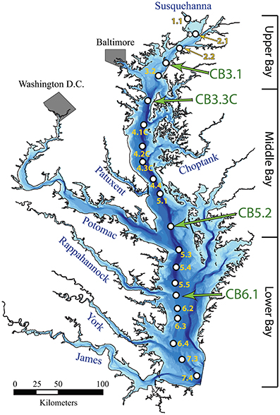
Figure 1. Map of Chesapeake Bay, including key river tributary estuaries and all monitoring stations where data were utilized (note “CB” omitted from station code), including the four stations highlighted in this analysis (CB3.1, CB3.3C, CB5.2, CB6.1).

Interpolation Scheme for Oxygen

We interpolated spatial distributions of dissolved O₂ to a 2-D length-depth grid along the main deep channel using ordinary kriging (Murphy et al., 2010, 2011). The statistical package R with the geoR package (Ribeiro and Diggle, 2001) was used for all interpolations. The resulting 2D distributions were assumed to be constant laterally at a given depth and organized to correspond to tabulated cross-sectional volumes (Cronin and Pritchard, 1975). Interpolated concentration data were multiplied by the cross-sectional volumes to compute “hypoxic volumes” for all available profile sets in the years 1985–2015 by summing the volume of all cells with an O₂ concentration <62.5 μM and <6.25 μM. The threshold values of 62.5 μM (2 mg/L; hypoxic) and 6.25 μM (operationally defined as anoxic) were used to because they have been routinely used in prior research and are thus comparable to past studies, represent a range of values that relevant for a large number (but not all) marine organisms (e.g., Vaquer-Sunyer and Duarte, 2008), and are associated with alterations to biogeochemical processes (Sampou and Kemp, 1994; Testa and Kemp, 2012).

Phenological Metrics of O₂ Depletion

The days of the year where bottom water O₂ concentrations first fall below and rise above the 62.5 μM threshold provide a straightforward index of the amount of time hypoxic conditions persist in a given year. These dates were calculated by (1) averaging bottom-water O₂ concentrations for each sampling date at a single station, (2) interpolating fortnightly and monthly data to obtain daily estimates using shape-preserving piecewise cubic interpolations (i.e., the interpolation is monotonic when data are monotonic and no artificial maxima or minima are generated), and (3) calculating the day when interpolated O₂ concentrations fall below 62.5 μM and then the day they first rise above that value later in summer. Hypoxia onset and breakup dates were calculated for each station in each year from 1985 to 2014.

Generalized Additive Model (GAM) Analyses

GAMs were used to model chlorophyll-a and dissolved inorganic nitrogen at individual stations over time with non-linear smooth functions (Wood, 2006) that allow for changes over time and seasonal cycles to be examined with a statistical approach. In addition, a key component of this GAM implementation is the inclusion of salinity as an explanatory variable to account for the water quality response to short-term freshwater flow events and large-scale inter-annual flow variations (Beck and Murphy, 2017). Extended wet and dry periods in the watershed tend to have a noticeable impact on water quality in Chesapeake Bay, and can make it difficult to discern whether long-term patterns are due to long-term forces, such as management practices being implemented in the watershed, or due to shorter-scale changes of river flow. Including salinity as an explanatory variable and then “adjusting” for it helps remove the variability due solely to freshwater input variations.

Chlorophyll-a and salinity concentrations collected at a single location on the same day were vertically interpolated and averaged to generate a water column mean for each location and day. For dissolved inorganic nitrogen, ammonium (hereafter NH₄+) and nitrate+nitrite (hereafter ${\text{NO}}_{23}^{-}$) were analyzed, as these nitrogen species are the dominant dissolved forms associated with riverine inputs and nutrient recycling in the mainstem of the Bay. Additionally, since our focus is on long-term change, we chose to concentrate our analysis on bottom water concentrations of NH₄+ and ${\text{NO}}_{23}^{-}$ as they are less directly connected with synoptic weather and climate variability. The R package ‘mgcv’ (https://cran.r-project.org/web/packages/mgcv/index.html) was used to fit the following GAM structure separately to the vertically averaged chlorophyll-a, bottom NH₄+ and bottom ${\text{NO}}_{23}^{-}$ data:

$\begin{array}{l}{\text{y}}_{\text{t}}~{\text{y}}_{\text{t}-1}+\text{s}(\text{dyea}{\text{r}}_{\text{t}})+\text{s}(\text{d}\text{o}{\text{y}}_{\text{t}})+\text{s}(\text{s}\text{a}{\text{l}}_{\text{t}})+\text{t}\text{i}(\text{d}\text{o}{\text{y}}_{\text{t}},\text{d}\text{y}\text{e}\text{a}{\text{r}}_{\text{t}})\\ +\text{ti}(\text{do}{\text{y}}_{\text{t}},\text{s}\text{a}{\text{l}}_{\text{t}})+\text{t}\text{i}(\text{s}\text{a}{\text{l}}_{\text{t}},\text{d}\text{y}\text{e}\text{a}{\text{r}}_{\text{t}})+\text{t}\text{i}(\text{d}\text{y}\text{e}\text{a}{\text{r}}_{\text{t}},\text{d}\text{o}{\text{y}}_{\text{t}},\text{s}\text{a}{\text{l}}_{\text{t}})\end{array}$

where y_t represents chlorophyll-a, NH₄+ or ${\text{NO}}_{23}^{-}$ at time t, y_t−1 represents the same parameter at the preceding time step and was included to account for residual autocorrelation, dyear_t is date the sample was collected in a decimal format, doy_t is day of year, sal_t is either the vertical or bottom seasonally-adjusted salinity at the same location, s() indicates a smooth spline function, and ti() indicates a tensor product interaction of two or three spline functions. Thin plate regression splines were used for all variables except a cyclic cubic spline was fit for doy. A cyclic cubic spline allows for predictions to match going from one year to the next, ensuring a smooth seasonal cycle. Otherwise thin plate regression splines were used because of their ability to automatically balance fit and smoothness (Wood, 2006). Tensor products between spline functions allow for an interaction between two variables—allowing, for example, the seasonal cycle to change over time. This model structure was designed to capture the key features in these data sets: long term change (dyear), seasonal cycle (doy), changing seasonal cycles (doy,dyear), a relationship with river flow/salinity (sal), and the ability for the salinity relationship to change over time and season (all ti terms with sal in them). This GAM structure builds from a similar approach in Harding et al. (2015a), who only modeled annual data and hence did not need the seasonal terms, and from Beck and Murphy (2017) who included all of the same parameters, but used a different tensor product construction that does not explicitly show the results from each component separately. GAM results were evaluated in multiple ways. First, any smooth with a p-value greater than 0.1 was dropped from the model to simplify model results as much as possible. Second, the residuals from each model were evaluated graphically to ensure model assumptions of normality, heterogeneity, and independence were met (Wood, 2006). In addition, part of the model fitting involved finding an appropriate data transformation to ensure the normality assumption was met. The Box Cox method (Box and Cox, 1964) was used which allows for either a log-transformation, or additional power transformations if different levels of skewness in the data call for it (see Supplemental Materials). The salinity-adjustment was achieved by running the fitted GAM in prediction mode with an average seasonal cycle for salinity repeated every year for the sal variable. The resulting predictions show estimates of what the parameter of interest would have looked like on certain days of the year throughout the record (April 1 and September 1) if salinity (and hence river flow) had maintained an average seasonal cycle.

Phenological Metrics

To explore the phenology of both nutrient cycling and chlorophyll-a concentrations to understand observed trends in the aforementioned O₂ depletion metrics, several common metrics for characterizing phenology were explored for each year, including: (1) day of maximum concentration, (2) day of minimum concentration, (3) number of days above a known concentration of nutrients associated with water quality impairment (e.g., >0.7 μM N), and (4) day when half the annual integrated concentration was observed during that year. The latter metric proved the most robust measure of timing since it was less susceptible to individual measurements that could determine timing for an entire year.

We created time series of chlorophyll-a, ${\text{NH}}_4^{+}$ and ${\text{NO}}_{23}^{-}$ for those stations and years with at least 10 measurements in a year. Then, we integrated each annual concentration time series over time and determined the day at which half the area under the curve was reached. We used the non-parametric Theil-Sen slope to characterize monotonic trends. The Theil-Sen estimator calculates the median value for all pairwise comparisons between adjacent years and is therefore, relatively robust to outliers (Benson et al., 2012; Dennison et al., 2014). The non-parametric Mann-Kendall trend test was applied to all time series to determine whether trends were significant. All analyses were performed using Matlab R2017a.

Nutrient and Freshwater Input

We analyzed USGS-generated loading estimates for freshwater and nutrients (specifically ${\text{NO}}_{23}^{-}$) based upon fall-line monitoring stations in the Susquehanna and Potomac Rivers (https://cbrim.er.usgs.gov/). To obtain daily concentration and load estimates from nutrient samples taken periodically each month, an approach called Weighted Regressions on Time, Discharge, and Season (WRTDS) was used to estimate nutrient loads (Hirsch et al., 2010; Zhang et al., 2015).

Results

We found regional, season-specific patterns of change in chlorophyll-a, dissolved oxygen, and nutrient concentrations in Chesapeake Bay over the past three decades, consistent with changes in nutrient inputs and physical conditions such as water temperature and stratification. Below we highlight these changes.

Dissolved Oxygen

Mean seasonal cycles of hypoxic and anoxic volume in Chesapeake Bay shifted over the 1985–2015 period, with higher-than-average early summer (May–June) volumes, but lower-than-average late summer (July–September) volumes in the latter half of the time series (2000–2015) relative to the initial period (1985–1999; Figure 2). Hypoxic and anoxic volumes are significantly correlated with January to April Susquehanna+Potomac River flow during all periods (Figure 2). While the timing of hypoxia onset did not change significantly over the 1985-2014 period, the day of hypoxia breakup did become significantly earlier at lower Bay stations CB5.2 and CB6.1 over the 1985–2014 period (Figure 3). At these two stations, the hypoxia breakup day was ~25 days earlier by 2014 than it was at the beginning of the time series. These timing patterns coincide with recent increases in oxygen concentrations in bottom waters for the months of August and September at the majority of stations in the hypoxic region and seaward (data not shown).

FIGURE 2

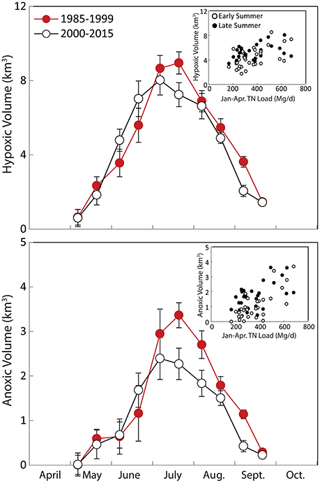
Figure 2. Seasonal cycle of hypoxic and anoxic volumes in Chesapeake Bay, with data divided over the 1985–1999 period (red circles) and 2000–2015 period (green circles). Error bars are standard deviations of the long-term means. Inset is relationship between early summer (May to first half of July) and late summer (late July to September) volumes and January to April Susquehanna plus Potomac Total Nitrogen (TN) loads. Regression statistics for load-hypoxia relationships in inset figures include; early summer hypoxia (adj r² = 0.32, p < 0.001), late summer hypoxia (adj r² = 0.17, p = 0.011), early summer anoxia (adj r² = 0.53, p < 0.001), and late summer anoxia (adj r² = 0.29, p < 0.001).

FIGURE 3

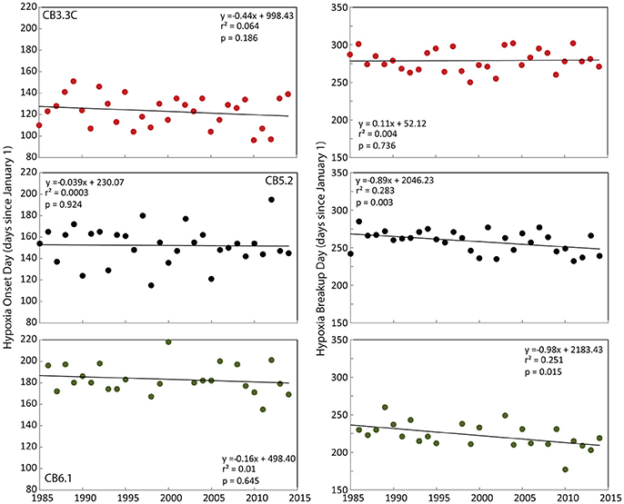
Figure 3. Day of spring hypoxia onset (left panels) and summer/fall hypoxia breakup (right panels) at three stations along the north-south axis of Chesapeake Bay.

Chlorophyll-A

We found long-term trends and altered seasonal cycles of vertically-averaged chlorophyll-a that were quite different between landward (upper Bay) to seaward (lower Bay) stations (Figure 4). During winter-spring, both observations and fitted GAMs from 1985-2016 (Figures 4a,d,g,j) showed a long-term increase in upper bay chlorophyll-a (CB3.1 and CB3.3C) and a fairly constant long-term decline in the mid- and lower-bay (CB5.2 and CB6.1). There also appeared to be a long-term decrease in variability of chlorophyll-a observed at CB5.2 and CB6.1 (Figures 4g,j) with smaller maxima in the most recent two decades (e.g., Figure 4j). It is possible that bloom periods could have been missed in recent years given the 2–4 week sampling frequency of the monitoring program, as modest blooms did occur in a few recent periods (see Supplementary Material). The green and orange lines represent salinity-adjusted estimates of the long-term pattern in April and October, respectively from the GAMs. This approach removes some of the interannual variability that masks phenological change, and the results for the upper bay show an increase in spring concentrations (green lines) and decrease in fall concentrations (oranges lines, Figures 4a,d). In the lower bay, a decrease in spring concentrations is evident, while fall may be slightly increasing (Figures 4g,j). GAM fit statistics (Table 1 and Supplemental Materials) show that the temporal and salinity terms are highly explanatory with low p-values. The R² values show that not all of the variation of the data is explained by these models, but this is expected because our purpose was to identify long-term patterns and general relationships with salinity. A more comprehensive model including some of the many factors that can influence chlorophyll-a concentrations, including climate, nutrients, and mixing, would explain more of the variability. We also analyzed these data with two other techniques to further confirm these findings. For example, separating the time series for each station in half and looking at the mean seasonal cycle from 1985 to 1999 (blue lines in Figures 4b,e,h,k) and 2000–2015 (red lines) shows at upper Bay stations CB3.1 and CB3.3C, the observed long-term increase is due to a large increase in the peak winter-spring concentrations. In contrast, the peak spring concentrations have shifted earlier and are lower in recent years at CB5.2, while at CB6.1, the cycle flattened over time with a noticeably lower spring peak. Finally, at the two upper bay stations, the day of the year when half of the annually integrated chlorophyll-a was observed has moved significantly earlier in the year, as quantified by Thiel-Sen slopes of the time series (Figures 4c,f). The opposite pattern was true in the lower Bay stations, but these changes were not significant.

FIGURE 4

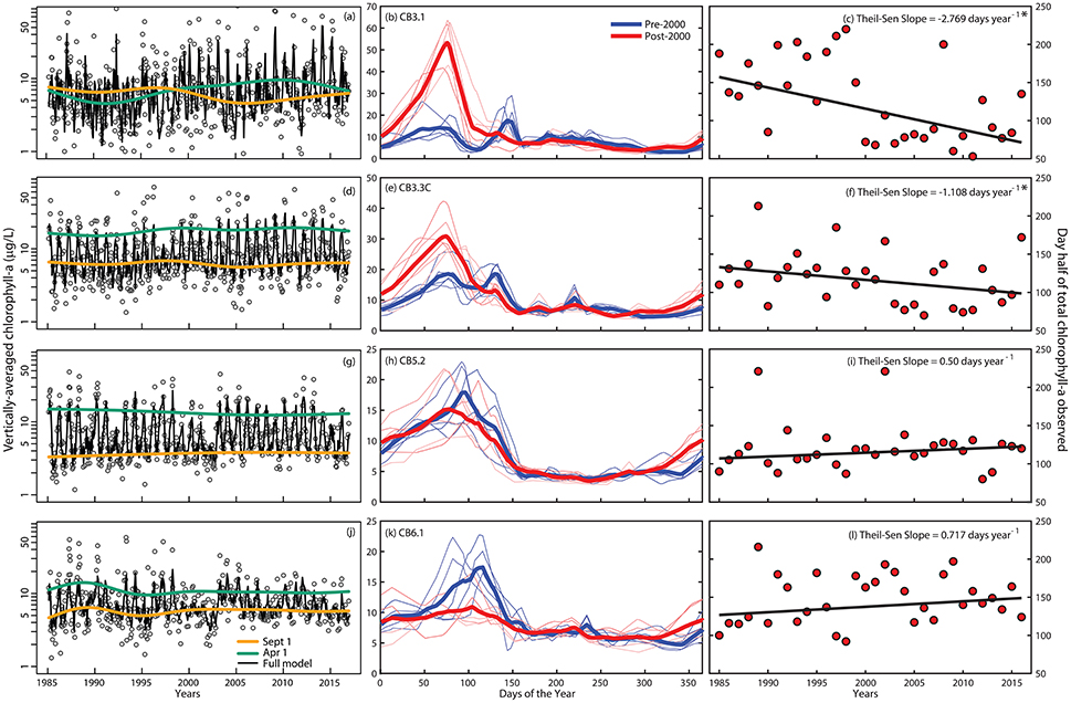
Figure 4. (a,d,g,j) Inter-annual time-series of vertically-averaged water column chlorophyll-a concentrations (natural log scale) with salinity-adjusted smooths for April 1 (green), September 1 (orange), and the full GAM (black lines) at four stations along the salinity gradient in Chesapeake Bay (upper, middle, and lower Bay). (b,e,h,k) Seasonal cycle of vertically-averaged water column chlorophyll-a concentrations with data grouped over 1985–1999 period (light blue lines are means over three sequential groups of years (e.g., 1985–1987, 1988–1990, etc.) and the blue line is the overall mean) and the 2000–2015 period (light red lines are means over three sequential years and the red line is the overall mean). (c,f,i,l) Inter-annual variation and trend in the day of the year when half the vertically-averaged water column chlorophyll-a was observed at each station. Thiel-Sen slopes (e.g., change in concentration per year) are included at the top right, where an * indicates significance (p < 0.05).

TABLE 1

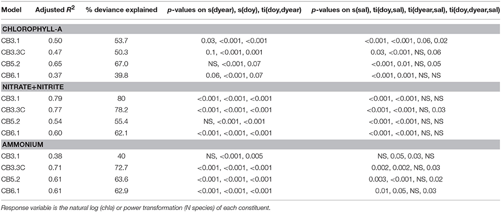
Table 1. Statistics for the GAMs for each parameter and station.

Dissolved Inorganic Nitrogen

We provide the same illustration and analysis of the bottom water ${\text{NH}}_4^{+}$ and ${\text{NO}}_{23}^{-}$ concentrations to illustrate long term patterns and alterations of the seasonal cycle (Figures 5, 6). For ${\text{NH}}_4^{+}$, the day of year when half of the annually integrated ${\text{NH}}_4^{+}$ accumulated has been consistently decreasing from 1985 to 2015 at upper, middle, and lower Bay stations (Figures 5c,f,i,l). The slope of this decrease ranged from −0.82 (CB3.3C) to −1.11 (CB5.2) days per year. The result is that the peak in ${\text{NH}}_4^{+}$ has shifted approximately 1 day per year in the mainstem Chesapeake over the last 30 years. The alteration to the seasonal cycles that cause this shift differs by Bay region. In the upper Bay, this shift in the climatology of bottom water ${\text{NH}}_4^{+}$ appeared to be the result of increasing concentrations in late spring and early summer (Figure 5b), while for the middle and lower Bay, the seasonal shift was realized as a reduction of ${\text{NH}}_4^{+}$ in the late summer-early fall (Figures 5e,h,k). The GAMs (Table 1 and Supplemental Materials) reinforce these findings, as the September salinity-adjusted GAM results (orange lines, Figures 5a,d,g,j) indicate long-term declines, which coincide with the earlier break up in bottom water hypoxia (Figure 3).

FIGURE 5

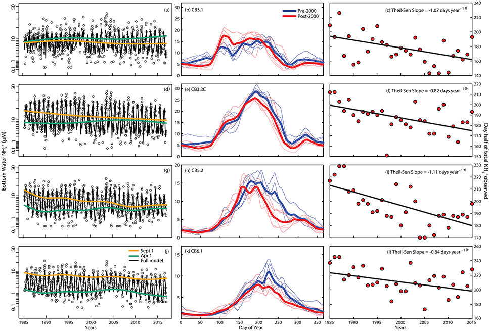
Figure 5. (a,d,g,j) Inter-annual time-series of bottom-water ammonium (${\text{NH}}_4^{+}$) concentrations (transformed scale) with salinity-adjusted smooths for April 1 (green) and September 1 (orange), and the full GAM (black line) at four stations along the salinity gradient in Chesapeake Bay. (b,e,h,k) Seasonal cycle of bottom-water ammonium concentrations with data grouped over 1985–1999 period (light blue lines are means over three sequential groups of years (e.g., 1985–1987, 1988–1990, etc.) and the blue line is the overall mean) and the 2000–2015 period (light red lines are means over three sequential groups of years and the red line is the overall mean). (c,f,i,l) Inter-annual variation and trend in the day of the year when half the bottom-water ammonium was observed at each station. Thiel-Sen slopes (e.g., change in concentration per year) are included at the top right, where an * indicates significance (p < 0.05).

FIGURE 6

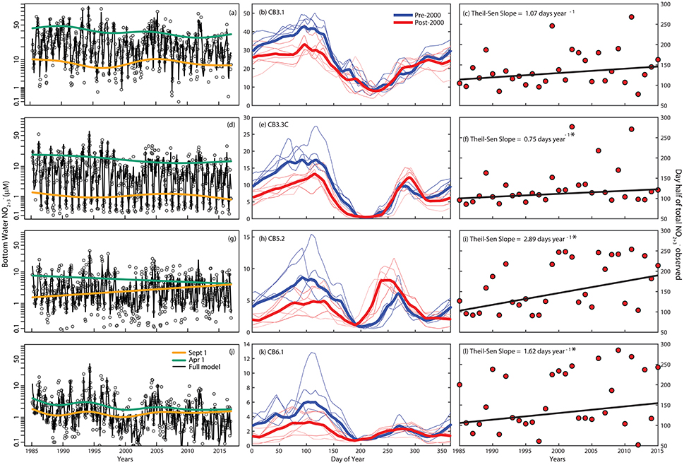
Figure 6. (a,d,g,j) Inter-annual time-series of bottom-water nitrate + nitrite (${\text{NO}}_{23}^{-}$) concentrations (transformed scale) with salinity-adjusted smooths for April 1 (green), September 1 (orange), and the full GAM (black line) at four stations along the salinity gradient in Chesapeake Bay. (b,e,h,k) Seasonal cycle of bottom-water nitrate + nitrite concentrations with data grouped over 1985–1999 period (light blue lines are means over three sequential groups of years (e.g., 1985–1987, 1988–1990, etc.) and the blue line is the overall mean) and the 2000–2015 period (light red lines are means over three sequential groups of years and the red line is the overall mean). (c,f,i,l) Inter-annual variation and trend in the day of the year when half the bottom-water nitrate + nitrite was observed at each station. Thiel-Sen slopes (e.g., change in concentration per year) are included at the top right, where an * indicates significance (p < 0.05).

Long-term changes in the seasonal patterns of bottom-water ${\text{NO}}_{23}^{-}$ also show distinct patterns over multiple regions of Chesapeake Bay. Trends in the day of year when half of the annually integrated ${\text{NO}}_{23}^{-}$ has been observed are largely the inverse of trends in ${\text{NH}}_4^{+}$, where these dates occurred consistently later in the annual cycle (Figures 6c,f,i,l). The trends indicate that the peak in ${\text{NO}}_{23}^{-}$ is getting later in the year at all stations except CB3.1, including the majority of the mid-and lower Bay stations (Figures 6b,e,h,k; Supplemental Materials). The change in ${\text{NO}}_{23}^{-}$ timing was consistently associated with a decline in winter-spring ${\text{NO}}_{23}^{-}$ concentrations (which also occurred in surface waters; data not shown), which occurred at all stations (Figures 6b,e,h,k). The magnitude of the decline between the two time periods (1985–1999 vs. 2000–2015) increased down the mainstem of the Bay: 23% (CB3.1), 33% (CB3.3.C), 43% (CB5.2), and 81% (CB6.1). At two stations in the middle and lower Bay (CB3.3C and CB5.2), the seasonal cycle was further flattened because the late summer-fall ${\text{NO}}_{23}^{-}$ was higher in the most recent two decades (Figures 6e,h), a pattern that was consistent across stations across the mid- and lower-Bay (see Supplemental Materials). Further demonstrating this point, the salinity-adjusted GAM results show a downward trend in the April salinity-adjusted predictions with increasing magnitude from upper to lower Bay (Figures 6a,d,g,i).

Total Nitrogen Loading

We also analyzed long-term changes in nutrient loading that were associated with declines in chlorophyll-a and dissolved nitrogen concentration. Direct inputs of ${\text{NO}}_{23}^{-}$ to the Chesapeake estuary mainstem (where our analysis is focused) are primarily driven by flows from the Susquehanna River. While high interannual variability in river flow tends to dominate variation in ${\text{NO}}_{23}^{-}$ inputs, Susquehanna ${\text{NO}}_3^{-}$ loads have declined recently due to declines in N concentrations in the Susquehanna and other rivers (Zhang et al., 2015). The primary season where loads have declined is the winter-spring, where ${\text{NO}}_3^{-}$ loads were 20–30% lower during February to April in 2000–2015 relative to 1985–1999 (Figure 7). While the September ${\text{NO}}_3^{-}$ loads appear to be higher on average in recent decades, this high September value is primarily driven by an extraordinary high load during the combined effects of Tropical storms Irene and Lee driving historic Susquehanna River flow during September 2011 (Figure 7). A time-series of February to April mean ${\text{NO}}_3^{-}$ load indicates a long-term decline that is not significant (r = 0.27, p = 0.134; top panel of Figure 7), but the ${\text{NO}}_3^{-}$ load generated for a given river flow in 2000–2015 is significantly lower than for 1985–1999 (ANCOVA; F = 10.81, p = 0.0028; Figure 7).

FIGURE 7

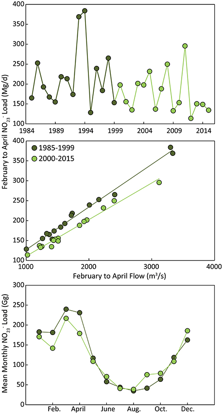
Figure 7. Top: Time-series of mean February to April Susquehanna River nitrate+nitrite loads for the 1985–2015 period. Middle: Relationship between mean February to April river flow and nitrate+nitrite loading with data separated into two subsequent periods. Bottom: Mean seasonal cycle of Susquehanna River nitrate+nitrite loads for two subsequent periods.

Temperature and Stratification

To understand changes in biogeochemical variables in relation to climatically-driven physical changes in the estuary, we analyzed measurements of temperature and salinity to compute temporal changes in both water temperature and the Brunt-Vaisala Frequency (BVF), a measure of the strength of stratification (Figures 7, 8). We illustrate the statistical results (correlation coefficient, p-value) for correlations between year and metrics of temperature and stratification as time-space contour plots (i.e., Hovmöller diagrams) that indicate where significant long-term change occurred over space and season (Figures 7, 8). For temperature, we examined the trend in the monthly deviation from the long-term mean surface temperature, which indicated that significant long-term increases in temperature primarily occurred during April in the upper Bay (CB2.1 to CB3.1) and during June and July throughout the majority of the mainstem Bay (Figure 8). The slopes of these linear regressions indicate increases of 0.025 to 0.05°C per year, or 0.7 to 1.5°C increases over 30 years in regions where increases were significant. For stratification, long-term changes in maximum BVF were absent for the majority of months and regions in the Bay. The only significant increases occurred during March in the upper and lower Bay and during June in a limited region of the upper Bay (Figure 9). Summer and fall BVF did not change over the 1985–2015 period, and there was no change in the depth of maximum BVF at any station during any particular season.

FIGURE 8

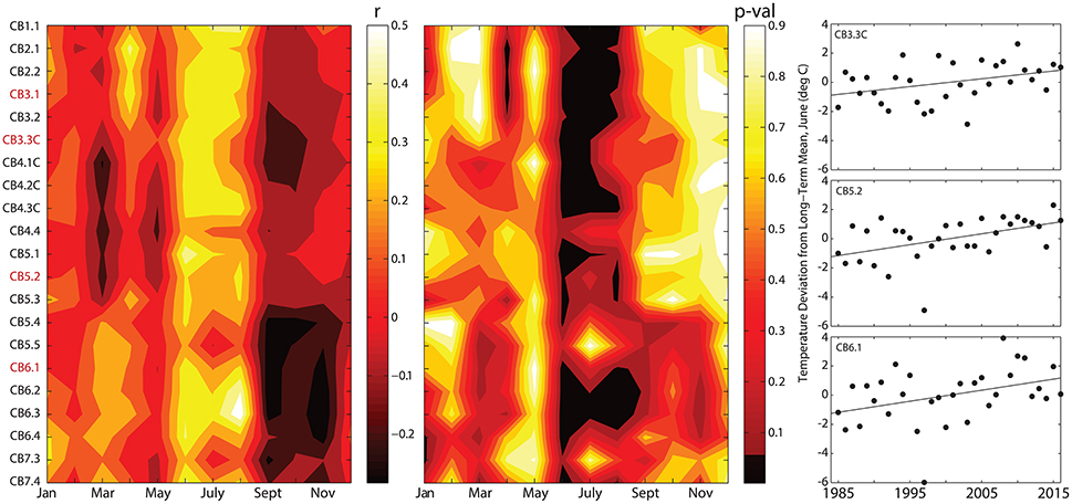
Figure 8. Time-space contour plots (i.e., Hovmöller diagrams) showing r values (Left) and p-values (Middle) for correlations between year and monthly deviations from long-term monthly averages for surface water temperature at all mainstem Bay sampling stations spanning the north-south axis of the Bay (CB1.1 = northern extent, CB7.4 = southern extent; see Figure 1). The plots indicate which regions and months include significant long-term changes. The time series in the far right panel show deviation from long-term monthly means for the month of June at three stations. For p-values, black indicates stations and months with significant increases (p < 0.05). Stations in red are those highlighted in Figures 3–6.

FIGURE 9

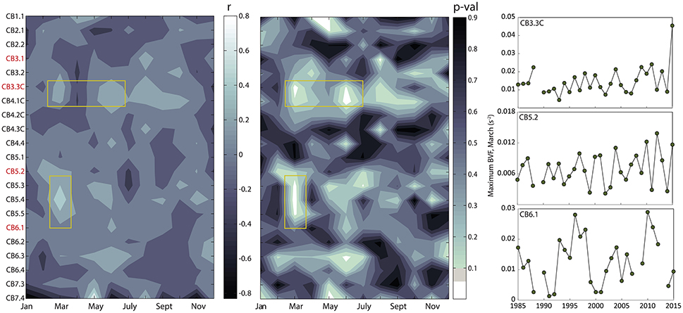
Figure 9. Time-space contour plots (i.e., Hovmöller diagrams) showing r values (Left) and p-values (Middle) for correlations between year and the monthly maximum Brunt-Vaisala Frequency (BVF), a measure of the strength of stratification, at all mainstem Bay sampling stations spanning the north-south axis of the Bay (CB1.1 = northern extent, CB7.4 = southern extent; see Figure 1). The plots indicate which regions and months include significant long-term changes. The time series in the far right panel shows BVF for the month of March at three middle and lower Bay stations. For p-values, white indicates stations and months with significant increases (p < 0.05). Stations in red are those highlighted in Figures 3–6.

Discussion

Our analysis highlights season-specific, long-term changes in the concentrations of chlorophyll-a, O₂, and dissolved inorganic nitrogen along the north-south axis of Chesapeake Bay. We illustrate these long-term changes as alterations to the seasonal cycles of these variables that have occurred relatively gradually over the past 30 years, suggesting a change in estuarine phenology. The concepts of phenology apply to the myriad recurring seasonal phenomena in Chesapeake Bay and other estuaries and coastal waters, such as the timing of the spring bloom, development of seasonal hypoxia, and the annual availability and cycling of key nutrients. Clear linkages in the production and consumption of these variables underscore their coupled changes in response to nutrient load reductions, temperature increases, and oxygen depletion.

The most integrative alteration of a seasonal cycle we examined included a shift toward larger hypoxic volumes in spring-early summer and smaller volumes during late summer-fall over the past 30 years (Murphy et al., 2011; Zhou et al., 2014; Testa et al., 2017). This springward shift in the maximum hypoxic volume did not correspond to significantly earlier hypoxia onset in the upper Bay (Figure 3), which has been shown to be strongly related to winter spring freshwater inputs and local bottom-water chlorophyll-a (Testa and Kemp, 2014). The earlier seasonal shift did, however, correspond to an earlier breakup of hypoxia at the end of the warm season (Figure 3) and elevated bottom-water oxygen concentrations in August and September, including lower anoxic volumes in the late summer (Testa et al., 2017). Various metrics of re-oxygenation in the late summer reveal that the most prominent increases in oxygen availability have occurred in seaward Bay waters south of the Potomac River. Due to the bathymetry of Chesapeake Bay, periods of high nutrient loading tend to result in a seaward expansion in hypoxic volume as opposed to uniform increase in hypoxic volume in all directions (Murphy et al., 2011; Testa et al., 2014). Thus, we expect this region to be an early indicator of recovery from eutrophication. Reoxygenation of lower Bay waters also feeds back to support more up-Bay advective input of O₂ associated with gravitational circulation, leading to more oxygenation in landward regions (Testa et al., in press). Thus, if oxygen concentrations increase in lower Bay waters, the reoxygenation signal can be transmitted to other regions of the estuary.

Considering first the oxygen dynamics during the latter half of the summer, conceptual models of eutrophication suggest that nutrient inputs fuel increases in phytoplankton growth and biomass that ultimately sustain respiratory processes that consume O₂ (e.g., Kemp et al., 2005). Consequently, we would expect that reductions in nutrient input should lead to lower rates of oxygen consumption and less hypoxia, given similar physical conditions. The reduction in late summer hypoxia and anoxia corresponds to declines in nitrogen loading from the majority of the Chesapeake watershed (Zhang et al., 2015). This includes reductions in ${\text{NO}}_{23}^{-}$ loads from the Susquehanna River, which is the largest source of nutrients to the estuary during February-April (Figure 7). While these load reductions are modest, water-column concentrations of total nitrogen (Lefcheck et al., 2018) and winter-spring ${\text{NO}}_{23}^{-}$ (Figure 6) have declined significantly over the past 30 years in the majority of the Chesapeake Bay main stem. Clearly the availability of nitrogen has declined during the winter-spring period when high phytoplankton net metabolism and biomass accumulation in Chesapeake Bay typically occur (Smith and Kemp, 1995; Harding and Perry, 1997).

Although the decline in late-summer hypoxia and anoxia has been hypothesized to be linked to reduced winter-spring nutrient inputs and, presumably, reduced phytoplankton biomass (Murphy et al., 2011), the linkages between these processes has yet to be established in space and time. At several stations in the Bay south of the Potomac River, March-May water-column chlorophyll-a concentrations have declined over time, and higher values in excess of 10 μg/L were rare in the most recent decade (Figure 4). This reduction in chlorophyll-a under reduced nitrogen availability is consistent with bioassays that suggest nitrogen limitation in seaward Chesapeake Bay waters during this period (Fisher et al., 1999). Although not a focus of this study, phosphorus has also declined over this timeframe in some tidal waters (Lefcheck et al., 2018) and has also been shown to be limiting in bioassays as well (Fisher et al., 1999). If we extrapolate chlorophyll-a concentrations from the stations to regional values with surface areas and volumes for Chesapeake Bay (Cronin and Pritchard, 1975), the upper Bay would have contributed ~3–10% of baywide chlorophyll-a before 1999, but in the most recent 15 years the upper Bay contribution increased to ~15–20% (and the lower Bay declined from ~50 to ~30%). Consequently, we would expect that less organic matter was available in the lower Bay to maintain respiration later into summer, allowing oxygen concentrations to increase in this region and during this time. Given that late-summer ${\text{NH}}_4^{+}$ concentrations have declined substantially throughout the mid and lower Bay over the past-30 years (Figure 5), it appears that some combination of enhanced retention and recycling in the upper Bay (Figure 5b), enhanced early summer recycling (accelerated by higher temperature), and reduced organic material to support recycling (as assumed given reduced April-May chlorophyll-a; Figure 4k) contributed to the ${\text{NH}}_4^{+}$ decline.

Another factor involved in the long-term reduction in bottom-water ${\text{NH}}_4^{+}$ could be elevated nitrification in response to reoxygenation (Testa et al., in press). Increases in the concentration of ${\text{NO}}_{23}^{-}$ (which includes nitrite, ${\text{NO}}_2^{-}$) during late-summer in the bottom-layer of portions of the middle and lower Bay (Figure 6, Supplementary Material) occurred despite long-term reductions in total nitrogen inputs (Figures 6, 7). Past studies have measured high rates of nitrification and ${\text{NO}}_2^{-}$ accumulation in the late summer and early fall during fall turnover, a period when high ${\text{NH}}_4^{+}$ water is oxygenated via vertical mixing, thus stimulating nitrification (McCarthy et al., 1984; Horrigan et al., 1990). Given the long-term increase in oxygen concentrations observed in the bottom-waters of the seaward regions of the Bay, we expect elevated nitrification rates would explain a portion of the ${\text{NH}}_4^{+}$ decline and the increase in ${\text{NO}}_{23}^{-}$. Recent studies have shown that such a pathway is sufficiently large to link the opposing temporal trends of ${\text{NH}}_4^{+}$ and ${\text{NO}}_{23}^{-}$ (Testa et al., in press), underscoring the fact that bioavailable nitrogen in Chesapeake Bay changes seasonally (${\text{NO}}_{23}^{-}$ in spring and fall, ${\text{NH}}_4^{+}$ in summer) and that changes in oxygen availability feedback to alter the seasonal cycle of nitrogen speciation, where nitrogen load reductions have directly led to lower winter-spring ${\text{NO}}_{23}^{-}$, but indirectly led to increased late summer/fall ${\text{NO}}_{23}^{-}$ (associated with reoxygenation).

As for the observed increase in hypoxic volume during early summer (Figure 2), we considered both climatic and biological factors. Elevated summer temperatures are expected to alter patterns of hypoxia, and consequently, the availability of ${\text{NH}}_4^{+}$ in Chesapeake Bay (Najjar et al., 2010; Testa and Kemp, 2012). We documented clear increases in summer temperatures throughout Chesapeake Bay waters, which are consistent with recent analyses in Chesapeake Bay (Kaushal et al., 2010; Ding and Elmore, 2015), the northern Gulf of Mexico, and Narragansett Bay (Nixon et al., 2004; Turner et al., 2017). While most prior discussions have emphasized the impact of elevated temperature on respiration rates and solubility to conclude that future warming should increase hypoxia (Najjar et al., 2010; Altieri and Gedan, 2015), the impact of warming is likely more nuanced. For example, recent warming (Figure 8) could be expected to increase the rate of respiration of organic matter by 15–20% at a 2°C increase (using organic matter oxidation formulations as in Testa et al., 2014), thereby recycling nitrogen from organic matter (as ${\text{NH}}_4^{+}$) earlier in the summer. Previous studies have revealed that mid-Chesapeake Bay sediments have historically been starved of labile organic material (i.e., by measuring reduced sediment-water ${\text{NH}}_4^{+}$ fluxes) by late-summer (Boynton and Kemp, 2008; Brady et al., 2013). Thus, if respiration rates increase due to temperature, we expect that organic matter generated during spring would be exhausted even earlier in the summer. Therefore, more oxygen would be consumed earlier in the year (and less later in the year). In fact, our observations of a seasonal shift toward earlier maximum hypoxic volumes and earlier exhaustion of ${\text{NH}}_4^{+}$ pools are consistent with temperature-induced increases in the rate of organic matter degradation in early summer.

In contrast to the seaward regions of the estuary, the more landward, low salinity regions (upper Bay) were characterized by elevated chlorophyll-a and bottom-water ${\text{NH}}_4^{+}$, but no change in timing of hypoxia onset and breakup. Chlorophyll-a increases appear to be focused in the November to March period, where chlorophyll-a has more than doubled (with mean values of 9.3 μg L⁻¹ in 1985–1999 vs. 19.3 μg L⁻¹ in 2000–2016) over time averaged at stations CB3.1 and CB3.3C. Recent analysis of long-term changes in phytoplankton community composition over this same timeframe have suggested that dinoflagellates have become an increasing portion of phytoplankton biomass, whereas previously the composition was dominated by diatoms (Harding et al., 2015b). Winter blooms of dinoflagellates have been documented in the estuarine turbidity maximum region of the main stem Chesapeake Bay, in the vicinity of the CB3.1 (Lee et al., 2012), as well as in multiple tributaries of Chesapeake Bay (Sellner et al., 1991; Millette et al., 2015). Many of these species tend to be mixotrophic, using phagotrophy as an alternative energy acquisition strategy during winter-spring in turbid waters, where low light availability limits photoautotrophy (Millette et al., 2017). The moderate increases in stratification (and presumably lower turbulence) we confirmed during this season in the landward Bay regions would likely favor these small, flagellated organisms (Margalef, 1978; Hinder et al., 2012). While mixotrophic strategies for carbon acquisition would somewhat decouple these communities from external nutrient loads, any nutrient uptake by these organisms, if increasing, would limit the seaward flux of nutrients and increase the effect of watershed nutrient load reductions (Paerl et al., 2004). The increase in upper Bay chlorophyll-a could also be linked to increases in total phosphorus loading from the Susquehanna River (Zhang et al., 2015), because this region of the Bay in winter-spring can be phosphorus limited (Fisher et al., 1999). Regardless of the causes of the increase in chlorophyll-a, the increase is associated with elevated ${\text{NH}}_4^{+}$ accumulation during early summer in upper Bay bottom waters, which represents a distinct springward shift (Figure 5). In addition, the larger hypoxic volumes in the early summer would be expected from the upper bay chlorophyll-a increase, given that the oxygen depletion in the early summer tends to be restricted to more landward Bay waters.

Our analysis included a separation of the concentration time-series into two distinct periods, which represent a relatively even division of the 30 year time-series. Although we emphasize that the concentration changes were generally gradual for most of these variables (Figures 3–6), several important features of external forcing in Chesapeake Bay occurred around the year 2000 that could cause more abrupt changes. First, a prolonged four-year drought lasted from 1999 to 2002, which is associated with persistently low nutrient loading that coincided with key biological changes in the estuary, including an expansion of a large submerged aquatic vegetation (SAV) bed (Gurbisz and Kemp, 2014; Orth et al., 2017), the aforementioned changes in phytoplankton composition, and the increase in upper Bay chlorophyll-a. Increases in the biomass of both SAV and phytoplankton after 2000 would lead to increased retention of dissolved nutrients in the upper Bay, and associated reductions in seaward nutrient transport to support phytoplankton growth in the lower Bay. Secondly, a large reservoir system at the mouth of the Susquehanna River reached a threshold of infill around 2000 that initiated a relatively abrupt and persistent increase in the concentration of fine suspended sediments and associated particulate nutrient loading for a given freshwater input (Cerco and Noel, 2016; Zhang et al., 2016), which could have contributed to increased light attenuation in the upper Bay. While it is possible that reduced light availability contributed to altered carbon to chlorophyll ratios in the phytoplankton that caused elevated chlorophyll-a without associated increases in biomass, chlorophyll-a concentrations in the upper Bay were significantly correlated with water-column particulate nitrogen and phosphorus (PN, PP, respectively) concentrations over the entire data record [r² = 0.91, (PN), r² = 0.38 (PP), p < 0.01], suggesting that this was not the case. Our analysis of stratification did not suggest any clear changes over this timeframe in the lower Bay that would have strongly impacted the reductions we observed in phytoplankton biomass during spring or the increases in oxygen availability observed during late summer. Future investigations using targeted field and modeling analyses will improve our understanding of how seasonal cycles and spatial gradients modulate biogeochemical coupling of key elements in estuarine ecosystems.

Summary

Overall, our findings reveal not only a seasonal shift toward earlier peaks in chlorophyll-a and oxygen depletion, but also a spatial shift toward more phytoplankton biomass in upper Bay regions and less biomass in seaward regions. The north-ward and winter-ward migration of the spring bloom would increase phytoplankton-derived organic matter deposition in the upper Bay at the expense of the lower Bay, which should increase the volume of early season hypoxia but reduce late season volumes and cause an earlier hypoxia breakup. No clear change in physical forcing was evident from our analysis of stratification that could have caused the late summer reoxygenation, and previous model simulations have shown a high dependence of hypoxic volume on early summer water-column respiration. A decreasing trend in winter-spring ${\text{NO}}_{23}^{-}$ (attributable to decreasing nutrient loading the Bay) and late summer ammonium oxidation (attributable to reduced organic material and an earlier break-up of the hypoxic zone) appear to corroborate the dynamics reported for chlorophyll-a and O₂ depletion. These results emphasize that changes to nutrient loading, water temperature, and other external forcing have conspired to drive long-term changes in key seasonal phenomenon like the spring bloom and summer hypoxia, which are linked through coupled carbon, oxygen, and nitrogen cycling. Our ability to detect these changes resulted from the phenology-specific nature of our analysis, which allowed us to clearly observe biogeochemical changes that were realized through altered seasonal cycles. In summary we emphasize the following conclusions and hypotheses. (a) It is useful to examine seasonal changes in biogeochemical variables (altered phenology) as a feature of monitoring and explaining long-term trends. (b) We highlight that changes in the seasonality of hypoxia can be reasonably explained by large seasonal and regional shifts in phytoplankton biomass and physical conditions (e.g., temperature). (c) We also expect future changes in climate and nutrient loading to continue to influence the seasonality of linked biogeochemical cycles in estuarine ecosystems.

Author Contributions

JT: led the writing of the manuscript and helped design the research; JT: contributed several figures to the manuscript and performed many of the analyses; RM: contributed to writing the manuscript, helped design the research, performed GAM analysis, contributed figures; DB: contributed to writing the manuscript, helped design the research, performed time-series analysis, contributed figures; WK: contributed to writing the manuscript and advised in the research design.

Conflict of Interest Statement

The authors declare that the research was conducted in the absence of any commercial or financial relationships that could be construed as a potential conflict of interest.

Acknowledgments

Support from several grants and contracts have made this research possible, including the US National Science Foundation grants (i) DEB1353766 (OPUS; WK), (ii) 11A-1355457 (DB), and (iii) CBET1360415 (WSC; JT, DB, and WK), (iv) US National Oceanic and Atmospheric Administration (NOAA) grant NA15NOS4780184 (JT and WK) and (v) U.S. Environmental Protection Agency grant 07-5-230480 (RM). This is contribution # 5483 from the University of Maryland Center for Environmental Science. Data used in this research were provided by the Chesapeake Bay Program and the Maryland Department of Natural Resources.

Supplementary Material

The Supplementary Material for this article can be found online at: https://www.frontiersin.org/articles/10.3389/fmars.2018.00114/full#supplementary-material

References

Altieri, A. H., and Gedan, K. B. (2015). Climate change and dead zones. Global Change Biol. 21, 1395–1406. doi: 10.1111/gcb.12754

PubMed Abstract | CrossRef Full Text | Google Scholar

Beck, M. W., and Murphy, R. R. (2017). Numerical and qualitative contrasts of two statistical models for water quality change in tidal waters. JAWRA J. Am. Water Res. Assoc. 53, 197–219. doi: 10.1111/1752-1688.12489

CrossRef Full Text | Google Scholar

Benson, B. J., Magnuson, J. J., Jensen, O. P., Card, V. M., Hodgkins, G., Granin, N. G., et al. (2012). Extreme events, trends, and variability in Northern Hemisphere lake-ice phenology. Clim. Change 112, 299–323. doi: 10.1007/s10584-011-0212-8

CrossRef Full Text | Google Scholar

Box, G. E. P., and Cox, D. R. (1964). An analysis of transformations. J. R. Stat. Soc. Ser. B 26, 211–252.

Google Scholar

Boynton, W. R., and Kemp, W. M. (2008). “Estuaries,” in Nitrogen in the Marine Environment, eds D. G. Capone, D. A. Bronk, M. R. Mulholland and E. J. Carpenter (Amsterdam: Elsevier), 809–866.

Brady, D. C., Testa, J. M., Di Toro, D. M., Boynton, W. R., and Kemp, W. M. (2013). Sediment flux modeling: calibration and application for coastal systems. Estuar. Coast. Shelf Sci. 117, 107–124. doi: 10.1016/j.ecss.2012.11.003

CrossRef Full Text | Google Scholar

Cerco, C. F., and Noel, M. R. (2016). Impact of reservoir sediment scour on water quality in a downstream estuary. J. Environ. Qual. 45, 894–905. doi: 10.2134/jeq2014.10.0425

PubMed Abstract | CrossRef Full Text | Google Scholar

Cloern, J. E., Jassby, A. D., Thompson, J. K., and Hieb, K. A. (2007). A cold phase of the east pacific triggers new phytoplankton blooms in San Francisco bay. Proc. Natl. Acad. Sci. U.S.A. 104, 18561–18565. doi: 10.1073/pnas.0706151104

PubMed Abstract | CrossRef Full Text | Google Scholar

Costello, J. H., Sullivan, B. K., and Gifford, D. J. (2006). A physical–biological interaction underlying variable phenological responses to climate change by coastal zooplankton. J. Plank. Res. 28, 1099–1105. doi: 10.1093/plankt/fbl042

CrossRef Full Text | Google Scholar

Cronin, W. B., and Pritchard, D. W. (1975). Additional Statistics on the Dimensions of Chesapeake Bay and its Tributaries: Cross-Section Widths and Segment Volumes per Meter depthRep. Baltimore, MD: Chesapeake Bay Institute, The Johns Hopkins University.

Dennison, P. E., Brewer, S. C., Arnold, J. D., and Moritz, M. A. (2014). Large wildfire trends in the western United States, 1984-2011. Geophys. Res. Lett. 41, 2928–2933. doi: 10.1002/2014GL059576

CrossRef Full Text | Google Scholar

Ding, H., and Elmore, A. J. (2015). Spatio-temporal patterns in water surface temperature from Landsat time series data in the Chesapeake Bay, USA. Remote Sens. Environ. 168, 335–348. doi: 10.1016/j.rse.2015.07.009

CrossRef Full Text | Google Scholar

Fisher, T. R., Gustafson, A. B., Sellner, K., Lacouture, R., Haas, L. W., Karrh, R., et al. (1999). Spatial and temporal variation of resource limitation in Chesapeake Bay. Mar. Biol. 133, 763–778. doi: 10.1007/s002270050518

CrossRef Full Text | Google Scholar

Guinder, V. A., Popovich, C. A., Molinero, J. C., and Perillo, G. M. E. (2010). Long-term changes in phytoplankton phenology and community structure in the Bahía Blanca Estuary, Argentina. Mar. Biol. 157, 2703–2716. doi: 10.1007/s00227-010-1530-5

CrossRef Full Text | Google Scholar

Gurbisz, C., and Kemp, W. M. (2014). Unexpected resurgence of a large submersed plant bed in Chesapeake Bay: analysis of time series data. Limnol. Oceanogr. 59, 482–494. doi: 10.4319/lo.2014.59.2.0482

CrossRef Full Text | Google Scholar

Hagy, J. D., Boynton, W. R., Keefe, C. W., and Wood, K. V. (2004). Hypoxia in Chesapeake Bay, 1950-2001: long-term change in relation to nutrient loading and river flow. Estuaries 27, 634–658. doi: 10.1007/BF02907650

CrossRef Full Text | Google Scholar

Harding, L. W., Adolf, J. E., Mallonee, M. E., Miller, W. D., Gallegos, C. L., Paerl, H. W., et al. (2015b). Climate effects on phytoplankton floral composition in Chesapeake Bay. Estuar. Coast. Shelf Sci. 162, 53–68. doi: 10.1016/j.ecss.2014.12.030

CrossRef Full Text | Google Scholar

Harding, L. W., Gallegos, C. L., Perry, E. S., Miller, W. D., Adolf, J. E., Paerl, H. W., et al. (2015a). Long-term trends of nutrients and phytoplankton in Chesapeake Bay, Estuar. Coas. 39, 664–681. doi: 10.1007/s12237-015-0023-7

CrossRef Full Text | Google Scholar

Harding, L. W., and Perry, E. (1997). Long-term increase of phytoplankton biomass in Chesapeake Bay, 1950-1994. Mar. Ecol. Prog. Ser. 157, 39–52. doi: 10.3354/meps157039

CrossRef Full Text | Google Scholar

Hinder, S. L., Hays, G. C., Edwards, M. E., Roberts, E. C., Walne, A. W., and Gravenor, M. B. (2012). Changes in marine dinoflagellate and diatom abundance under climate change. Nat. Clim. Change 2, 271–275. doi: 10.1038/nclimate1388

CrossRef Full Text | Google Scholar

Hirsch, R. M., Moyer, D. L., and Archfield, S. A. (2010). Weighted regressions on time, discharge, and season (WRTDS), with an application to Chesapeake Bay river inputs. J. Am. Water Res. Assoc. 46, 857–880. doi: 10.1111/j.1752-1688.2010.00482.x

PubMed Abstract | CrossRef Full Text | Google Scholar

Horrigan, S. G., Montoya, J. P., Nevins, J. L., McCarthy, J. J., Ducklow, H., Malone, T., et al. (1990). Nitrogenous nutrient transformations in the spring and fall in the Chesapeake Bay. Estuar. Coast. Shelf Sci. 30, 369–391. doi: 10.1016/0272-7714(90)90004-B

CrossRef Full Text | Google Scholar

Jahan, R., and Choi, J. K. (2014). Climate regime shift and phytoplankton phenology in a macrotidal estuary: long-term surveys in Gyeonggi Bay, Korea. Estuar. Coasts 37, 1169–1187. doi: 10.1007/s12237-013-9760-7

CrossRef Full Text | Google Scholar

Jeong, S.-J. C., Ho, H. H., Gim, J., and Brown, M. E. (2011). Phenology shifts at start vs. end of growing season in temperate vegetation over the Northern Hemisphere for the period 1982–2008. Global Change Biol. 17, 2385–2399. doi: 10.1111/j.1365-2486.2011.02397.x

CrossRef Full Text | Google Scholar

Johnson, Z., Bennett, M., Linker, L., Julius, S., Najjar, R., Mitchell, M., et al. (2016). The Development of Climate Projections for Use in Chesapeake Bay Program AssessmentsRep (Edgewater, MD: STAC, Chesapeake Bay Program), 52.

Kaushal, S. S., Likens, G. E., Jaworski, N. A., Pace, M. L., Sides, A. M., Wingate, R. L., et al. (2010). Rising stream and river temperatures in the United States. Front. Ecol. Environ. 8, 461–466. doi: 10.1890/090037

CrossRef Full Text | Google Scholar

Kemp, W. M., Boynton, W. R., Adolf, J. E., Boesch, D. F., Boicourt, W. C., Brush, G., et al. (2005). Eutrophication of Chesapeake Bay: historical trends and ecological interactions, Mar. Ecol. Prog. Ser. 303, 1–29. doi: 10.3354/meps303001

CrossRef Full Text | Google Scholar

Lee, D. Y., Keller, D., Crump, B. C., and Hood, R. R. (2012). Community metabolism and energy transfer in the Chesapeake Bay estuarine turbidity maximum. Mar. Ecol. Prog. Ser. 449, 65–82. doi: 10.3354/meps09543

CrossRef Full Text | Google Scholar

Lefcheck, J. S., Orth, R. J., Dennison, W. C., Wilcox, D. J., Murphy, R. R., Keisman, J., et al. (2018). Long-term nutrient reductions lead to the unprecedented recovery of a temperate coastal region. Proc. Natl. Acad. Sci. U.S.A. doi: 10.1073/pnas.1715798115. [Epub ahead of print].

PubMed Abstract | CrossRef Full Text | Google Scholar

Li, M. Y., Lee, J., Testa, J. M., Li, Y., Ni, W., Toro, D. M. D., et al. (2016). What drives interannual variability of estuarine hypoxia: climate forcing versus nutrient loading?. Geophys. Res. Lett. 43, 2127–2134. doi: 10.1002/2015GL067334

CrossRef Full Text | Google Scholar

Li, M., and Zhong, L. (2009). Flood-ebb and spring-neap variations of mixing, stratification and circulation in Chesapeake Bay. Cont. Shelf Res. 29, 4–14. doi: 10.1016/j.csr.2007.06.012

CrossRef Full Text | Google Scholar

Li, Y., Li, M., and Kemp, W. M. (2015). A budget analysis of bottom-water dissolved oxygen in Chesapeake Bay. Estuar. Coasts 38, 2132–2148. doi: 10.1007/s12237-12014-19928-12239

CrossRef Full Text | Google Scholar

Margalef, R. (1978). Life-forms of phytoplankton as survival alternatives in an unstable environment. Oceanol. Acta 1, 493–509.

Google Scholar

McCarthy, J. J., Kaplan, W., and Nevins, J. L. (1984). Chesapeake Bay nutrient and plankton dynamics. 2. sources and sinks of nitrite. Limnol. Oceanogr. 29, 84–98. doi: 10.4319/lo.1984.29.1.0084

CrossRef Full Text | Google Scholar

Millette, N. C., Pierson, J. J., Aceves, A., and Stoecker, D. K. (2017). Mixotrophy in Heterocapsa rotundata: a mechanism for dominating the winter phytoplankton. Limnol. Oceanogr. 62, 836–845. doi: 10.1002/lno.10470

CrossRef Full Text | Google Scholar

Millette, N. C., Stoecker, D. K., and Pierson, J. J. (2015). Top-down control by micro-and mesozooplankton on winter dinoflagellate blooms of Heterocapsa rotundata, Aquat. Microb. Ecol. 76, 15–25. doi: 10.3354/ame01763

CrossRef Full Text | Google Scholar

Murphy, R. R., Curriero, F. C., and Ball, W. P. (2010). Comparison of spatial interpolation methods for water quality evaluation in the Chesapeake Bay. J. Environ. Eng. 136, 160–171. doi: 10.1061/(ASCE)EE.1943-7870.0000121

CrossRef Full Text | Google Scholar

Murphy, R. R., Kemp, W. M., and Ball, W. P. (2011). Long-term trends in Chesapeake Bay seasonal hypoxia, stratification, and nutrient loading. Estuar. Coasts 34, 1293–1309. doi: 10.1007/s12237-011-9413-7

CrossRef Full Text | Google Scholar

Najjar, R. G., Pyke, C. R., Adams, M. B., Breitburg, D., Hershner, C., Secor, D., et al. (2010). Potential climate-change impacts on the Chesapeake Bay. Estuar. Coast. Shelf Sci. 86, 1–20. doi: 10.1016/j.ecss.2009.09.026

CrossRef Full Text | Google Scholar

Nixon, S. W., Fulweiler, R. W., Buckley, B. A., Granger, S. L., Nowicki, B. L., and Henry, K. M. (2009). The impact of changing climate on phenology, productivity, and benthic-pelagic coupling in Narragansett Bay. Estuar. Coast. Shelf Sci. 82, 1–18. doi: 10.1016/j.ecss.2008.12.016

CrossRef Full Text | Google Scholar

Nixon, S. W., Granger, S., Buckley, B. A., Lamont, M., and Rowell, B. (2004). A one hundred and seventeen year coastal water temperature record from Woods Hole, Massachusetts. Estuaries 27, 397–404. doi: 10.1007/BF02803532

CrossRef Full Text | Google Scholar

Orth, R. J., Dennison, W. C., Lefcheck, J. S., Gurbisz, C., Hannam, M., Keisman, J., et al. (2017). Submersed aquatic vegetation in Chesapeake Bay: sentinel species in a changing world. BioScience 67, 698–712. doi: 10.1093/biosci/bix058

CrossRef Full Text | Google Scholar

Ottersen, G., Planque, B., Belgrano, A., Post, E., Reid, P. C., and Stenseth, N. C. (2001). Ecological effects of the North Atlantic oscillation. Oecologia 128, 1–14. doi: 10.1007/s004420100655

PubMed Abstract | CrossRef Full Text | Google Scholar

Oviatt, C., Keller, A., and Reed, L. (2002). Annual primary production in Narragansett Bay with no bay-wide winter–spring phytoplankton bloom. Estuar. Coast. Shelf Sci. 54, 1013–1026. doi: 10.1006/ecss.2001.0872

CrossRef Full Text | Google Scholar

Paerl, H. W., Valdes, L. M., Joyner, A. R., and Piehler, M. F. (2004). Solving problems resulting from solutions: evolution of a dual nutrient management strategy for the eutrophying Neuse River Estuary, North Carolina. Environ. Sci. Technol. 38, 3068–3073. doi: 10.1021/es0352350

PubMed Abstract | CrossRef Full Text | Google Scholar

Polgar, C. A., and Primack, R. B. (2011). Leaf-out phenology of temperate woody plants: from trees to ecosystems. New Phytol. 191, 926–941. doi: 10.1111/j.1469-8137.2011.03803.x

PubMed Abstract | CrossRef Full Text | Google Scholar

Ribeiro, P. J., and Diggle, P. J. Jr. (2001). geoR: A Package for Geostatistical Analysis. R-NEWS Vol. 1, No 2. Available online at: http://cran.r-project.org/doc/Rnews

Riemann, B., Carstensen, J., Dahl, K., Fossing, H., Hansen, J. W., Josefson, A. B., et al. (2015). Recovery of Danish coastal ecosystems after reductions in nutrient loading: a holistic ecosystem approach. Estuar. Coasts 39, 82–97. doi: 10.1007/s12237-015-9980-0

CrossRef Full Text | Google Scholar

Sampou, P., and Kemp, W. M. (1994). Factors regulating plankton community respiration in Chesapeake Bay. Mar. Ecol. Prog. Ser. 110, 249–258. doi: 10.3354/meps110249

CrossRef Full Text | Google Scholar

Scully, M. E. (2010). Wind modulation of dissolved oxygen in Chesapeake Bay, Estuar. Coasts 33, 1164–1175. doi: 10.1007/s12237-010-9319-9

CrossRef Full Text | Google Scholar

Sellner, K. G., Lacouture, R. V., Cibil, S. J., Brindley, A., and Brownlee, S. G. (1991). Importance of a winter dinoflagellate-microflagellate bloom in the Patuxent River estuary. Estuar. Coast. Shelf Sci. 32, 27–42. doi: 10.1016/0272-7714(91)90026-8

CrossRef Full Text | Google Scholar

Smith, E. M., and Kemp, W. M. (1995). Seasonal and regional variations in plankton community production and respiration for Chesapeake Bay. Mar. Ecol. Prog. Ser. 116, 217–231. doi: 10.3354/meps116217

CrossRef Full Text | Google Scholar

Testa, J. M., Clark, J. B., Dennison, W. C., Donovan, E. C., Fisher, A. W., Waldrop, A. M., et al. (2017). Ecological forecasting and the science of Hypoxia in Chesapeake Bay BioScience 67, 614–626. doi: 10.1093/biosci/bix048

CrossRef Full Text | Google Scholar

Testa, J. M., and Kemp, W. M. (2012). Hypoxia-induced shifts in nitrogen and phosphorus cycling in Chesapeake Bay. Limnol. Oceanogr. 57, 835–850. doi: 10.4319/lo.2012.57.3.0835

CrossRef Full Text | Google Scholar

Testa, J. M., and Kemp, W. M. (2014). Spatial and temporal patterns in winter-spring oxygen depletion in Chesapeake Bay bottom waters. Estuar. Coasts 37, 1432–1448. doi: 10.1007/s12237-014-9775-8

CrossRef Full Text | Google Scholar

Testa, J. M., Kemp, W. M., and Boynton, W. R. (in press). Season-specific trends linkages of nitrogen oxygen cycles in Chesapeake Bay. Limnol. Oceanogr.

Testa, J. M., Kemp, W. M., Boynton, W. R., and Hagy, J. D. (2008). Long-term changes in water quality and productivity in the Patuxent River estuary: 1985 to 2003. Estuar. Coasts 31, 1021–1037. doi: 10.1007/s12237-008-9095-y

CrossRef Full Text | Google Scholar

Testa, J. M., Li, Y., Lee, Y. J., Li, M., Brady, D. C., Kemp, W. M., et al. (2014). Quantifying the effects of nutrient loading on dissolved O₂ cycling and hypoxia in Chesapeake Bay using a coupled hydrodynamic-biogeochemical model. J. Mar. Syst. 139, 139–158. doi: 10.1016/j.jmarsys.2014.05.018

CrossRef Full Text | Google Scholar

Thomas, D. W., Blondel, J., Perret, P., Lambrechts, M. M., and Speakman, J. R. (2001). Energetic and fitness costs of mismatching resource supply and demand in seasonally breeding birds. Science 291, 2598–2600. doi: 10.1126/science.1057487

PubMed Abstract | CrossRef Full Text | Google Scholar

Turner, R. E., Rabalais, N. N., and Justic, D. (2008). Gulf of Mexico hypoxia: alternate states and a legacy. Environ. Sci. Technol. 42, 2323–2327. doi: 10.1021/es071617k

PubMed Abstract | CrossRef Full Text | Google Scholar

Turner, R. E., Rabalais, N. N., and Justić, D. (2017). Trends in summer bottom-water temperatures on the northern Gulf of Mexico continental shelf from 1985 to 2015. PLoS ONE 12:e0184350. doi: 10.1371/journal.pone.0184350

PubMed Abstract | CrossRef Full Text | Google Scholar

Vaquer-Sunyer, R., and Duarte, C. M. (2008). Thresholds of hypoxia for marine biodiversity. Proc. Natl. Acad. Sci. U.S.A. 105, 15452–15457. doi: 10.1073/pnas.0803833105

PubMed Abstract | CrossRef Full Text | Google Scholar

Wood, S. A. (2006). Generalized Additive Models: An Introduction with R. Boca Raton, FL: CRC Press.

Google Scholar

Zhang, Q., Brady, D. C., Boynton, W. R., and Ball, W. P. (2015). Long-term trends of nutrients and sediment from the nontidal chesapeake watershed: an assessment of progress by river and season. JAWRA J. Am. Water Res. Assoc. 51, 1534–1555. doi: 10.1111/1752-1688.12327

CrossRef Full Text | Google Scholar

Zhang, Q., Hirsch, R. M., and Ball, W. P. (2016). Long-term changes in sediment and nutrient delivery from Conowingo dam to Chesapeake Bay: effects of reservoir sedimentation. Environ. Sci. Technol. 50, 1877–1886. doi: 10.1021/acs.est.5b04073

CrossRef Full Text | Google Scholar

Zhou, Y., Scavia, D., and Michalak, A. M. (2014). Nutrient loading and meteorological conditions explain interannual variability of hypoxia in Chesapeake Bay. Limnol. Oceanogr. 59, 373–384. doi: 10.4319/lo.2014.59.2.0373

CrossRef Full Text | Google Scholar