Ocean Acidification-Induced Restructuring of the Plankton Food Web Can Influence the Degradation of Sinking Particles

Introduction

The increase in anthropogenic carbon dioxide (CO₂) emissions during the last century has led to atmospheric CO₂ concentrations that are unprecedented in the recent geological history (IPCC, 2014). About 25% of these emissions is taken up by the oceans each year (Le Quéré et al., 2016). While this dampens the atmospheric CO₂ increase, it also results in shifts in carbonate chemistry and a reduction of seawater pH, commonly referred to as ocean acidification (OA) (Wolf-Gladrow et al., 1999; Caldeira and Wickett, 2003). Estimates predict a 0.3–0.4 reduction in surface pH until the end of this century (Orr et al., 2005), which is expected to have significant impacts on physiological processes of marine biota (Doney et al., 2009).

Results from more than a decade of OA research have shown that responses differ substantially between marine organisms (Wittmann and Pörtner, 2013). While these studies helped in developing a principal understanding of how OA affects the physiology of single species, we are still largely lacking the understanding of how OA effects may manifest on the community level (Riebesell and Gattuso, 2015). Existing “whole community” studies show that both direct effects of OA on single species (Riebesell et al., 2017) and indirect effects through changes in plankton community structure (Hall-Spencer et al., 2008; Fabricius et al., 2011; Schulz et al., 2013; Paul et al., 2015; Bach et al., 2016; Gazeau et al., 2016) can significantly influence biogeochemical cycles in the ocean.

Mesocosm experiments with entire plankton communities allow us to investigate how OA induced changes in community structure may affect processes of biogeochemical cycles, e.g., the production and quality of particulate organic matter (POM). Changes in elemental stoichiometry of POM have the potential to influence the partitioning of carbon between the ocean and atmosphere, which is particularly important in the context of climate change. In an in situ mesocosm experiment in a Norwegian fjord, Riebesell et al. (2007) observed increased carbon to nitrogen (C:N) ratios in POM under elevated levels of CO₂. The authors attributed these changes to an increase in carbon overconsumption in the dominant phytoplankton groups and outlined the possibility of a more efficient carbon pump under future ocean conditions once this carbon-enriched POM sinks out of the surface ocean. Using a global biogeochemical model, Oschlies et al. (2008) extrapolated these findings to the global ocean and found that the enhanced carbon export may lead to an expansion in suboxic water volume by up to 50% until the end of this century.

Recent mesocosm experiments showed that OA effects can be particularly pronounced during extended periods of low inorganic nutrient concentrations (Paul et al., 2015; Sala et al., 2015; Bach et al., 2016; Thomson et al., 2016). We therefore conducted an in situ mesocosm experiment in the eastern subtropical Atlantic Ocean off the coast of Gran Canaria (Canary Islands)—a region characterized by low concentrations of inorganic nutrients in particular during fall when the study took place (Arístegui et al., 2001). Halfway through the study we simulated an upwelling event of nutrient-rich water by adding collected deep-water to each mesocosm (see Taucher et al., 2017). Mesoscale upwelling events are naturally occurring frequently south of the Canary Islands, as this region is characterized by a distinct eddy-corridor (Sangrà et al., 2009). In this paper we address how OA induced changes in plankton community structure could influence the elemental composition and degradation of sinking POM.

Materials and Methods

Experimental Design

From September to December 2014 we conducted a pelagic in situ mesocosm study in Gando Bay (27° 55′ 41″ N, 15° 21′ 55″ W) off the coast of Gran Canaria (Canary Islands). We deployed nine “Kiel Off-Shore Mesocosms for Ocean Simulations” (KOSMOS, M1-M9), each consisting of a floatation frame and a mounted bag (2 m diameter) made of 1 mm thick thermoplastic polyurethane foil (Riebesell et al., 2013). Once deployed, the initially folded bags were lowered to a depth of 13 m and thereby filled with approximately 35 m³ of seawater. The bags were sealed at the bottom and top with a net (mesh size of 3 mm) already before deployment in order to exclude unequally distributed nekton and large zooplankton (e.g., fish or jellyfish) from the experiment. The lowered bags were left open for 4 days to allow water exchange and ensure similar starting conditions in all mesocosms. Subsequently, the water bodies inside the mesocosms were enclosed by lifting the upper part of the bags above the sea surface, while divers simultaneously closed the bottom of each mesocosm with sediment traps. The collection cylinders of these traps were connected to silicon tubes, which were fixed to the floatation frames above sea surface (Boxhammer et al., 2016). Closing the mesocosms marked the start of the experiment on September 27, 4 days before the first CO₂ addition.

To simulate different OA scenarios, we added different amounts of CO₂-saturated seawater to the mesocosms. In order to reduce the immediate stress response, the addition was conducted gradually in 4 consecutive steps. The first addition was performed on the October 1 and marks the beginning of the experimental manipulation (day 0 = t0). Target concentrations were reached after the 4th addition on October 7. Table 1 depicts the mean CO₂ concentrations in the respective mesocosms.

TABLE 1

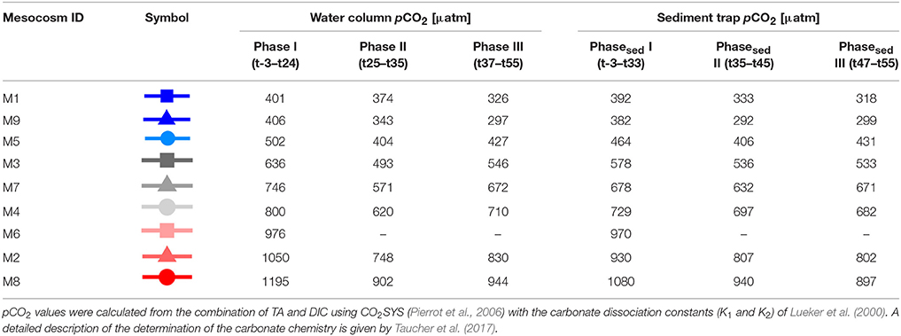
Table 1. Average values for seawater pCO₂ for each experimental phase, defined in section Chlorophyll a and Experimental Phases.

On October 23 (t22) approximately 85 m³ of deep-water were collected with a deep-water collecting system (described in detail by Taucher et al., 2017) from 650 m depth, approximately 7.5 km northeast of the study site. The collector was moored adjacent to the mesocosms. During the night between t23 and t24, approximately 20% of each mesocosms' volume was removed and replaced by equivalent amounts of nutrient-rich deep-water. Exact mixing ratios were calculated based on previously determined mesocosm volumes and target nutrient concentrations (Taucher et al., 2017). In total, the study lasted 61 days with the last sampling on t55 and t57 for the water column and sediment trap, respectively.

Alongside the regular sampling routine, we dedicated extensive effort to continuous maintenance of each mesocosm, including cleaning of the mesocosm walls. While divers regularly cleaned the outside, a cleaning ring was used to wipe the inside of the walls every week (Riebesell et al., 2013). This procedure prohibits wall growth, except for the flange ring connecting the mesocosm to the sediment trap and the funnel of the sediment trap, which are too narrow to be cleaned with the ring. Cleaning of these parts was thus performed by divers inside the mesocosms on t56, after the last sampling of the water column.

Sampling Procedure

Water Column

Samples were taken every second day between 9 a.m. and 12 p.m. We used two sampling systems simultaneously: (1) an integrating water sampler (IWS, HYDRO-BIOS, Kiel) for parameters that are sensitive to gas exchange or contamination and require low amounts of sample volume (e.g., carbonate chemistry) and (2) a vacuum pumping system for parameters that require large amounts of sample volume (e.g., particulate matter) (Taucher et al., 2017). Both systems allowed for integrated sampling of the entire water column of each mesocosm from 0 to 13 m water depth. All water column parameters presented in this study are thus given as integrated values for each mesocosm on the respective sampling day. Sampling was conducted every second day except for the time directly after deep-water addition (t25–t33), where samples were taken every day. Water collected with the pumping system was stored in 20 L carboys and transferred in a temperature-controlled room (set to in situ temperature) once they were transported back to the laboratory facilities. Carboys were always carefully mixed before withdrawing subsample volume in order to avoid sinking bias.

Additionally, net hauls were conducted on nine occasions during the 61 days experiment in order to estimate the abundance of mesozooplankton (e.g., copepods, appendicularians). Sampling frequency was restricted to one net haul every 4th sampling day in order to avoid overfishing. Samples were taken using an Apstein net (55 μm mesh size, 17 cm diameter opening) with a sampling volume of 295 L per haul. The net content was transferred into 500 mL Kautex bottles and immediately preserved with 4% formaldehyde buffered with sodium tetraborate solution until identification.

For the determination of microzooplankton abundances, 250 mL of unfiltered seawater was taken from the 20 L carboys and filled into brown glass bottles. Samples were preserved using acidic Lugol's solution (1–2% final concentration) and stored in the dark until enumeration with an inverse light microscope (section Zooplankton Counts).

Environmental boundary conditions [in situ temperature, salinity, pH, dissolved oxygen, chlorophyll a, and photosynthetically active radiation (PAR)] were monitored inside each mesocosm and in the surrounding seawater every sampling day using a hand-held self-logging CTD probe (CTD60M, Sea and Sun Technologies).

Sediment Trap

Sedimented POM was collected from each mesocosm every 48 h starting at t-3. Sampling was always carried out before the water column samples were taken to avoid re-suspension of sedimented matter. A detailed description of the sampling procedure is provided by Boxhammer et al. (2016). Briefly, sedimented material was pumped into 5 L Schott Duran glass bottles through the silicon tube connecting the collection cylinder of the sediment trap to the surface. All samples were collected within 0.5–1 h and immediately stored in large coolers filled with seawater and additional cool packs for the remaining sampling procedure to avoid warming and minimize bacterial degradation of the material. Once collection was finished, sediment trap samples were transported to the land-based facilities and processed as described in section POM in Sediment Trap Samples.

Sample Analysis

Chlorophyll a and Phytoplankton Pigments

Chlorophyll a and phytoplankton pigment concentrations were determined using reverse-phase high-performance liquid chromatography (HPLC). For this, we filtered up to 1.5 L of seawater onto glass fiber filters (nominal pore size of 0.7 μm, 25 mm diameter, Whatman) by gentle vacuum filtration (<200 mbar). During filtration, samples were covered with aluminum foil to reduce exposure to light. Pigments were extracted in acetone (90%) by homogenization of the filters with glass beads in a cell mill. Samples were then centrifuged (10 min, 5,200 rpm, 4°C) and the supernatant was filtered through 0.2 μm PTFE filters (VWR International). Pigment concentrations were determined in the supernatant by reverse-phase high-performance liquid chromatography (HPLC; Thermo Scientific HPLC Ultimate 3000 with an Eclipse XDB-C8 3.5 u 4.6 × 150 column; Van Heukelem and Thomas, 2001).

Contributions of individual phytoplankton groups to total chlorophyll a were then calculated using the software CHEMTAX (Mackey et al., 1996).

Zooplankton Counts

Mesozooplankton was analyzed quantitatively and taxonomically using a stereomicroscope (Olympus SZX9). Copepod abundances include copepodites as well as adults. Microzooplankton abundances were determined following the method described by Utermöhl (1931) using an inverted microscope (Zeiss Axiovert 25). Only the dominant groups of microzooplankton were counted, i.e., ciliates and heterotrophic dinoflagellates.

POM in Water Column Samples

For the determination of total particulate carbon (TPC), as well as particulate organic carbon, nitrogen and phosphorous (POC, PON, POP), we took up to 1 L subsample from the 20 L carboys. Subsamples were filtered with a gentle vacuum (<200 mbar) onto combusted glass fiber filters (nominal pore size of 0.7 μm, 25 mm diameter, Whatman). Filters for the determination of TPC were dried at 60°C over night and transferred into tin cups until analysis. Filters for POC and PON analysis were stored in combusted glass petri dishes at −20°C, while POP filters were directly transferred into 40 mL glass bottles and frozen at −20°C. POC,PON filters were fumed with hydrochloric acid (37%) for 2 h before measurement in order to remove particulate inorganic carbon (PIC). Concentrations of TPC, POC and PON were determined using an elemental CN analyser (EuroEA) following Sharp (1974).

POP filters were placed in 40 mL of deionized water with oxidizing decomposition reagent (“Oxisolve,” Merck) and autoclaved for 30 min in a pressure cooker to oxidize the particulate organic phosphorus to orthophosphate. After cooling, POP concentrations were determined by spectrophotometric analysis analogous to the method for dissolved inorganic phosphate, following Hansen and Koroleff (1999).

POM in Sediment Trap Samples

Quantities of the sediment trap material suspended in the 5 L bottles (see section Sediment Trap) were determined gravimetrically after transport to the laboratory. Afterwards, we homogenized the suspended material in the sampling bottles by gently mixing, to take subsamples for a variety of parameters, which are not considered any further in this study. Total subsample volume was small (generally <10% of bulk sample volume). The remaining bulk sample was transferred stepwise into 800 mL beakers and centrifuged therein with 5,236 × g for 10 min (6–16 KS centrifuge, SIGMA). The supernatant was then carefully decanted while the sedimented pellets were transferred into 110 mL centrifuge tubes. This procedure was repeated until the entire sample was centrifuged and transferred. For further compression, the 110 mL tubes were centrifuged a second time at 5,039 × g for 10 min (3K12 centrifuge, SIGMA) and the suspension was decanted. The remaining pellets were immediately deep frozen at −20°C and stored in small plastic screw cap cups. The centrifugation method was chosen over filtration since the latter only works with very small volumes of sedimented samples, due to the rapid clogging of the filter. A small sample volume of a rather patchy sample would then increase the error of later analyses for biogeochemical parameters. Concentrating the sample by centrifugation allows for an easier homogenization by grinding and thus reduces the error in later analyses.

The decanted supernatant was visually inspected for translucency and discarded unless there were still large amounts of organic material present in the supernatant. Between t35 and t49 we observed strongly elevated sedimentation and sample volumes increased drastically. During this period, translucency of the supernatant decreased as a larger proportion of the suspended matter could not be concentrated by centrifugation. We therefore pipetted small subsamples of the homogenized supernatant onto glass fiber filters (nominal pore size of 0.7 μm, 25 mm diameter, Whatman). All filters were deep-frozen at −20°C immediately after filtration for subsequent analysis of TPC, POC, PON, and POP as described for water column samples. In some cases the particle density of the original samples was too low for centrifugation to compress the sedimented matter into transferrable pellets (t21–t33 for M2 and t31–t33 for M8). In these cases we filtered subsamples of up to 100 mL for POM analysis of the entire samples as described for the supernatant at strongly elevated sedimentation.

The frozen centrifuge pellets were freeze-dried and ground to a very fine and homogenous powder as described in Boxhammer et al. (2016). This powder was then subsampled for the determination of TPC, POC, PON and POP. Duplicate subsamples of 2 mg were taken for the determination of TPC and transferred into tin cups. Additionally, two similar subsamples were transferred into silver cups and acidified before measurement to remove the inorganic carbon fraction (acidified for 1 h with 1M HCl and dried at 50°C over night). All four subsamples were measured using an elemental analyser (Euro EA–CN, Hekatech), which was calibrated with acetanilide (C₈H₉NO) and soil standard (Hekatech, catalog number HE33860101) prior to each measurement run. PIC was then calculated from total and organic carbon content. For the analysis of POP, subsamples of 2 mg were transferred into 40 mL glass vials and analyzed similar to the water column samples, as described above. In this study, sediment trap data are presented as daily fluxes, which we calculated by dividing the sediment trap data of each sampling point (every 48 h) by 2. Furthermore, the daily fluxes were normalized for mesocosm volume. Volume determination is described in the introductory paper to this special issue by Taucher et al. (2017).

Estimating Degradation of Sinking Particles Based on Stoichometry

Preferential remineralization of nitrogen and phosphorus over carbon is commonly observed in sinking POM, which leads to increasing elemental ratios (C:N, C:P) with depth (Sambrotto et al., 1993; Thomas et al., 1999; Schneider et al., 2003). We calculated the changes in elemental ratios between POM collected in the sediment trap and POM sampled from the water column and defined this ratio as the stoichiometry-based degradation index (SDI), as it gives an indication of the extent of degradation on sinking PM.

$\begin{array}{ll}{\mathit{\text{SDI}}}_{\text{C}\text{N}}={\text{C}:\text{N}}_{\text{s}\text{i}\text{n}\text{k}}/{\text{C}:\text{N}}_{\text{s}\text{u}\text{s}\text{p}}& (1)\end{array}$

$\begin{array}{ll}{\mathit{\text{SDI}}}_{\text{C}\text{P}}={\text{C}:\text{P}}_{\text{s}\text{i}\text{n}\text{k}}/{\text{C}:\text{P}}_{\text{s}\text{u}\text{s}\text{p}}& (2)\end{array}$

Here, a value of 1 indicates identical elemental ratios of POM suspended in the water column (e.g., C:N_susp) and POM collected in the sediment trap (e.g., C:N_sink), while values >1 denote higher C:N ratios in the sedimented POM compared to the water column, thus indicating preferential remineralization of nitrogen.

The SDI was calculated on a daily basis and does therefore not account for the time lag between POM production and sinking of POM to the sediment traps (Stange et al., 2017). The reason for this was that the time lag could only be accurately determined during the bloom, when clear peaks in biomass production and POM flux to the sediment traps were observed. It is, however, unlikely that a time lag of approximately 10 days, as observed between the peak of POM production in the water column and the peak of POM sedimentation, is the same for the entire experiment. We thus decided to calculate the SDI using the water column and sediment trap measurements of the same day. Nevertheless, calculating the SDI with a constant time lag of 10 days still resulted in similar trends and significant effects that were comparable to the ones reported in Table 3.

Data Analysis and Statistical Approach

To facilitate statistical analysis and a quantitative description of the data, we divided the dataset in three experimental phases based on the chlorophyll a development. A detailed description of the determination of the experimental phases is given in section Chlorophyll a and Experimental Phases. We applied linear regression analysis to determine the relationship between average pCO₂ and average response of the variables during each phase. The model results were checked for normality and homoscedasticity. A linear regression was performed for several reasons. First of all, a non-linear analysis requires an underlying hypothesis of a non-linear relationship between predictor and response variable. Since there was no physiological reason to suspect a non-linear relationship, a linear model is more conservative and prevents the risk of overfitting. Furthermore, our analyses did not aim to identify a certain pCO₂ level as a tipping point, but rather aimed to verify whether there is an overall effect. Cases where a non-linear relation may be underlying are discussed as such in the text. Unfortunately, Mesocosm 6 was irreparably damaged on t26 and thus excluded from the statistical analysis of phases II and III. Statistical analyses were undertaken using the software R, version 3.3.1 (R Core Team, 2013).

Results

Chlorophyll a and Experimental Phases

The experiment started in oligotrophic conditions, with very low concentrations of inorganic nutrients (Figure S5) and chlorophyll a (Figure 1A). Chlorophyll a concentration during phase I (t-3–t24) averaged at approximately 0.1 μg L⁻¹. On t24 we added nutrient-rich deep-water to the mesocosms in order to simulate an eddy-induced upwelling event (for a detailed description of the deep-water addition see Taucher et al., 2017). The deep-water addition increased inorganic nutrient concentrations to approximately 3.15, 0.17, and 1.60 μmol L⁻¹ for ${\text{NO}}_3^{-}+$${\text{NO}}_2^{-}$, ${\text{PO}}_4^{3-}$, and Si(OH)₄, respectively. This stimulated the rapid development of a phytoplankton bloom in phase II (t25–t35) with a peak in chlorophyll a at t28 (Figure 1). The inorganic nutrients were quickly depleted and reached values close to detection limit between t28 and t30 (Figure S5). After the peak on t28 chlorophyll a concentrations decreased rapidly in all mesocosms until they reached a minimum at t35. In the post-bloom phase (phase III, t37–t55) inorganic nutrients and chlorophyll a concentrations remained low, except for the two mesocosms with highest CO₂, which displayed elevated chlorophyll a until the end of the experiment. Experimental phases were defined differently for the POM flux to the sediment traps, as described in section Sediment Trap. We further observed a well-mixed water column regarding the in situ temperature and salinity throughout the experiment (Taucher et al., 2017).

FIGURE 1

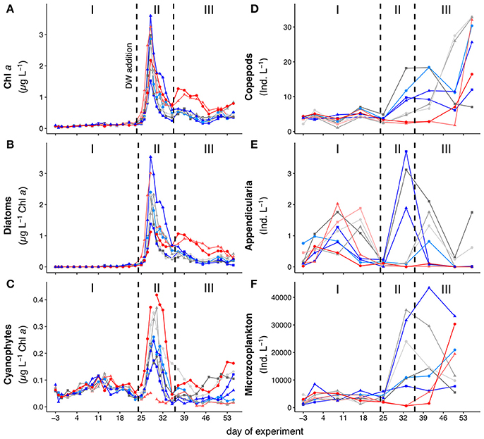
Figure 1. Development of (A) chlorophyll a concentrations. (B) Abundances of diatoms, and (C) abundances of cyanophytes. (D–F) depict zooplankton abundances over the course of the experiment with (B) copepods, including both adult and all copepodite stages, (C) appendicularians, and (D) protozoan microzooplankton, mostly ciliates and heterotrophic dinoflagellates. The three different phases are indicated with I, II and III and separated by the dashed vertical lines. Note that the first dashed line also depicts the time of deep-water addition. Colors and symbols are described in Table 1.

Temporal Dynamics in Plankton Community Composition

Figures 1B,C shows the development of cyanophytes and diatoms over the course of the experiment. We only focused on these groups since they had by far the largest contribution to total chlorophyll a concentrations during the respective experimental phases. During the oligotrophic phase I, (pico-)cyanobacteria (Synechococcus sp.) were the dominant phytoplankton group, with a contribution of 70–80% to total chlorophyll a (Figures S1A,B). Abundances of this group increased toward t11 and decreased afterwards until the deep-water addition on t24. We observed a significant positive effect of pCO₂ on the abundance of cyanophytes during phase I (p = 0.002, F = 26.67).

Following the deep-water addition on t24, the phytoplankton community underwent significant changes. Throughout phases II and III, large chain-forming diatoms, such as Leptocylindrus sp., Guinardia sp., and Bacteriastrum sp. dominated the phytoplankton community with a contribution to total chlorophyll a concentrations of 50–70% (Figure S1B). While their overall abundance decreased toward the end of the experiment, diatoms were still the dominant phytoplankton group throughout phase III. This dominance was particularly pronounced in both high CO₂ mesocosms (M2 and M8, see Figure 1B) and we observed a significant positive effect of pCO₂ on the abundance of diatoms during phase III (p = 0.026, F = 8.71). Plankton community structure and species succession during this study closely resembled those during natural bloom events in the Canary Islands region (Basterretxea and Arístegui, 2000; Arístegui et al., 2004) and are thus representative for natural marine ecosystems of the study area.

Figures 1B–D shows the temporal development of micro- and mesozooplankton abundances in all mesocosms. For the purpose of this study, we only differentiated between copepods, appendicularians and microzooplankton. Abundances of copepods were constantly low throughout phase I of the experiment. Appendicularian abundances increased during phase I in all mesocosms, but declined again and reached a minimum right after deep-water addition. Phase II and III were characterized by higher abundances of both groups in all mesocosms, except in M2 and M8. While abundances of appendicularians in those two mesocosms remained low until the end of the experiment, copepod abundances increased from t50 to the last sampling day. Microzooplankton abundances were overall low during phase I of the experiment and started to increase in all mesocosms after t25, but remained comparably low in M2 and M8.

Temporal Dynamics of POM

Water Column

The temporal development of POC, PON, and POP in the water column is shown in Figures 2A–C. Water column POC and PON concentrations were only determined from t9 onwards as we did not have sufficient filtration volume during the first couple of days. Concentrations of all three parameters remained low from t9 onwards, but increased slightly toward the end of phase I (t17–t23). With the addition of deep-water at t24, POM increased rapidly in the water column and peaked between t30 and t31 in all mesocosms. After the peak in phase II, most POM was retained in the water column and only slowly decreased during phase III. We observed a slight but significant negative effect of pCO₂ on POP during phase I (Table 2), but this effect vanished during the subsequent phases. During phase III, concentrations of water column POC, PON and POP were elevated in the two highest CO₂ mesocosms (M2 and M8), but we did not detect an overall significant effect of pCO₂.

FIGURE 2

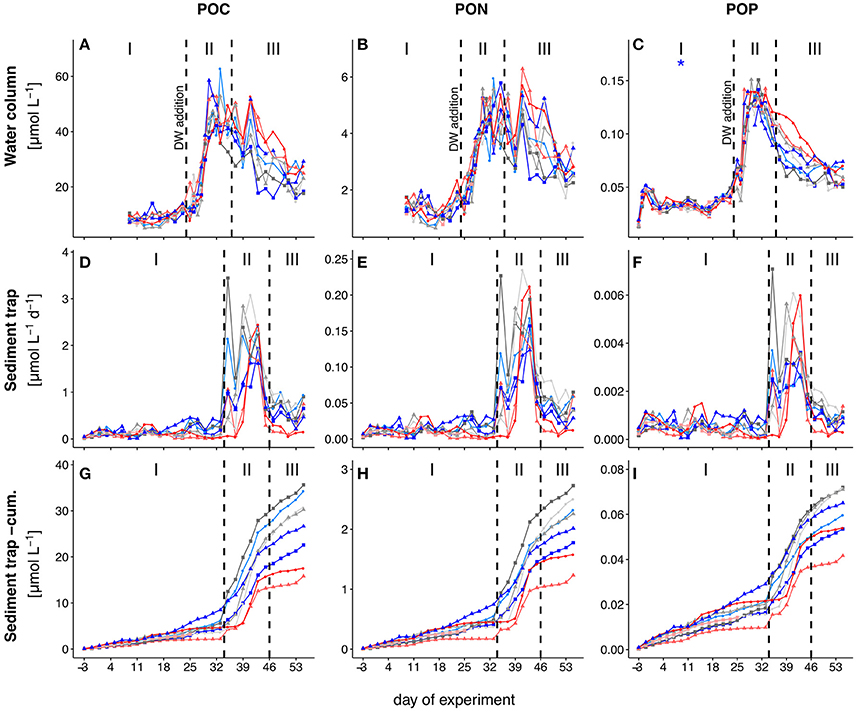
Figure 2. Temporal development of standing stocks and fluxes of total particulate carbon (TPC; A,D,G), nitrogen (TPN; B,E,H) and phosphorus (TPP; C,F,I). (A–C) and (D–F) depict POM concentrations from the water column and daily flux to the sediment trap, respectively. (G–I) show the cumulative flux of POM to the sediment trap. Colored lines depict the different mesocosms. The three different phases are indicated with I, II, and III and separated by the dashed vertical lines. Note that the first dashed line in (A–C) also depicts the time of deep-water addition. Colors and symbols are described in Table 1. The * denotes a statistically significant postitive (red) or negative (blue) effect of CO₂ during the respective experimental phase.

TABLE 2

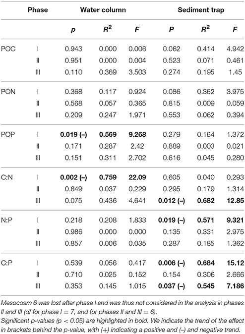
Table 2. Statistical results from the linear regression analysis on response means over the respective phases.

Sediment Trap

Peaks in POM sedimentation were temporally delayed to POM concentration peaks in the water column. This temporal delay can be explained by particle aggregation dynamics, as the rapid growth rate of phytoplankton due to the pulsed nutrient addition first resulted in an increasing abundance of smaller particles. The POM formed in the water column thus only started to sink after larger aggregates had formed several days after the peak in the water column (Taucher et al., in review). Due to this delay, and in order to correctly compare water column and sedimented POM, we define experimental phases differently for the sediment trap material (phase_sed I = t-3–t33; phase_sed II = t35–t45; phase_sed III = t47–t55). While this approach does not take into account the influence of changes in sinking velocity of sedimenting particles on the time lag between OM production in the water column and its sedimentation to the sediment trap, we argue that in this experiment differences in aggregation dynamics were the main driver of this delay.

Total POM fluxes to the sediment trap were low throughout phase_sed I (Figures 2D–F). The onset of increased POM fluxes to the sediment trap followed water column POM build-up with a temporal delay of approximately 10 days. After an initial peak in POM flux on t35 (phase_sed II), we observed rather low sedimentation rates on t37. This changed again on t39, after which sedimentation rates stayed high until t43. M3 and M5 had the largest contribution to the initial peak on t35, while the remaining mesocosms showed highest sedimentation rates on t39 and t43. Rates decreased during the last phase_sed (t45 to t55) but were still higher than in phase_sed I. The two mesocosms with highest CO₂ concentrations (M2, M8) showed particularly low sedimentation rates during phase_sed III. However, we did not detect a significant effect of pCO₂ in the regression analysis (Table 2).

The analysis of filters taken due to low translucency of the supernatant during the period of high sedimentation (t35–t49; described in section POM in Sediment Trap Samples) contributed generally less than 4% to the total concentration of the respective parameter and was thus neglected. The cleaning of the lowest segment of the mesocosms and sediment trap walls on the last day of the experiment (day 57) resulted in strongly elevated sedimentation rates since there was considerable growth of benthic autotrophs on this segment (Figure S2). We thus excluded this day from the analysis.

Dynamics in Elemental Stoichiometry

Water Column

We observed higher ratios of C:N (POC:PON), N:P (PON:POP), and C:P (POC:POP) compared to Redfield proportions (C:N:P = 106:16:1) throughout almost the entire experiment (Figures 3A–C). The only exceptions were C:N ratios during phase I (t9–t13) and during the phytoplankton bloom right after the addition of deep-water (t25–t28). We observed a small peak in C:N stoichiometry between t17 and t19 in all mesocosms. C:N ratios subsequently declined until the deep-water addition and fluctuated close to Redfield proportions of approximately 6–7 from t25–t28. C:N ratios increased profoundly directly after the bloom peak and nutrient depletion (t29 until t32). After this transient peak, C:N decreased toward the end of the experiment. Statistical analysis of C:N ratios averaged over the entire experiment did not reveal a significant effect of pCO₂. However, when we tested each phase individually, we observed a significantly negative effect of pCO₂ on C:N during phase I (see Table 2). We also found a borderline insignificant positive effect on C:N during phase III. However, the lack of significance was likely due to the effect being exclusively driven by both high CO₂ mesocosms instead of a linear relationship (see Figure S3C).

FIGURE 3

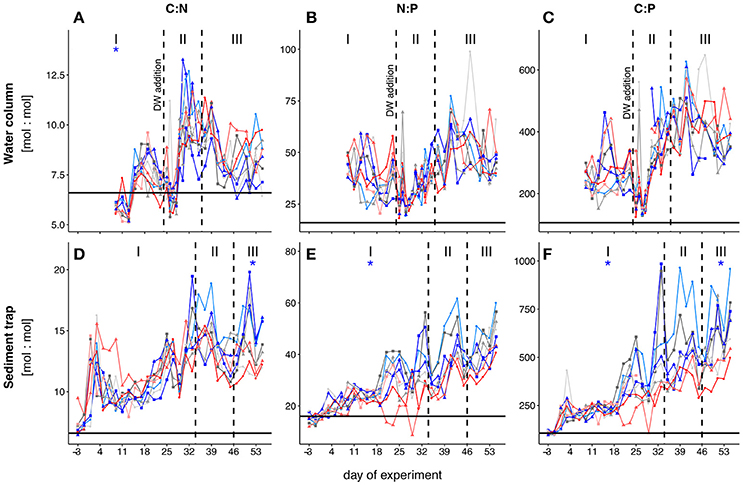
Figure 3. Temporal development of POM elemental stoichiometries in the water column (A–C) and the sediment trap samples (D–F). Black horizontal lines indicate Redfield proportions for the respective elemental ratios (C:N = 6.6, N:P = 16, C:P = 106). Colored lines depict the different mesocosms. The three different phases are indicated with I, II and III and separated by the dashed vertical lines. Note that the phases for water column and sediment trap POM have been defined differently (see section Chlorophyll a and Experimental Phases). Colors and symbols are described in Table 1. The * denotes a statistically significant postitive (red) or negative (blue) effect of CO₂ during the respective experimental phase.

Both N:P and C:P did not show a clear change during phase I. Similar to C:N, we observed minimum values for both ratios right after deep-water addition. While C:P also increased rapidly after t28 and stayed constant afterwards, N:P was characterized by a comparably slow and steady increase toward the end of the experiment. We neither observed significant treatment effects on C:P and N:P when averaged over the entire time, nor for any of the three phases individually.

Sediment Trap

C:N and C:P ratios of sediment trap material were above Redfield and also higher than in water column POM (Figures 3D,F). This difference was less pronounced in the N:P ratios (Figure 3E). We observed a slow and steady increase in all ratios over the course of the experiment. After t19, the variability between mesocosms increased in N:P and C:P and stayed high until the end of the experiment. We observed a significant negative effect of pCO₂ on the C:N ratio in sedimented POM during phase_sed III (see Table 2) as well as on N:P during phase_sed I and C:P during phases_sed I and III. These CO₂ effects were driven primarily by the very low values in the two highest CO₂ mesocosms (M2 and M8) (Figures 3D–F).

Temporal Development of the SDI

SDI_CN was above 1 in all mesocosms throughout the experiment, with only few exceptions (see Figure 4A). This shows that C:N ratios in the sediment trap were higher compared to those in the water column for most of the time. There was no clear trend of SDI_CN over time, however, the ratio fluctuated in all mesocosms from the beginning up until t39 and stayed more or less constant after that. We observed a significant positive treatment effect of CO₂ on SDI_CN during phase I and a highly significant negative treatment effect during phase III (see Table 3).

FIGURE 4

Figure 4. SDI (stoichiometry-based degradation index), depicting the relation between the elemental stoichiometries of the water column and sedimented POM. SDI of C:N (A) and C:P (B). The horizontal lines indicate a 1:1 relationship and thus equal stoichiometries in the sediment trap and water column POM. The dashed vertical lines indicate experimental phases for water column material. Colors and symbols are described in Table 1. The * denotes a statistically significant postitive (red) or negative (blue) effect of CO₂ during the respective experimental phase.

TABLE 3

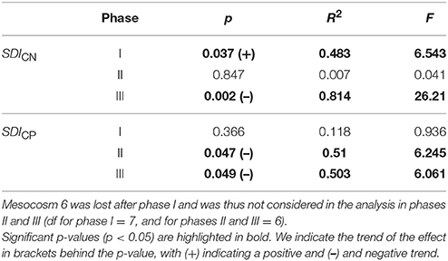
Table 3. Statistical results from the linear regression analysis on response means over the respective phases.

SDI_CP did not strongly deviate from one during the majority of phase I except for the first two sampling days (Figure 4B). SDI_CP increased during phase II and remained elevated throughout phase III except for mesocosms M4, M2 and M8. We observed significant negative CO₂ treatment effects on SDI_CP during phases II and III.

Discussion

Temporal Development of POM Standing Stocks

CO₂-related differences in standing stocks and elemental composition of POM were detected primarily after the phytoplankton bloom in phase II and more pronounced during phase III (Figures 2, 3). In particular, we observed that in both mesocosms with highest pCO₂, post-bloom water column POM remained at high concentrations longer than in low and intermediate treatment levels. This led to less sedimentation of POC, PON, and POP to the sediment trap during the study period under high pCO₂ (see the cumulative plots of sedimented matter in Figures 2G–I). However, the CO₂ trend was not linear, but driven almost entirely by the two mesocosms with highest pCO₂ (M2 and M8, Figures S3A,B). There are three possible explanations for the observed differences in post-bloom water column POM retention: Differences in (1) particle load with ballasting minerals, such as calcite, opal or lithogenic material, (2) grazing and thus repackaging by micro- and mesozooplankton, or (3) the rate of sinking particle formation (aggregation rate).

PIC/POC and biogenic silica (BSi)/POC ratios (Figure S4) did not give an indication for a lower ballasting effect in mesocosms M2 and M8 after the bloom and we have no reason to expect a differing supply of airborne lithogenic material to individual mesocosms. We thus conclude that the difference in POM retention was most likely driven by differences in food-web dynamics and/or aggregation processes. Indeed, abundances of the dominant groups of mesozooplankton, i.e., copepods and appendicularians, as well as microzooplankton abundances were particularly low in both high CO₂ mesocosms during phases II and III (Figures 1D–F). Although the difference in grazer abundance was mainly driven by M2 and M8, the linear regression analysis revealed significantly lower abundances of copepods on t41 with increasing pCO₂ (F = 5.469, p = 0.05). These results are further supported by the results of the multivariate analysis using Bray–Curtis dissimilarity, which showed that M2 and M8 were particularely different to the other mesocosms in terms of their plankton community composition (Taucher et al., 2017). The lower abundance of grazers in the highest CO₂ treatment levels may have resulted in reduced consumption and repackaging of POM, which in turn translated into a longer residence time of phytoplankton cells and aggregates in the water column. On the other hand, the comparatively high abundances of zooplankton grazers in the other mesocosms resulted in higher clearance rates of approximately 9 L d⁻¹ (assuming an a mean abundance of 10 ind. L⁻¹ with an average body size of less than 500 μm; Kiørboe, 2011), which further illustrates the strong influence of zooplankton grazing on controlling and modifying the elemental flux to the sediment traps.

The increased retention of water column POM in M2 and M8 may also be explained by lower aggregation rates. While possibly lower turbulence inside the mesocosms compared to the surrounding water column may result in overall lower aggregation rates, the similarly mixed water columns did not suggest strong differences in turbulence between the individual mesocosms. This suggests that other processes were the key drivers of the difference in OM retention in the water column. Differences in phytoplankton community composition, nutritional status and growth phase of the cells can profoundly influence the coagulation efficiency (Kiørboe et al., 1990; Kiørboe and Hansen, 1993; Burd and Jackson, 2009). However, measurements of the in situ particle size spectrum by Taucher et al. (in review) did not reveal CO₂ related differences for the start and rate of aggregate formation. We thus conclude that the increased retention of water column POM under elevated CO₂ is primarily driven by differences in zooplankton abundance.

Temporal Development of Element Stoichiometry

Elemental ratios in water column POM were much higher than Redfield values for the majority of time during the experiment. This deviation is likely caused by very low concentrations of all major inorganic nutrients. Exceptions to this trend were observed in water column C:N ratios, which were substantially lower in the middle of phase I and right before the deep-water addition. We observed a small bloom of cyanophytes (mainly Synechococcus sp.) during phase I, with a peak in abundances around t11 (Figure 1C). While nutrient concentrations were generally low throughout phase I (mean concentrations of ${\text{NO}}_3^{-}$ + ${\text{NO}}_2^{-}$ = 0.05 μmol L⁻¹ and ${\text{PO}}_4^{3-}$ = 0.03 μmol L⁻¹; Figure S5), excess phosphate was available during phase I (mean ${\text{NO}}_3^{-}+$${\text{NO}}_2^{-}$/${\text{PO}}_4^{3-}$ = 2). Synechococcus has been shown to have particularly low intercellular C:N ratios during exponential growth (Bertilsson et al., 2003). Since this group dominated the phytoplankton community during phase I, it is likely that their C:N signature is reflected in the C:N ratios of water column POM. The small bloom of cyanophytes collapsed after t11 and water column C:N increased correspondingly in the following days. During this period, we observed a significantly negative effect of pCO₂ on water column C:N ratios (Figure 3A). This effect again correlates well with the significantly higher abundances of cyanobacteria observed under elevated levels of CO₂ during that phase.

With the addition of deep-water on t24, inorganic nutrient limitation was relieved for about 4 days. Consequently, C:N and C:P ratios of water column POM declined immediately after the addition on t24 and stayed low until t28 (Figures 3A,C). C:N and C:P increased rapidly back to elevated values as soon as inorganic nutrients from deep-water addition were depleted. This indicates carbon overconsumption, a mechanism observed in many groups of marine phytoplankton, particularly in diatoms, under nutrient-deplete conditions (Toggweiler, 1993; Riebesell et al., 2007). Indeed, diatoms were the dominant phytoplankton group during the bloom in all mesocosms, with a contribution of >60% to the total chlorophyll a concentrations (Taucher et al., 2017). Additionally, the overall low N:P ratios throughout the experiment suggests that the community was mainly phosphate-limited throughout the experiment (Figure 3B).

We observed a borderline insignificant effect (p = 0.075) of pCO₂ on the elemental stoichiometry of water column POM during phase III of the experiment. We argue that our analysis did not reveal a significant effect as the difference in C:N wasn't linear, but solely driven by both mesocosms with highest pCO₂ (Figure S3C). This difference is likely caused by differences in phytoplankton community composition. Abundances of large diatoms were significantly increased in both mesocosms with highest pCO₂ during phase III (Figure 1B) and they continued to increase even after the supplied nutrients were depleted on t28. The difference in abundance thus likely increased the magnitude of carbon overconsumption in the two highest CO₂ treatments, resulting in slightly higher C:N ratios in M2 and M8.

Influence of Community Structure on the Degradation of Sinking POM

SDI_CN and SDI_CP were larger than 1 for the majority of the experiment. This shows that elemental ratios of sedimented POM were overall elevated compared to those of POM suspended in the water column. A similar trend has also been observed to a lesser degree in a previous study (Czerny et al., 2013), and was interpreted as an indication for preferential remineralization of both N and P relative to C in sinking organic material (Sambrotto et al., 1993; Thomas et al., 1999; Schneider et al., 2003).

We observed a significant positive effect of pCO₂ on SDI_CN during phase I, suggesting that degradation processes were more pronounced under high CO₂ before the deep-water addition. This trend reversed during and after the bloom and a significant negative effect of pCO₂ was detected for SDI_CP during phase II and SDI_CN and SDI_CP during phase III. In order to identify the mechanisms responsible for the observed differences, we evaluated the processes, which have the potential to alter C:N and C:P stoichiometry in sinking POM. These include the degradation of POM by grazers (protozoans and metazoans) and bacteria.

Zooplankton grazers are known to assimilate nitrogen and phosphorus more efficiently than carbon in order to maintain homeostasis, i.e., keeping their elemental composition constant (Checkley and Entzeroth, 1985; Daly et al., 1999). The excess carbon is either respired, internally stored in lipid reservoirs (e.g., in overwintering copepods in the Arctic), or defecated, resulting in fecal pellets with substantially higher C:N ratios than sinking aggregates or marine phytoplankton (Gerber and Gerber, 1979; Small et al., 1983; Daly et al., 1999). Another pathway that has the potential to impact the stoichiometry of sinking POM is bacterial degradation. It has been shown that the rapid decrease of sinking particulate matter with depth is partly associated with degradation processes by particle-attached bacteria (Smith et al., 1992; Ploug and Grossart, 2000). However, production rates of free-living and particle-associated bacteria were not significantly different in the high CO₂ treatments throughout the experiment (Hornick, unpublished data). Furthermore, CO₂-related differences in zooplankton abundances between mesocosms only manifested during phase II and III (see Figure 1). We can therefore only speculate that the higher SDI_CN under elevated levels of CO₂ during phase I is most likely related to differences in the quality of the sinking POM. Contrastingly, the significant negative effects of pCO₂ on SDI_CN and SDI_CP during phase II and III are indicative for slower degradation of sinking organic material, which correlates well with the lower abundances of micro- and mesozooplankton during these periods.

In an earlier study by Riebesell et al. (2007), increased consumption of dissolved inorganic carbon (DIC) with increasing levels of seawater pCO₂ was observed in an enclosed natural plankton community. The authors extrapolated these results and argued that this increased consumption may translate to enhanced carbon relative to nitrogen drawdown from the euphotic zone. In this study, we also observed slightly higher C:N ratios in water column POM in both mesocosms with highest pCO₂ (Figure 3A), indicating that elevated levels of CO₂ may indeed promote carbon overconsumption. However, our results show that the degradation by micro- and mesozooplankton tightly controlled the fate of POM stoichiometry with depth, with the possibility to reverse CO₂ trends in elemental stoichiometry observed in the surface. We thus argue that changes in the elemental stoichiometry of suspended POM in the surface cannot be extrapolated to depth without estimating the degradation processes, which in turn are controlled by the plankton community structure.

Conclusion

In the present study, we show that OA induced changes in plankton community structure can significantly influence the degradation of sinking POM. We found that C:N ratios in suspended POM were slightly elevated after a diatom-dominated phytoplankton bloom in the two mesocosms with highest pCO₂, most likely due to enhanced carbon overconsumption. Yet, POM collected in the sediment traps showed significantly lower C:N ratios under high CO₂ conditions. This indicates that degradation of sinking matter was less pronounced under elevated levels of CO₂, which we mainly attribute to the lower abundances of micro- and mesozooplankton in those mesocosms during and after the phytoplankton bloom. These trends only manifested during post-bloom conditions, 4 weeks into the experiment, when differences in community structure were most pronounced. Our findings underline that CO₂ induced changes in elemental stoichiometry of sinking POM are ultimately controlled by the plankton community structure. In particular, our results highlight the importance of micro- and mesozooplankton grazers on the transformation of sinking organic matter and we suggest that extrapolations of biogeochemical processes to global scales cannot be made without considering the entire planktonic food web.

Author Contributions

UR, JT, LB, TB, and PS: contributed to the design of the study; LK, TB, and PS: analyzed sediment trap samples; MA-M and HH: analyzed the zooplankton samples; AN: analyzed the water column samples; PS interpreted the data and wrote the manuscript with comments from all co-authors.

Funding

This project was funded by the German Federal Ministry of Education and Research (BMBF) in the framework of the coordinated project BIOACID—Biological Impacts of Ocean Acidification, phase 2 (FKZ 03F06550). UR received additional funding from the Leibniz Award 2012 by the German Research Foundation (DFG).

Conflict of Interest Statement

The authors declare that the research was conducted in the absence of any commercial or financial relationships that could be construed as a potential conflict of interest.

Acknowledgments

The authors of this paper are very thankful to the entire Gran Canaria KOSMOS consortium for their contribution to this experiment. We also would like to thank the Oceanic Platform of the Canary Islands (Plataforma Oceánica de Canarias, PLOCAN) for sharing their expertise and research facilities, and providing us with all the necessary tools to successfully conduct our research. Another special thanks goes to the Marine Science and Technology Park (Parque Científico Tecnológico Marino, PCTM) and the Spanish Bank of Algae (Banco Español de Algas, BEA), both from the University of Las Palmas (ULPGC), who provided additional facilities to run experiments, measurements, and analyses.

We are also thankful for the great support by the captain and crew of RV Hesperides for deploying and recovering the mesocosms (cruise 29HE20140924), and RV Poseidon for transporting the mesocosms and their support in testing the deep water collector during cruise POS463.

Supplementary Material

The Supplementary Material for this article can be found online at: https://www.frontiersin.org/articles/10.3389/fmars.2018.00140/full#supplementary-material

References

Arístegui, J., Barton, E. D., Tett, P., Montero, M. F., García-Muñoz, M., Basterretxea, G., et al. (2004). Variability in plankton community structure, metabolism, and vertical carbon fluxes along an upwelling filament (Cape Juby, NW Africa). Prog. Oceanogr. 62, 95–113. doi: 10.1016/j.pocean.2004.07.004

CrossRef Full Text | Google Scholar

Arístegui, J., Hernández-León, S., Montero, M. F., and Gómez, M. (2001). The seasonal planktonic cycle in coastal waters of the Canary Islands. Sci. Mar. 65, 51–58. doi: 10.3989/scimar.2001.65s151

CrossRef Full Text | Google Scholar

Bach, L. T., Taucher, J., Boxhammer, T., Ludwig, A., Achterberg, E. P., Algueró-Muñiz, M., et al. (2016). Influence of Ocean acidification on a natural winter-to-summer plankton succession: first insights from a long-term mesocosm study draw attention to periods of low nutrient concentrations. PLoS ONE 11:e0159068. doi: 10.1371/journal.pone.0159068

PubMed Abstract | CrossRef Full Text | Google Scholar

Basterretxea, G., and Arístegui, J. (2000). Mesoscale variability in phytoplankton biomass distribution and photosynthetic parameters in the Canary-NW African coastal transition zone. Mar. Ecol. Prog. Ser. 197, 27–40. doi: 10.3354/meps197027

CrossRef Full Text | Google Scholar

Bertilsson, S., Berglund, O., Karl, D. M., and Chisholm, S. W. (2003). Elemental composition of marine Prochlorococcus and Synechococcus : implications for the ecological stoichiometry of the sea. Limnol. Oceanogr. 48, 1721–1731. doi: 10.4319/lo.2003.48.5.1721

CrossRef Full Text | Google Scholar

Boxhammer, T., Bach, L. T., Czerny, J., and Riebesell, U. (2016). Technical note: sampling and processing of mesocosm sediment trap material for quantitative biogeochemical analysis. Biogeosciences 13, 2849–2858. doi: 10.5194/bg-13-2849-2016

CrossRef Full Text | Google Scholar

Burd, A. B., and Jackson, G. A. (2009). Particle aggregation. Ann. Rev. Mar. Sci. 1, 65–90. doi: 10.1146/annurev.marine.010908.163904

PubMed Abstract | CrossRef Full Text | Google Scholar

Caldeira, K., and Wickett, M. E. (2003). Oceanography: anthropogenic carbon and ocean pH. Nature 425:365. doi: 10.1038/425365a

CrossRef Full Text | Google Scholar

Checkley, D. M., and Entzeroth, L. C. (1985). Elemental and isotopic fractionation of carbon and nitrogen by marine, planktonic copepods and implications to the marine nitrogen cycle. J. Plankton Res. 7, 553–568. doi: 10.1093/plankt/7.4.553

CrossRef Full Text | Google Scholar

Czerny, J., Schulz, K. G., Boxhammer, T., Bellerby, R. G. J., Büdenbender, J., Engel, A., et al. (2013). Implications of elevated CO₂ on pelagic carbon fluxes in an Arctic mesocosm study - an elemental mass balance approach. Biogeosciences 10, 3109–3125. doi: 10.5194/bg-10-3109-2013

CrossRef Full Text | Google Scholar

Daly, K. L., Wallace, D. W. R., Smith, W. O., Skoog, A., Lara, R., Gosselin, M., et al. (1999). Non-Redfield carbon and nitrogen cycling in the Arctic: effects of ecosystem structure and dynamics. J. Geophys. Res. Ocean. 104, 3185–3199. doi: 10.1029/1998JC900071

CrossRef Full Text | Google Scholar

Doney, S. C., Fabry, V. J., Feely, R. A., and Kleypas, J. A. (2009). Ocean acidification: the other CO₂ problem. Ann. Rev. Mar. Sci. 1, 169–192. doi: 10.1146/annurev.marine.010908.163834

PubMed Abstract | CrossRef Full Text | Google Scholar

Fabricius, K. E., Langdon, C., Uthicke, S., Humphrey, C., Noonan, S., De'ath, G., et al. (2011). Losers and winners in coral reefs acclimatized to elevated carbon dioxide concentrations. Nat. Clim. Chang. 1, 165–169. doi: 10.1038/nclimate1122

CrossRef Full Text | Google Scholar

Gazeau, F., Sallon, A., Maugendre, L., Louis, J., Dellisanti, W., Gaubert, M., et al. (2016). First mesocosm experiments to study the impacts of ocean acidification on plankton communities in the NW Mediterranean Sea (MedSeA project). Estuar. Coast. Shelf Sci. 138, 11–29. doi: 10.1016/j.ecss.2016.05.014

CrossRef Full Text | Google Scholar

Gerber, R. P., and Gerber, M. B. (1979). Ingestion of natural particulate organic matter and subsequent assimilation, respiration and growth by tropical lagoon zooplankton. Mar. Biol. 52, 33–43. doi: 10.1007/BF00386855

CrossRef Full Text | Google Scholar

Hall-Spencer, J. M., Rodolfo-Metalpa, R., Martin, S., Ransome, E., Fine, M., Turner, S. M., et al. (2008). Volcanic carbon dioxide vents show ecosystem effects of ocean acidification. Nature 454, 96–99. doi: 10.1038/nature07051

PubMed Abstract | CrossRef Full Text | Google Scholar

Hansen, H. P., and Koroleff, F. (1999). “Determination of nutrients,” in Methods of Seawater Analysis, eds K. Grasshoff, K. Kremling, and M. Ehrhardt (Weinheim: Wiley-VCH Verlag GmbH), 159–228.

IPCC (2014). “Technical summary,” in Climate Change 2013 - The Physical Science Basis, ed Intergovernmental Panel on Climate Change (Cambridge: Cambridge University Press), 31–116.

Kiørboe, T. (2011). How zooplankton feed: mechanisms, traits and trade-offs. Biol. Rev. 86, 311–339. doi: 10.1111/j.1469-185X.2010.00148.x

PubMed Abstract | CrossRef Full Text | Google Scholar

Kiørboe, T., and Hansen, J. L. S. (1993). Phytoplankton aggregate formation: observations of patterns and mechanisms of cell sticking and the significance of exopolymeric material. J. Plankton Res. 15, 993–1018. doi: 10.1093/plankt/15.9.993

CrossRef Full Text | Google Scholar

Kiørboe, T., Andersen, K. P., and Dam, H. G. (1990). Coagulation efficiency and aggregate formation in marine phytoplankton. Mar. Biol. 107, 235–245. doi: 10.1007/BF01319822

CrossRef Full Text | Google Scholar

Le Quéré, C., Andrew, R. M., Canadell, J. G., Sitch, S., Korsbakken, J. I., Peters, G. P., et al. (2016). Global Carbon Budget 2016. Earth Syst. Sci. Data 8, 605–649. doi: 10.5194/essd-8-605–2016.

CrossRef Full Text | Google Scholar

Lueker, T. J., Dickson, A. G., and Keeling, C. D. (2000). Ocean pCO₂ calculated from dissolved inorganic carbon, alkalinity, and equations for K1 and K2: validation based on laboratory measurements of CO₂ in gas and seawater at equilibrium. Mar. Chem. 70, 105–119. doi: 10.1016/S0304-4203(00)00022-0

CrossRef Full Text | Google Scholar

Mackey, M., Mackey, D., Higgins, H., and Wright, S. (1996). CHEMTAX - a program for estimating class abundances from chemical markers:application to HPLC measurements of phytoplankton. Mar. Ecol. Prog. Ser. 144, 265–283. doi: 10.3354/meps144265

CrossRef Full Text | Google Scholar

Orr, J. C., Fabry, V. J., Aumont, O., Bopp, L., Doney, S. C., Feely, R. A., et al. (2005). Anthropogenic ocean acidification over the twenty-first century and its impact on calcifying organisms. Nature 437, 681–686. doi: 10.1038/nature04095

PubMed Abstract | CrossRef Full Text | Google Scholar

Oschlies, A., Schulz, K. G., Riebesell, U., and Schmittner, A. (2008). Simulated 21st century's increase in oceanic suboxia by CO₂-enhanced biotic carbon export. Global Biogeochem. Cycles 22:GB4008. doi: 10.1029/2007GB003147

CrossRef Full Text | Google Scholar

Paul, A. J., Bach, L. T., Schulz, K. G., Boxhammer, T., Czerny, J., Achterberg, E. P., et al. (2015). Effect of elevated CO₂ on organic matter pools and fluxes in a summer Baltic Sea plankton community. Biogeosciences 12, 6181–6203. doi: 10.5194/bg-12-6181-2015

CrossRef Full Text | Google Scholar

Pierrot, D., Lewis, E., and Wallace, D. W. R. (2006). MS Excel Program Developed for CO₂ System Calculations. ORNL/CDIAC-105a.

Ploug, H., and Grossart, H.-P. (2000). Bacterial growth and grazing on diatom aggregates: respiratory carbon turnover as a function of aggregate size and sinking velocity. Limnol. Oceanogr. 45, 1467–1475. doi: 10.4319/lo.2000.45.7.1467

CrossRef Full Text | Google Scholar

R Core Team (2013). R: A Language and Environment for Statistical Computing.

Riebesell, U., and Gattuso, J. (2015). Lessons learned from ocean acidification research. Nat. Publ. Gr. 5, 12–14. doi: 10.1038/nclimate2456

CrossRef Full Text | Google Scholar

Riebesell, U., Bach, L. T., Bellerby, R. G. J., Monsalve, J. R. B., Boxhammer, T., Czerny, J., et al. (2017). Competitive fitness of a predominant pelagic calcifier impaired by ocean acidification. Nat. Geosci. 10, 19–23. doi: 10.1038/ngeo2854

CrossRef Full Text | Google Scholar

Riebesell, U., Czerny, J., von Bröckel, K., Boxhammer, T., Büdenbender, J., Deckelnick, M., et al. (2013). Technical Note: a mobile sea-going mesocosm system - new opportunities for ocean change research. Biogeosciences 10, 1835–1847. doi: 10.5194/bg-10-1835-2013

CrossRef Full Text | Google Scholar

Riebesell, U., Schulz, K. G., Bellerby, R. G. J., Botros, M., Fritsche, P., Meyerhöfer, M., et al. (2007). Enhanced biological carbon consumption in a high CO₂ ocean. Nature 450, 545–548. doi: 10.1038/nature06267

PubMed Abstract | CrossRef Full Text | Google Scholar

Sala, M. M., Aparicio, F. L., Balagué, V., Boras, J. A., Borrull, E., Cardelús, C., et al. (2015). Contrasting effects of ocean acidification on the microbial food web under different trophic conditions. ICES J. Mar. Sci. J. du Cons. 73, 670–679. doi: 10.1093/icesjms/fsv130

CrossRef Full Text | Google Scholar

Sambrotto, R. N., Savidge, G., Robinson, C., Boyd, P., Takahashi, T., Karl, D. M., et al. (1993). Elevated consumption of carbon relative to nitrogen in the surface ocean. Nature 363, 248–250. doi: 10.1038/363248a0

CrossRef Full Text | Google Scholar

Sangrà, P., Pascual, A., Rodríguez-Santana, Á., Machín, F., Mason, E., McWilliams, J. C., et al. (2009). The canary eddy corridor: a major pathway for long-lived eddies in the subtropical North Atlantic. Deep. Res. Part I Oceanogr. Res. Pap. 56, 2100–2114. doi: 10.1016/j.dsr.2009.08.008

CrossRef Full Text | Google Scholar

Schneider, B., Schlitzer, R., Fischer, G., and Nothig, E. M. (2003). Depth-dependent elemental compositions of particulate organic matter (POM) in the ocean. Glob. Biogeochem. Cycles 17:1032. doi: 10.1029/2002GB001871

CrossRef Full Text | Google Scholar

Schulz, K. G., Bellerby, R. G. J., Brussaard, C. P. D., Büdenbender, J., Czerny, J., Engel, A., et al. (2013). Temporal biomass dynamics of an Arctic plankton bloom in response to increasing levels of atmospheric carbon dioxide. Biogeosciences 10, 161–180. doi: 10.5194/bg-10-161-2013

CrossRef Full Text | Google Scholar

Sharp, J. H. (1974). Improved analysis for particulate organic carbon and nitrogen from seawater. Limnol. Oceanogr. 19, 984–989. doi: 10.4319/lo.1974.19.6.0984

CrossRef Full Text | Google Scholar

Small, L. F., Fowler, S. W., Moore, S. A., and LaRosa, J. (1983). Dissolved and fecal pellet carbon and nitrogen release by zooplankton in tropical waters. Deep Sea Res. Part A. Oceanogr. Res. Pap. 30, 1199–1220. doi: 10.1016/0198-0149(83)90080-8

CrossRef Full Text | Google Scholar

Smith, D. C., Simon, M., Alldredge, A. L., and Azam, F. (1992). Intense hydrolytic enzyme activity on marine aggregates and implications for rapid particle dissolution. Nature 359, 139–142. doi: 10.1038/359139a0

CrossRef Full Text | Google Scholar

Stange, P., Bach, L. T., Le Moigne, F. A. C., Taucher, J., Boxhammer, T., and Riebesell, U. (2017). Quantifying the time lag between organic matter production and export in the surface ocean: implications for estimates of export efficiency. Geophys. Res. Lett. 44, 268–276. doi: 10.1002/2016GL070875

CrossRef Full Text | Google Scholar

Taucher, J., Bach, L. T., Boxhammer, T., Achterberg, E. P., Algueró-Muñiz, M., Arístegui, J., et al. (2017). Influence of ocean acidification on oligotrophic plankton communities in the subtropical North Atlantic: an in situ mesocosm study reveals community-wide responses to elevated CO₂ during a simulated deep water upwelling event. Front. Mar. Sci. 4:2800. doi: 10.3389/fmars.2017.00085

CrossRef Full Text | Google Scholar

Thomas, H., Ittekkot, V., Osterroht, C., and Schneider, B. (1999). Preferential recycling of nutrients-the ocean's way to increase new production and to pass nutrient limitation? Limnol. Oceanogr. 44, 1999–2004.

Google Scholar

Thomson, P., Davidson, A., and Maher, L. (2016). Increasing CO₂ changes community composition of pico- and nano-sized protists and prokaryotes at a coastal Antarctic site. Mar. Ecol. Prog. Ser. 554, 51–69. doi: 10.3354/meps11803

CrossRef Full Text | Google Scholar

Toggweiler, J. R. (1993). Carbon overconsumption. Nature 363, 210–211. doi: 10.1038/363210a0

CrossRef Full Text | Google Scholar

Utermöhl, V. H. (1931). Neue wege in der quantitativen Erfassung des Planktons (mit besonderer Berücksichtigung des Ultraplanktons). Verhandlungen der Int. Vereinigung für Theor. und Angew. Limnol. 5, 567–596.

Google Scholar

Van Heukelem, L., and Thomas, C. S. (2001). Computer-assisted high-performance liquid chromatography method development with applications to the isolation and analysis of phytoplankton pigments. J. Chromatogr. A 910, 31–49. doi: 10.1016/S.0378-4347(00)00603-4

PubMed Abstract | CrossRef Full Text | Google Scholar

Wittmann, A. C., and Pörtner, H.-O. (2013). Sensitivities of extant animal taxa to ocean acidification. Nat. Clim. Chang. 3, 995–1001. doi: 10.1038/nclimate1982

CrossRef Full Text | Google Scholar

Wolf-Gladrow, D. A., Riebesell, U., Burkhardt, S., and Bijma, J. (1999). Direct effects of CO₂ concentration on growth and isotopic composition of marine plankton. Tellus 51B, 461–476. doi: 10.3402/tellusb.v51i2.16324

CrossRef Full Text | Google Scholar