Combining Coherent Hard X-Ray Tomographies with Phase Retrieval to Generate Three-Dimensional Models of Forming Bone

Introduction

Growing bone exhibits a complex architecture in 3D. The tissue undergoes extensive reorganization and restructuring of the initially deposited, “primitive” bone material. Consequently, these forming tissues exhibit a range of morphologies that are all “normal” albeit different. They co-exist in the growing skeleton or during healing, for example, following fracture or biomaterial implantation. Initially, after the non-mineralized osteoid matrix starts to mineralize, bone material in both formation and healing conditions appears as a highly porous structure, where mineralized and soft tissue are intermixed. Such early formed bone tissues gradually transform and rearrange into solid cortical bone that eventually takes on the appearance of the mature tissue (Miller et al., 2007; Manjubala et al., 2009; Lange et al., 2011; Preininger et al., 2011; Sharir et al., 2011; Vetter et al., 2011; Rohrbach et al., 2013; Bortel et al., 2015). The early formed tissue morphology is thus transient and contains zones of markedly different morphologies, e.g., woven bone and lamellar bone, such that different degrees of mineralization are observed in adjacent bone sites at the same developmental timepoint. This dynamically changing partially mineralized tissue can take-on a range of different geometries, with mechanical properties that are difficult to define and measure. Detailed information about both architecture and density is thus necessary for understanding and possibly predicting bone growth and tissue repair.

Much insight into the temporal and spatial events taking place during skeletal development has come from ex vivo experiments, with important contributions from mouse models (e.g., Richman et al., 2001; Nowlan et al., 2010; Sharir et al., 2011). A handful of studies have focused on understanding the morphogenesis and structural changes that the initially templated bone structures undergo. For the long bones in the limbs, radial growth followed by shaping appears to define the outline of the bones, adapting them into hollow tubes that sustain the future mechanical needs of animal locomotion. Ferguson et al. (2003), for example, used 2D cross-sections to study changes in the femoral bones of C57BL/6 mice. They observed a transition from a fairly round profile into an elliptical shape, a change that takes place between 7 and 8 weeks of life. Bortel et al. (2015) observed condensation occurring in the midshaft cortex within 14 days after birth. Sharir et al. (2011) examined neonatal shape formation in the C57BL/6 mice strain limbs and observed a temporary cortical asymmetric thickening with preferred zones developing mineralized struts on the periosteal side. By comparing their results to findings in a mutant mouse (mdg) strain that lacks skeletal muscle contractility, Sharir et al. (2011) proposed that intrauterine muscle forces have an important effect on the shape of the prenatal bones. Other studies support the assumption that muscle activity guides shape formation in bone development, as observed for example in mouse mutant models with targeted muscle immobilization (Nowlan et al., 2010; Sharir et al., 2013). Thus, understanding the mechanical environment and the loads and stresses appearing during tissue growth are essential for understanding healthy tissue formation as well as for predicting health or pathology during bone tissue growth.

In addition to morphological characterizations, several studies have revealed typical changes in the distribution of mineral density in normal forming bones. Price et al. (2005) performed a 2D histomorphometry study comparing bones of three different mouse strains from 1 day up to 1 year after birth, and they observed a densification of the bones within the first 4 weeks of life. Richman et al. (2001) used peripheral quantitative computed tomography to examine bones from CH3/HeJ and C57BL/6 mice aged 7–56 days. The authors found a link between morphological characteristics and peak mineral density observed in the adult animals. Higher cortical thickness and decreased marrow canal areas in postnatal and pubertal ages were found to be linked to high peak mineral density in the adult animals. Sharir et al. (2013) observed that during birth, mineral density and bone stiffness become temporarily reduced, possibly due to increased local bone resorption. It is compelling to consider this as a possible preparation process for easing parturition. In the forming tibia of Balb/c mice, Miller et al. (2007) observed that the mineral density immediately after birth is about 50% lower than the value observed in mature bones. At the same time, those authors observed that the elastic modulus only reaches approximately 14% of the mature value. Note that these authors used nanoindentation measurements, which are by now the standard method to obtain the elastic properties of such small samples. These findings indicate that there is no trivial correlation between estimates of the bone mineral density and the measured bone stiffness in the forming bone structures. Indeed, precise estimations of mineral or mass density of the (no-treated) bony tissue are demanding (Dierolf et al., 2010; Zanette et al., 2015). Furthermore, it is likely that the soft tissue has a significant effect on the overall mechanical competence of the growing bones.

A few studies employed sub-micron resolution characterization methods to study nanostructural changes that occur during murine long bone formation, revealing important changes in the mineral particle morphology and arrangement (Fratzl et al., 1991; Lange et al., 2011; Mahamid et al., 2011). A transformation toward longer and thinner nanoparticles in the bone (at length scales of less than 100 nm) appears to accompany a change in the orientation of the long axis of the mineral particles at the nanometer length scale, as they take-on a preferential arrangement parallel to the long bone axis. These structural changes take place at the same time that average tissue mineral density increases with intermixed zones of low mineral content “filling in” the gaps (Price et al., 2005; Sharir et al., 2011; Bortel et al., 2015). Following these structural changes, a rigid mature bone structure emerges, capable of sustaining loads and fulfilling locomotion and related mechanical needs, but at the same time capable of adapting to external mechanical loads (Willie et al., 2013).

The last decade has seen the study of bone structure and function benefit immensely from the incorporation of 3D imaging methods, in particular by microcomputed tomography (μCT). A variety of commercially available μCT instruments have emerged that are able to produce high fidelity virtual models (tomography data) of bone morphology with details of structures deep down into the sub-micron length scale. At the same time, large-scale X-ray facilities worldwide (Beamlines within synchrotron radiation storage rings) have been advancing both X-ray source technology and detection quality continuously increasing both resolution and flux. The high flux and use of narrow-bandwidth illumination has led to high density spatial resolution, well suited to measure small variations in mineral densities in bones (Salomé et al., 1999; Nuzzo et al., 2002). More recently, nanoCT has emerged as a method for measuring density distribution at the sub-micron length scale by making use of phase contrast effects that take place when partially coherent X-ray beams propagate through an object (Guigay, 1977; Momose and Fukuda, 1995; Snigirev et al., 1995). While phase contrast imaging is long known to be very sensitive to small density objects in the beam (Cloetens et al., 1999b), quantification of the X-ray interaction with the material is not straightforward, requiring integration of results from multiple different measurements to resolve ambiguities. This is needed because not all structural features are recorded in a single tomographic dataset due to missing spatial frequencies in the projected radiographic images (known as missing frequencies in the Fresnel propagation transfer function) (Zabler et al., 2005). Consequently, several (at least two) projection images have to be captured per tomographic rotation angle, using measurements obtained at different sample-to-detector distances (Langer et al., 2010a; Langer and Peyrin, 2016). Experience has shown that four different measurements or more are optimal to obtain high quality reconstructions. Several algorithms have been developed to extract the phase shift and quantitatively reconstruct the 3D refractive index. This spatial information can then be converted into mass-density distributions by simple scaling (Paganin et al., 2002; Langer et al., 2010a,b, 2012a; Langer and Peyrin, 2016). The imaging and reconstruction approach known as holotomography (Cloetens et al., 1999a) exhibits high sensitivity to low absorbing material, e.g., soft tissue, because it is very sensitive to small changes in structure and/or composition. Thus, despite the increased experimental and computation complexity as compared with laboratory-based (µCT), holotomography has significant potential for revealing the 3D distribution of juxtaposed low and high mineralized structures of bone tissue.

Holotomography has been used in a handful of studies on bone. In 2009, Komlev et al. (2009) described the application of pseudo-holotomography to study bone implant integration in a mouse model. The authors reported high-resolution characterization of the implant-site morphology while visualizing vessel growth in the engineered implant. Giuliani et al. (2013) evaluated the quality of repaired defects in human mandibles 3 years after implantation of stem cell seeded scaffolds. Using a combination of histology and holotomography, the authors characterized the artificial bone scaffold as well as the infused vessels showing that the experimental bone defect was filled with highly vascularized compact bone rather than with physiologically spongy bone. Exploiting projection geometries and nanoCT, holotomography was successfully used in bone to analyze spatial variations in mineralization at the micrometer length scale (in and around osteocyte cell lacunae) (Hesse et al., 2015) and collagen-fibril orientation variations (Varga et al., 2013). More recently, nanoCT-based holotomography was used as a basis for mechanical modeling of stresses and strains around osteocyte cells in bone (Varga et al., 2015). For a review of these X-ray methods and related experimental considerations, see (Langer and Peyrin, 2016).

In this work, we demonstrate how holotomography can be used for the quantification and reproduction of the substantial morphology and mineralization changes that take place during bone tissue genesis, in normal growing mouse bone. Our proof-of-concept results demonstrate the exquisite amount of structural and compositional detail that can be extracted from the growing bone tissue at micrometer resolution. The spatially well-resolved mass-density distributions help us identify the variations in arrangement and distribution of the intricate soft tissue as well as a range of mineral densities in the forming hard tissue. Such data forms an important step toward creating reliable computer-generated 3D models at high resolution and with extensive detail. Our work showcases the richness of the available 3D high-grade histological data, obtained by employing quantitative phase-retrieved tomography with sub-micrometer resolution using partial coherence synchrotron radiation X-rays.

Materials and Methods

Samples

Female, wild-type C57BL/6 mice were obtained following routinely discarded healthy litters maintained at the Max Planck Institute of Molecular Genetics, Berlin, Germany. Breeding, housing, and euthanasia were performed according to state legal regulations, not for any specific animal experiment, in accordance with the German animal protection law (TierSchg, § 7(2)). An ethics approval was not required as per national regulations and institutional guidelines. The left femora (n = 1/age) were dissected from carcasses of mice aged 1, 3, 7, 10, and 14 days after birth. The outer soft tissues (skin and muscles) were partially removed ensuring the bones remained intact, and all samples were fixed and stored in 70 wt% ethanol at 4°C. Tests were conducted to ensure that dehydration in ethanol did not affect the hard tissue architecture, as shown in calibration and reproducibility experiments comparing the bone dimensions before and after dehydration (Bortel, 2015). For μCT imaging, each sample was maintained in an ethanol atmosphere, mounted within small polypropylene cylindrical vials.

Holotomography Measurements

The midsection of each femur was scanned at the long micro tomography beamline ID19 of the European Synchrotron Radiation Facility (Grenoble, France). Samples were imaged with a high flux monoenergetic beam of 26 keV using an effective pixel size of 0.647 µm. Multiple scans of 3999 images were recorded for each sample, with an exposure time of 100 ms. Five sample-to-detector distances (d1 = 10 mm, d2 = 16 mm, d3 = 33 mm, d4 = 84 mm, and d5 = 101 mm) were used to maximize phase contrast in preparation for computation phase retrieval into 3D reconstructed holotomography datasets (Zabler et al., 2005). The energy chosen was sufficiently high to circumvent visible radiation degradation of the sample (e.g., bubble and soft tissue motion), due to exceptionally low absorption. A 1 mm diamond and 1.4 mm Al filter was used for this setup. The detector was a custom-made indirect system consisting of a 10x/0.3NA Olympus objective combined with a thin-single crystal scintillator and a pco.edge sCMOS camera (Douissard et al., 2012).

Data Processing: Phase Retrieval and Tomographic Reconstruction

Series of five-phase contrast-enhanced tomographic datasets recorded for each sample were used to reconstruct the 3D mass-density distribution φ (x, y, z) in each bone. This was achieved by combining reconstruction of the phase shifts ${\text{φ}}_{\mathrm{\theta }}\left(r,s\right)$ induced by the sample at each projection angle and in each scan, using a computation step termed—phase retrieval—which was followed by conventional filtered backprojection tomography reconstruction. The different computationally intensive data processing steps yield the 3D distributions of the refractive index coefficient $\mathrm{\Psi }\left(x,y,z\right)$, which can be readily converted into mass-density distributions (Langer et al., 2012a). Phase retrieval was performed using an algorithm employing a mixed approach (Langer et al., 2010a) where phase retrieval of the different zones uses a multi-material “prior” based on a conventional absorption scan. A full description of the method is beyond the scope of this paper but relies on a linearization of the intensity of the Fresnel transform, basically numerically accounting for the Fresnel propagation induced during imaging at increased sample-to-detector distances. In this way, it is possible to approximate the underlying physical processes of absorption and scattering of the X-rays by the sample, following propagation of the transmitted beam toward the detector. These lead to phase shifts observed in the images as “phase contrast” radiographs. As described elsewhere (e.g., Langer and Peyrin, 2016), transformation of the phase contrast-enhanced images at each angle uses filtering-based algorithms that are robust against strong absorption effects and relatively large propagation distances. Estimation of the phase shift at every point on each projection angle incorporates multiple propagation distances into phase-retrieved synthetically produced projections. The main inconvenience of this approach is that in addition to requiring images obtained at multiple distances, the phase retrieval relies on using an attenuation projection “reference” image (i.e., an image at the sample-detector contact plane), which is needed at each projection angle to uniquely determine the X-ray phase shifts across the projection. Due to poor contrast for low spatial frequency features in the radiographs, phase retrieval computations often suffer from noise in the low spatial frequency range. This can be addressed by using “a priori” knowledge of the sample interactions with the X-rays to “regularize” and constrain the estimated reconstructed phase shifts in each projection. For the mouse bone scans reported here, we used a multi-material “prior,” considering the sample to be composed of bone and soft tissue; Thus, the phase shift at each point on every radiograph was back-calculated by assuming that the interactions of the X-rays with the tissue through which they propagate are limited to one of two ratios between the attenuation index β and the refractive index decrement δ. In practice, this is implemented by first reconstructing the attenuation scan (using public-domain available code, e.g., PyHST2, Mirone et al., 2014), yielding 3D maps of attenuation index β (x, y, z). This data is then used to assign ratios of the δ/β based on approximate composition and known (tabulated) values of this ratio. Thus, reconstruction of the phase shift at each point for each projection Ψ is obtained by taking the known tabulated δ/β ratio for mineralized bone (δ/β = 429.9) in zones identified by the threshold maps, and assuming all other regions contain soft tissue (δ/β = 1857). This map is then multiplied with the attenuation tomogram, yielding a prior estimate δ (x, y, z) of the refractive index decrement in 3D. Estimates of the phase at each angle ${\mathrm{\phi }}_{\text{θ},0}$ are then generated by forward projection of δ₀ (x, y, z). Finally, the phase is retrieved at each projection angle by linear least squares minimization using assumptions of the mixed approach and the generated “prior.” The resulting phase maps are used for reconstruction of 3D maps of the refractive index coefficient ω (x, y, z) and converted into mass density (Langer et al., 2012a) by using the scaling relation

$\text{ρ}({\text{g/cm}}^3)=-\frac{10\text{ω}(\text{1/cm})}{1.3\text{λ}(\text{Å})2\text{π}}\approx -\frac{\text{ω}}{390},$

where λ = 0.4769 Å is the wavelength of the beam.

Tomographic Image Processing and Three-Dimensional Analyses

Image processing was performed using ImageJ (NIH, USA, V 1.48f) and CTVox (BrukerCT, Kontich, Belgium). Histogram analysis was used to identify the background (air) offset in the density data (Hesse et al., 2015) such that the density of air surrounding the tissues was adjusted to ρ = 0 g/cm³. Peaks in the gray value of the main bone components (soft tissue, low density bone and high density bone) were used to produce 3D datasets containing only bone/tissue densities based on conventional thresholding (see e.g., Bortel et al., 2015). 3D renderings of the data were produced with CTVox (Bruker-microCT, Kontich, Belgium) using color and transparency in the transfer functions to depict the different tissue densities.

Histology

Representative samples of each mouse age were fixed in 100% ethanol and subsequently demineralized for 14 days in EDTA. After embedding in paraffin, 4 µm thin cross-sectional slices of the midshaft were produced using a rotational microtome. Movat’s Pentachrome was used to stain the slices. Histological slices were imaged with an Axioskop 2 microscope (Carl Zeiss Microscopy GmbH, Germany).

Results

Holotomography provides exquisite details of both hard and soft tissue in the growing bones. Figure 1 demonstrates the visibility of details seen in cross sections of a 10 day sample obtained with holotomography (left) as compared with similar-resolution laboratory CT (right, Skyscan 1172, 60 keV). Note the markedly different contrasts easing differentiation between the sample and the surrounding air (black). In the lab CT image, the gray values of air, soft tissue and supporting gauze (gray arrow head) cannot be differentiated. Holotomography provides good visibility while reproducing the small structures in the bone, including bone spicules and osteocyte lacunae (black arrows) that are difficult to resolve with the conventional lab CT.

FIGURE 1

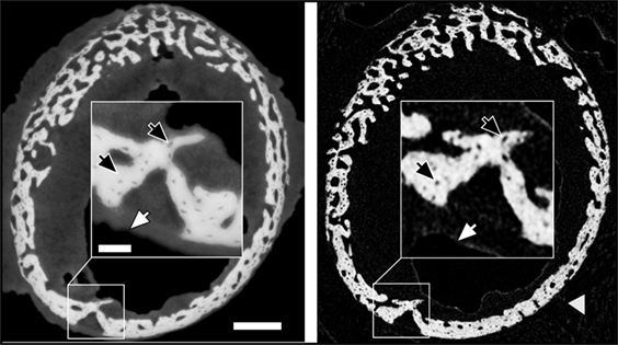
Figure 1. Comparison of similar cross-sections in a 10-day sample imaged by holotomography (left) and a laboratory source CT (right). The gray arrow head highlights gauze, which supports the bone during the lab CT scan. The scale bar equals to 200 µm. The inset shows a high magnification (scale bar = 50 µm) to highlight the differences in feature visibility between the methods. Dark arrows pinpoint osteocyte lacunae, and white arrows hint to the transition between soft tissue and air.

The reconstructed data reveals that the growing limb midshaft contains an intricate mixture of highly mineralized nodes, embedded in a 3D scaffold of structured soft tissue exhibiting substantial changes as the tissue matures. Examples of the extensive amount of detail available are shown in Figure 2 where typical cross-sections and histograms of the reconstructed density data are provided. Brighter shades of gray represent higher mass density, invariably zones of mineral density in our bone samples. The soft tissue is clearly distinguishable from both the surrounding air (black) and the higher density (bright) bone and may therefore be easily separated and identified in the 3D data. The cross-sections Figure 2A reveal extensive changes in the morphology of the bones in the first days after birth. Whereas at days 1 and 3, porous scaffolds consisting of loosely connected mineralize struts are seen, continuous growth leads toward a continuously mineralized thin outer cortex/ring of the bone midshaft appearing uniform but containing numerous cell lacunae, by 14 days. In addition to notable closing of the many pores, zones of high and low mineral density are clearly discernible. The inset figures in Figure 2B show that within the forming bone tissue, density varies considerably and that low and high mineral density zones are juxtaposed. White and dark arrows highlight example regions of differently mineralized bone that are difficult to separate in 3D by using other tomographic methods. The distributions of mass densities for entire sections of the growing femur mid diaphyses are plotted in Figure 2C. Values below a density of 0.5 g/cm³ are truncated for improved clarity. A prominent peak identified as the soft tissue peak (s) is seen with density values in the range between 1.1 and 1.4 g/cm³ in the different ages. For the very young animals a small peak presumably corresponding to cartilage (c) can also be seen. At higher densities, exceeding mass densities of ~1.6 g/cm³, a peak corresponding to bone emerges and grows with increasing age. To better interpret the information content related to both soft tissue and mineralized tissue, Figure 2D presents a magnified section of each histogram, corresponding to the soft tissue (s) and the bone (b) regions. To facilitate comparability, the data are scaled to present the soft tissue and bone peaks, respectively. A shoulder in the soft tissue peak (marked with v) appears with a slightly higher density than the main peak except in day 3, where the shoulder has a slightly lower density. The bone peaks are clearly distinguishable from the soft tissue. We identify a bone peak in the mass-density range between 1.7 and 2.0 g/cm³ with a noticeable increasing trend from 3 days on. The bone peak at day 1 is similar to the peak observed at day 14. Small shoulders in this peak are produced by islands of high mineral density within the bone (marked with *), possibly mineralized cartilage.

FIGURE 2

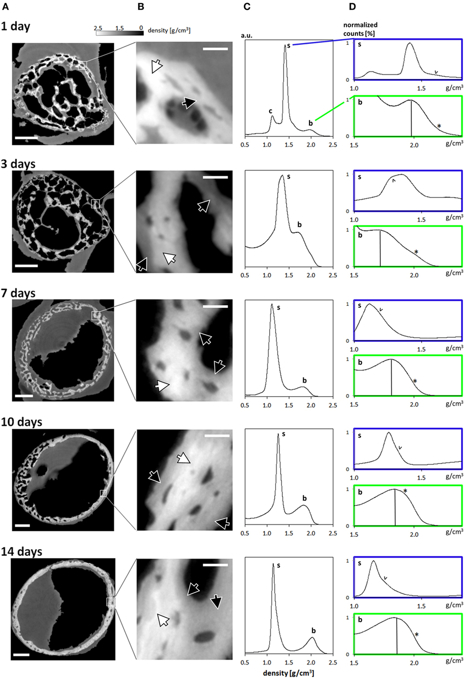
Figure 2. (A) Typical cross-sections through femur midshafts of 1, 3, 7, 10, and 14 days old mouse bones (scale bar = 200 μm). The gray values are scaled to mass density (g/cm³). (B) Insets show higher magnifications of the developing bone (scale bar = 20 μm). For clarity, the contrast is enhanced. White arrows highlight regions of highly mineralized bone, and black arrows point to low mineral regions. (C) Mass-density histograms of typical 3D datasets (more than 10⁹ values per scan) exhibiting a prominent peak of the soft tissue, a range of intermediate densities, and a shoulder depicting highly mineralized bone. (D) Magnified regions in each histogram in (B) limited to the soft tissue (s) and the bone peak (b). Within the soft tissue comprises different densities [marked by arrowheads (v)] owing to the extended holotomography density sensitivity. Vertical lines in the bone panels mark the position of the bone peak. Note the presence of substantial amounts of high mineral density bone (indicated by *).

The uniformity of the densities of both the soft tissue and bone in the different cross-sectional slices along each femur midshaft axis are demonstrated by stacked histograms plotted in Figure 3. Figure 3A demonstrates how individual histograms may be stacked to represent the soft tissue and bone density information along the bone employing a pseudo-3D representation. The color histogram highlights the counts to better visualize the peak (soft tissue and bone) heights. The position of the soft tissue peak (s) and the bone peak (b) appears to be remarkably constant along the bone axis as shown by the plots in Figure 3B. While differences can be seen between different aged bones, only minor differences can be seen at different heights along the midshaft in the distributions of soft tissue and bone within the 1-, 3-, 7-, 10-, and 14-day samples. Some minor fluctuations in the peak positions are observed in the 7-day sample.

FIGURE 3

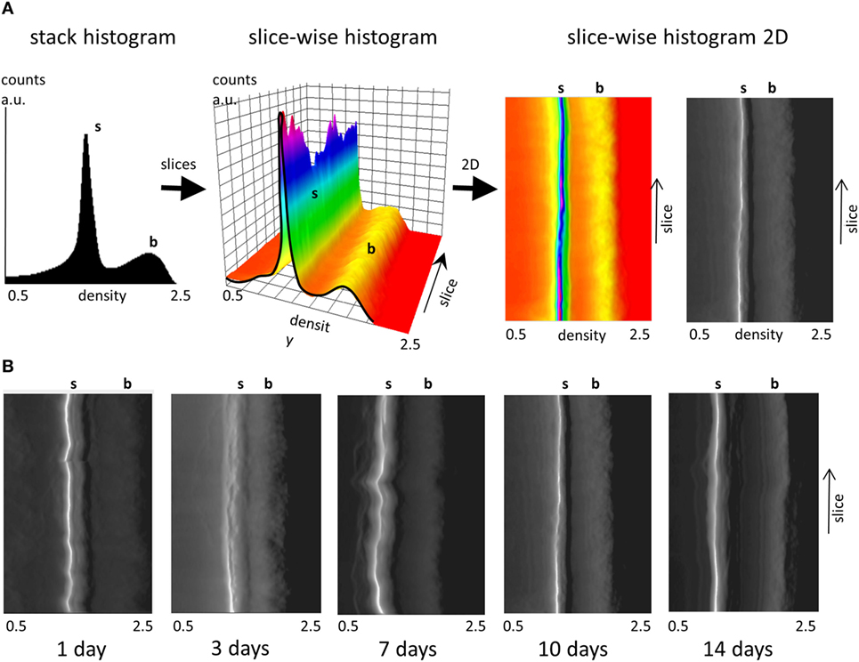
Figure 3. Slice-wise density distributions along the femur midshaft axis. (A) Transformation of a stack histogram (left) to a pseudo-3D plot of all histograms (middle) along the different slices in femur midshaft axis. The color histogram highlights the counts. When the plot is viewed from above, (right) and converted into grayscale the plot highlights the location of the soft tissue (white) and the bone peak (transition from dark gray to black). Densities between 0.5 and 2.5 g/cm³ are presented and the soft tissue and bone peak positions are highlighted (s, b). (B) Projected pseudo-3D slice-wise histograms of data stacks from 1-, 3-, 7-, 10-, and 14-day samples.

Figure 4 provides 3D renderings of the data surveyed in Figure 2, providing insight into the nature of the microstructural data in 3D. Figure 4A shows the complete gray value distribution, including the clearly distinguishable background (black) the soft tissue and the bone (different shades of gray) contributions within the reconstructed volume. The cutout in Figure 4B displayed by the dashed lines reveal the extensive details resolved within the internal structures. The exposed inner corner of the 3D cutout is magnified to provide a close-up in to the data demonstrating the available information content in the 3D datasets. The different tissues are clearly identifiable, showing the intimate spatial relationship between the bone embedded within the soft tissue. In the data obtained from a 1-day-old animal, a black arrow highlights to bone regions with greater mass density. Very thin structures are visible in the 1-day sample, marked by a gray arrowhead. Presumably, these structures transform into solid tissue during later stages of bone growth (Bortel et al., 2015). In the older samples, arrowheads highlight osteocyte lacunae that are also clearly identifiable in 3D.

FIGURE 4

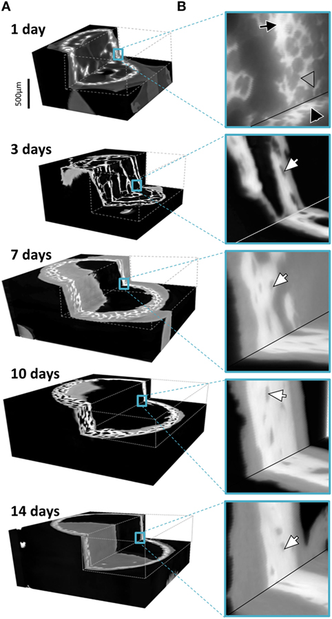
Figure 4. (A) Graphic representations of typical 3D datasets with cutouts to reveal the holotomography calculated mass-density distributions including bone and soft tissues in the developing limb structures. Note that the growing bones were scanned in air, here colorized in black, with an approximate mass density of 0, clearly distinguishable in 3D from the soft and hard tissues. (B) Insets hint to the distribution of fine details in the gray values associated with both bone and the formative soft tissues. In the 1 day data, a black arrow pinpoints bone regions with high density and very thin structures are marked by a gray arrowhead. In the older samples, arrowheads highlight osteocyte lacunae.

The different tissues can be identified based on known values of mass density. We broadly identify air, soft tissue moderately mineralized tissue and highly mineralized tissue, as displayed graphically in pseudo-3D renderings given in Figure 5. Here, blue represents the soft tissue, green is assigned to the mineralized bone, and red highlights high density islands within the bone, presumably mineralized cartilage. Similar cutouts as those used in Figure 4 reveal what the encasing soft tissue masks. For all ages, substantial amounts of soft tissue (blue) surround the forming bone material. The 3D distribution of mineralized material changes from the loosely connected foamy structures observed in the younger ages (1–7 days) into a condensed bone cortex, sandwiched between inner and outer soft tissue layers. The magnified cutouts graphically reveal the different tissues, especially the embedded high density islands (possibly mineralized cartilage) that seem to be completely encapsulated within the “normal” growing bone.

FIGURE 5

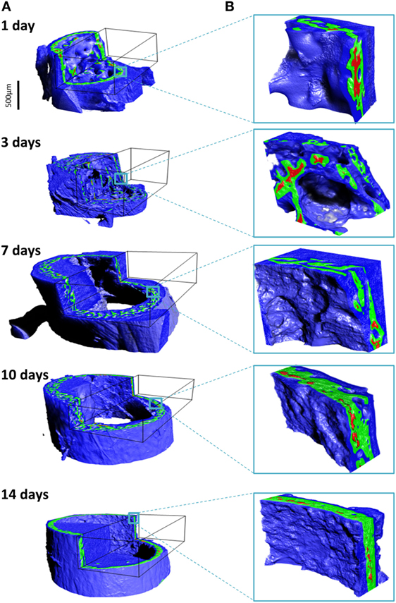
Figure 5. Density assignment and 3D mapping of the soft and hard tissues in the forming mouse femur in 3D. (A) The soft tissue colorized in blue surrounds and comes into intimate contact with mineralized bone, colorized in green. Islands of high mineral density exceeding 1.9 g/cm³ are shown in red, better observed in the high-magnification insets in (B).

Examples of separated tissues potentially ready for meshing and incorporation into finite element (FE models) are shown in Figure 6. In this representation, only the two mineral densities of bone are shown in Figure 6A. The mineralized snapshots reveal a quantitative transition from a highly porous scaffold consisting of loosely mineralized struts in the young ages into a mature solid ring seen in the samples obtained from 14 day animals. To appreciate the intricate detail, views with increasing magnification are shown in Figures 6B,C. It can be seen that the bone local morphology changes extensively with ongoing maturation, accompanied by a redistribution of high density regions located within the lower density bone. Figure 7 gives an example of a histological slice of a 14-day-old paraffin embedded mouse femur stained with Movat’s Pentachrome. Mineralized material is stained in yellow and can clearly be distinguished from the surrounding soft tissues such as the bone marrow (shades of blue) and muscle (red). In the enlarged inset, the different bone types that are present can be nicely distinguished from each other. Here, lamellar bone is located on the periosteal region (white arrows) whereas woven bone is found on the endosteal side (black arrow). Osteocyte lacunae can also be seen (gray arrowhead).

FIGURE 6

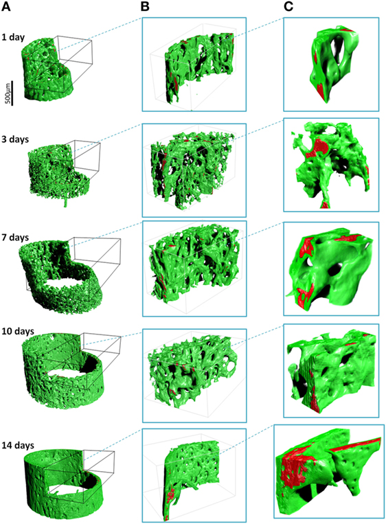
Figure 6. 3D renderings of the bone (green) and high-density zones (red) with increasing magnifications ((A), (B) and (C)). The high mass density (exceeding 1.9 g/cm³) is always found within regions of lower density. Note the drastic architectural changes from 1 to 14 days, changing from a foamy network to a solid cortical tube.

FIGURE 7

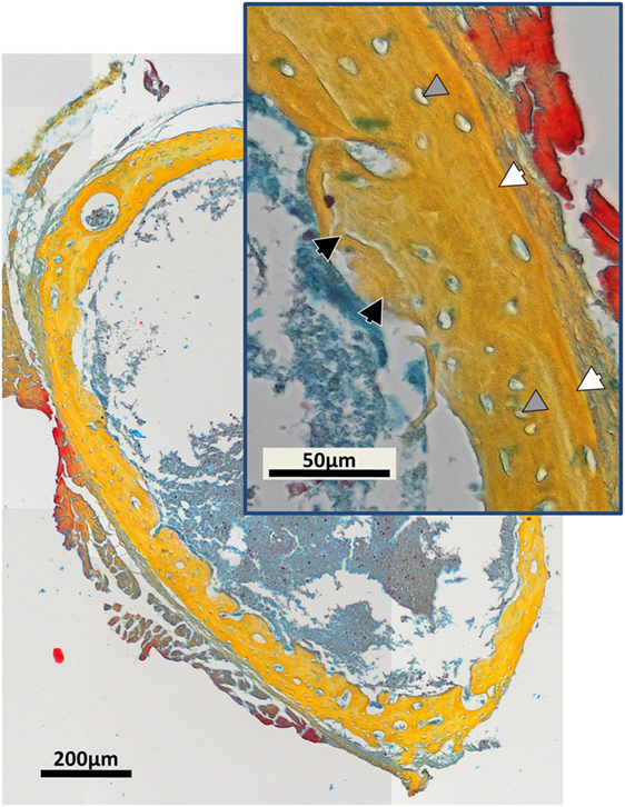
Figure 7. Movat’s Pentachrome stained typical histological cross-section of a paraffin-embedded 14-day-old mouse femur mid-diaphysis. Mineralized material is stained in yellow and can be clearly distinguished from the muscles (red) and the bone marrow (shades of blue). The inset shows a magnified region of the bone cortex. Regions of woven bone (black arrows) are seen on the endosteal surface, and lamellar bone (white arrows) is located on the periosteal region. Osteocyte lacunae can be detected (gray arrowheads).

Discussion

In this study, we demonstrate how large data in mutually aligned phase contrast-enhanced tomography datasets, processed by holotomography, reveals exquisite 3D quantitative histological-grade data in developing mouse bones. Using this approach, a large range of local gradients in density of juxtaposed soft and highly mineralized tissues are resolved down to micrometer resolution. By imaging a series of samples with increasing ages after birth we observe a host of different microstructures that are typical for the very different, normal stages of tissue formation. The complex, time-consuming sequence of acquisition and processing, currently still demanding technically, has immense potential to reveal impressive subtle structural detail in the intricate, dynamically changing forming bone tissue.

Our data reveal that in the young forming mouse bones, a mere 2–3 days are sufficient for the tissue to exhibit major transformations in the morphology of the mineralized structures. The initial formed femur bones are cylindrical scaffolds that are made of tiny discontinuous mineralized struts, clearly discernable on days 1 and 3 after birth, in 3D. These bony scaffolds increase in diameter and transform into solid mineralized tubes forming the long bone midshaft (Figures 5 and 6). The mineralized bony spicules are removed while new larger structures emerge through concerted actions of osteocytes and osteoblasts (see, e.g., Sharir et al., 2013), while the entire bone expands and enlarges. The high-resolution data shown here allows extraction of local morphological details down to the fundamental tissue ingredients including bony spicules and bone cell (osteocyte) lacunae.

In addition to the remarkable details revealed, the physical property of interest resulting from use of holotomography is a quantitative 3D distribution of mass density, which can be related to, but must be distinguished from mineral density. This paves the way to separating the complex tissue in 3D into the components of interest, as shown in Figure 5. When examining the gray value distribution of the data, the soft tissue peak exhibits density values spanning 1.1–1.4 g/cm³ for all ages. These values are slightly higher than published values for soft (skeletal) tissue (1.0–1.06 g/cm³) (itis, 2017; NIST, 2017) and cartilage (1.1 g/cm³) (itis, 2017). The higher values observed in some regions of the tissue may be due to higher concentrations of mineral precursor phases in the soft tissue, prior to bone tissue mineralization, similar to observations by other methods reported for forming bone tissue (Golub, 2009; Lange et al., 2011; Langer et al., 2012b). The bone peak becomes more prominent in histograms of bones with increasing age and reveals a high density component, presumably mineralized cartilage (Vanleene et al., 2008; Bach-Gansmo et al., 2013; Shipov et al., 2013), much of which is later replaced with more mature but less mineral-dense bone material. The data shown here make it possible to map the subtle yet important density variation in 3D, measurements that are almost impossible to perform by conventional μCT (see Figure 1).

In this work we present examples of the distribution of bone morphologies and density variations in newly formed long bones of mice. A similar approach may be used to study bone tissue growth and maturation in adult animals, during healing. Indeed, much remains unknown about the similarities and differences in the 3D bone tissue dynamics when comparing bone growth/genesis and fracture and tissue healing, e.g., in response to implantation of biomaterials. Density and the different tissue distributions in 3D presented here may help reveal the similarities and differences in bone tissue formation in these different scenarios. In recent years, a handful of studies have used holotomography and other methods in order to evaluate new biodegradable materials and treatment for healing large bone defects (Mastrogiacomo et al., 2005, 2007; Papadimitropoulos et al., 2007; Langer et al., 2010b; Ruggiu et al., 2014). Porous 3D scaffolds consisting of tricalcium phosphates (e.g., skalite) and/or hydroxyapatites seeded with different osteogenic cells were observed to promote bone formation during resorption. Newly formed bone was identified with holotomography used to quantify formed/resorbed volumes and to characterize the resulting 3D morphologies (Mastrogiacomo et al., 2005, 2007; Papadimitropoulos et al., 2007; Langer et al., 2010b; Ruggiu et al., 2014).

Growing bone in the process of mineralization contains significant non-mineralized regions. The main benefit of measuring each bone samples using five different sample-detector distances is that the quantitative density estimates provide excellent density resolution as well as impressive feature visibility. Different tissue ingredients such as soft tissue and mineralized bone morphology can clearly be separated and quantified in 3D. As seen by comparison between bones of animals with increasing ages, there is a vast amount of soft tissue that completely enwraps the mineralized compartments of the bones.

The resulting data, although challenging in terms of computational requirements, is of a size that can be further processed by available multi-processor desktop workstations, paving the way to designing computer simulations of growing and maturing bone tissues. The mechanical interactions taking place in this environment, and any mechanical stimulation leading to bone (re)modeling and structural adaptation are practically impossible to measure mechanically, and hence there is huge significance for making use of data such as presented here for producing detailed, realistic high-resolution finite element models that can faithfully reproduce and help predict changes in the micro-anatomy of the mineralizing tissue. With our detailed 3D bone/soft tissue distribution data, it becomes possible to perform virtual mechanical loading experiments, providing previously unavailable snapshots of the state of strain and stress in the tissue as it is loaded, which may be helpful for predicting the mechanical feedback related to tissue growth and adaptation. This will open up the way for future computational simulation studies of growth, healing or pathology development/treatment in bone. Such simulations might allow to separate the effects of biological signaling from the purely mechanical (strain/deformation) stimuli, which will help researchers understand the roles of physical versus chemical interactions down to the length scale of cells (e.g., by examining different “remodeling rules”; Dunlop et al., 2009; Vetter et al., 2012). This may even eventually circumvent the need to perform some of the lengthy, expensive live animal experiments, designed to study structure function relations in mechanically responsive tissues such as bone. Detailed finite element models (e.g., Varga et al., 2015) will help fill in the gaps needed to first understand and later predict tissue growth and anabolic response in the days and weeks following surgical intervention. As shown by Langer et al. (2010b), holotomography clearly resolves low-calcified pre-bone structures undergoing degradation in bone scaffold samples. Often, information on the local tissue density, readily available by holotomography, can be used as a proxy for predicting local tissue stiffness (Razi et al., 2015) important for producing realistic models of growing and forming bone tissue.

It is important to acknowledge that although within computation reach, a single final reconstructed dataset for each of the samples shown here exceeds 25 GB in size, and the intricate 3D structures that can be resolved in this data require careful processing to provide reliable 3D finite element meshes to be able to be used in realistic simulations. Bearing in mind that the final reconstruction is based on significant amounts of raw data (five scans of 4,000 images) as well as intermediate temporary files, an estimated 250 GB data and storage must be planned for each sample, which is to be considered for studies planned to include many time points or multiple measurements. Holotomography is thus yet another member of the “large data” problems requiring attention in scientific research.

As demonstrated, our holotomography data contains an abundance of spatially resolved, high-resolution data that is of high relevance for investigating growing bone morphology and structural dynamics.

Author Contributions

The experiments were planned by PF, GD, and PZ and performed by EB, JF, AR, and PZ. Data analysis and manuscript preparation were primarily done by EB, ML, and PZ. The interpretation of the data as well as manuscript development was performed by all authors equally.

Conflict of Interest Statement

The authors declare that the research was performed without any commercial or financial potential conflict of interest.

Acknowledgments

We acknowledge the European Synchrotron Radiation Facility for the provision of synchrotron radiation facility beamline ID19. We thank Prof. Dr. Stefan Mundlos for support. EB thanks the Max Planck Institute and the Berlin-Brandenburg School for Regenerative Therapies for PhD and Post-Doc funding, made possible by DFG funding through the BSRT GSC 203.

References

Bach-Gansmo, F. L., Irvine, S. C., Brüel, A., Thomsen, J. S., and Birkedal, H. (2013). Calcified cartilage islands in rat cortical bone. Calcif. Tissue Int. 92, 330. doi: 10.1007/s00223-012-9682-6

PubMed Abstract | CrossRef Full Text | Google Scholar

Bortel, E. L. (2015). Maturation of Murine Long Bones: A High Resolution Micro-Computed Tomography Study. Dissertation. Technische Universität Berlin, Berlin, Germany.

Google Scholar

Bortel, E. L., Duda, G. N., Mundlos, S., Willie, B. M., Fratzl, P., and Zaslansky, P. (2015). Long bone maturation is driven by pore closing: a quantitative tomography investigation of structural formation in young C57BL/6 mice. Acta Biomater. 22, 92–102. doi:10.1016/j.actbio.2015.03.027

PubMed Abstract | CrossRef Full Text | Google Scholar

Cloetens, P., Ludwig, W., and Baruchel, J. (1999a). Holotomography: quantitative phase tomography with micrometer resolution using hard synchrotron radiation x rays. Appl. Phys. Lett. 75, 2912. doi:10.1063/1.125225

CrossRef Full Text | Google Scholar

Cloetens, P., Ludwig, W., Baruchel, J., Guigay, J. P., Pernot-Rejmánková, P., Schlenker, M., et al. (1999b). Hard x-ray phase imaging using simple propagation of a coherent synchrotron radiation beam. J. Phys. D Appl. Phys. 32, A145. doi:10.1088/0022-3727/32/10A/330

CrossRef Full Text | Google Scholar

Dierolf, M., Menzel, A., Thibault, P., Schneider, P., Kewish, C. M., Wepf, R., et al. (2010). Ptychographic X-ray computed tomography at the nanoscale. Nature 467, 436–439. doi:10.1038/nature09419

PubMed Abstract | CrossRef Full Text | Google Scholar

Douissard, P. A., Cecilia, A., Rochet, X., Chapel, X., Martin, T., van de Kamp, T., et al. (2012). A versatile indirect detector design for hard x-ray microimaging. J Instrum 7, P09016. doi:10.1088/1748-0221/7/09/P09016

CrossRef Full Text | Google Scholar

Dunlop, J. W. C., Hartmann, M. A., Brechet, Y. J., Fratzl, P., and Weinkamer, R. (2009). New suggestion for the mechanical control of bone remodeling. Calcif. Tissue Int. 85, 45–54. doi:10.1007/s00223-009-9242-x

CrossRef Full Text | Google Scholar

Ferguson, V. L., Ayers, R. A., Bateman, T. A., and Simske, S. J. (2003). Bone development and age-related bone loss in male C57BL/6J mice. Bone 33, 387–398. doi:10.1016/S8756-3282(03)00199-6

PubMed Abstract | CrossRef Full Text | Google Scholar

Fratzl, P., Fratzl-Zelman, N., Klaushofer, K., Vogl, G., and Koller, K. (1991). Nucleation and growth of mineral crystals in bone studied by small-angle X-ray scattering. Calcif Tissue Int. 48, 407–413. doi:10.1007/BF02556454

PubMed Abstract | CrossRef Full Text | Google Scholar

Giuliani, A., Manescu, A., Langer, M., Rustichelli, F., Desiderio, V., Paino, F., et al. (2013). Three years after transplants in human mandibles, histological and in-line holotomography revealed that stem cells regenerated a compact rather than a spongy bone: biological and clinical implications. Stem Cells Transl. Med. 2, 316–324. doi:10.5966/sctm.2012-0136

PubMed Abstract | CrossRef Full Text | Google Scholar

Golub, E. E. (2009). Role of matrix vesicles in biomineralization. Biochim. Biophys. Acta 1790, 1592–1598. doi:10.1016/j.bbagen.2009.09.006

PubMed Abstract | CrossRef Full Text | Google Scholar

Guigay, J. P. (1977). Fourier transformation of Fresnel diffraction patterns and in-line holograms. Optik 46, 121–125.

Google Scholar

Hesse, B., Varga, P., Langer, M., Pacureanu, A., Schrof, S., Männicke, N., et al. (2015). Canalicular network morphology is the major determinant of the spatial distribution of mass density in human bone tissue: evidence by means of synchrotron radiation phase-contrast nano-CT. J. Bone Miner. Res. 30, 346–356. doi:10.1002/jbmr.2324

PubMed Abstract | CrossRef Full Text | Google Scholar

itis. (2017). Available at: https://www.itis.ethz.ch/virtual-population/tissue-properties/database/density/

Google Scholar

Komlev, V. S., Mastrogiacomo, M., Peyrin, F., Cancedda, R., and Rustichelli, F. (2009). X-ray synchrotron radiation pseudo-holotomography as a new imaging technique to investigate angio- and microvasculogenesis with no usage of contrast agents. Tissue Eng. Part C Methods 15, 425. doi:10.1089/ten.tec.2008.0428

PubMed Abstract | CrossRef Full Text | Google Scholar

Lange, C., Li, C., Manjubala, I., Wagermaier, W., Kuhnisch, J., Kolanczyk, M., et al. (2011). Fetal and postnatal mouse bone tissue contains more calcium than is present in hydroxyapatite. J. Struct. Biol. 176, 159–167. doi:10.1016/j.jsb.2011.08.003

PubMed Abstract | CrossRef Full Text | Google Scholar

Langer, M., Cloetens, P., Pacureanu, A., and Peyrin, F. (2012a). X-ray in-line phase tomography of multimaterial objects. Opt. Lett. 37, 2151–2153. doi:10.1364/OL.37.002151

PubMed Abstract | CrossRef Full Text | Google Scholar

Langer, M., Pacureanu, A., Suhonen, H., Grimal, Q., Cloetens, P., and Peyrin, F. (2012b). X-ray phase nanotomography resolves the 3D human bone ultrastructure. PLoS ONE 7:e35691. doi:10.1371/journal.pone.0035691

CrossRef Full Text | Google Scholar

Langer, M., Cloetens, P., and Peyrin, F. (2010a). Regularization of phase retrieval with phase-attenuation duality prior for 3D holotomography. IEEE Trans. Image Process. 19, 2428–2436. doi:10.1109/TIP.2010.2048608

CrossRef Full Text | Google Scholar

Langer, M., Liu, Y., Tortelli, F., Cloetens, P., Cancedda, R., and Peyrin, F. (2010b). Regularized phase tomography enables study of mineralized and unmineralized tissue in porous bone scaffold. J. Microsc. 238, 230–239. doi:10.1111/j.1365-2818.2009.03345.x

CrossRef Full Text | Google Scholar

Langer, M., and Peyrin, F. (2016). 3D X-ray ultra-microscopy of bone tissue. Osteoporos. Int. 27, 441–455. doi:10.1007/s00198-015-3257-0

PubMed Abstract | CrossRef Full Text | Google Scholar

Mahamid, J., Sharir, A., Gur, D., Zelzer, E., Addadi, L., and Weiner, S. (2011). Bone mineralization proceeds through intracellular calcium phosphate loaded vesicles: a cryo-electron microscopy study. J. Struct. Biol. 174, 527–535. doi:10.1016/j.jsb.2011.03.014

PubMed Abstract | CrossRef Full Text | Google Scholar

Manjubala, I., Liu, Y., Epari, D. R., Roschger, P., Schell, H., Fratzl, P., et al. (2009). Spatial and temporal variations of mechanical properties and mineral content of the external callus during bone healing. Bone 45, 185–192. doi:10.1016/j.bone.2009.04.249

PubMed Abstract | CrossRef Full Text | Google Scholar

Mastrogiacomo, M., Muraglia, A., Komlev, V., Peyrin, F., Rustichelli, F., Crovace, A., et al. (2005). Tissue engineering of bone: search for a better scaffold. Orthod. Craniofac. Res. 8, 277–284. doi:10.1111/j.1601-6343.2005.00350.x

PubMed Abstract | CrossRef Full Text | Google Scholar

Mastrogiacomo, M., Papadimitropoulos, A., Cedola, A., Peyrin, F., Giannoni, P., Pearce, S. G., et al. (2007). Engineering of bone using bone marrow stromal cells and a silicon-stabilized tricalcium phosphate bioceramic: evidence for a coupling between bone formation and scaffold resorption. Biomaterials 28, 1376–1384. doi:10.1016/j.biomaterials.2006.10.001

PubMed Abstract | CrossRef Full Text | Google Scholar

Miller, L. M., Little, W., Schirmer, A., Sheik, F., Busa, B., and Judex, S. (2007). Accretion of bone quantity and quality in the developing mouse skeleton. J. Bone Miner. Res. 2, 1037–1045. doi:10.1359/jbmr.070402

PubMed Abstract | CrossRef Full Text | Google Scholar

Mirone, A., Brun, E., Gouillart, E., Tafforeau, P., and Kieffer, J. (2014). The PyHST2 hybrid distributed code for high speed tomographic reconstruction with iterative reconstruction and a priori knowledge capabilities. Nucl. Instrum. Methods. Phys. Res. B 324, 41–48. doi:10.1016/j.nimb.2013.09.030

CrossRef Full Text | Google Scholar

Momose, A., and Fukuda, J. (1995). Phase-contrast radiographs of non-stained rat cerebellar specimen. Med. Phys. 22, 375–379. doi:10.1118/1.597472

CrossRef Full Text | Google Scholar

NIST. (2017). Available at: http://physics.nist.gov/PhysRefData/XrayMassCoef/tab2.html

Google Scholar

Nowlan, N. C., Bourdon, C., Dumas, G., Tajbakhsh, S., Prendergast, P. J., and Murphy, P. (2010). Developing bones are differentially affected by compromised skeletal muscle formation. Bone 46, 1275–1285. doi:10.1016/j.bone.2009.11.026

PubMed Abstract | CrossRef Full Text | Google Scholar

Nuzzo, S., Peyrin, F., Cloetens, P., Baruchel, J., and Boivin, G. (2002). Quantification of the degree of mineralization of bone in three dimensions using synchrotron radiation microtomography. Med. Phys. 29, 2672–2681. doi:10.1118/1.1513161

PubMed Abstract | CrossRef Full Text | Google Scholar

Paganin, D., Mayo, S. C., Gureyev, T. E., Miller, P. R., and Wilkins, S. W. (2002). Simultaneous phase and amplitude extraction from a single defocused image of a homogeneous object. J. Microsc. 206, 33–41. doi:10.1046/j.1365-2818.2002.01010.x

PubMed Abstract | CrossRef Full Text | Google Scholar

Papadimitropoulos, A., Mastrogiacomo, M., Peyrin, F., Molinari, E., Komlev, V. S., Rustichelli, F., et al. (2007). Kinetics of in vivo bone deposition by bone marrow stromal cells within a resorbable porous calcium phosphate scaffold: an X-ray computed microtomography study. Biotechnol. Bioeng. 98, 271–281. doi:10.1002/bit.21418

PubMed Abstract | CrossRef Full Text | Google Scholar

Preininger, B., Checa, S., Molnar, F. L., Fratzl, P., Duda, G. N., and Raum, K. (2011). Spatial-temporal mapping of bone structural and elastic properties in a sheep model following osteotomy. Ultrasound Med. Biol. 37, 474–483. doi:10.1016/j.ultrasmedbio.2010.12.007

CrossRef Full Text | Google Scholar

Price, C., Herman, B. C., Lufkin, T., Goldman, H. M., and Jepsen, K. J. (2005). Genetic variation in bone growth patterns defines adult mouse bone fragility. J. Bone Miner. Res. 20, 1983–1991. doi:10.1359/JBMR.050707

PubMed Abstract | CrossRef Full Text | Google Scholar

Razi, H., Birkhold, A. I., Zaslansky, P., Weinkamer, R., Duda, G. N., Willie, B. M., et al. (2015). Skeletal maturity leads to a reduction in the strain magnitudes induced within the bone: a murine tibia study. Acta Biomater. 13, 301–310. doi:10.1016/j.actbio.2014.11.021

PubMed Abstract | CrossRef Full Text | Google Scholar

Richman, C., Kutilek, S., Miyakoshi, N., Srivastava, A. K., Beamer, W. G., Donahue, L. R., et al. (2001). Postnatal and pubertal skeletal changes contribute predominantly to the differences in peak bone density between C3H/HeJ and C57BL/6J mice. J. Bone Miner. Res. 16, 386–397. doi:10.1359/jbmr.2001.16.2.386

PubMed Abstract | CrossRef Full Text | Google Scholar

Rohrbach, D., Preininger, B., Hesse, B., Gerigk, H., Perka, C., Raum, K. (2013). The early phases of bone healing can be differentiated in a rat osteotomy model by focused transverse-transmission ultrasound. Ultrasound Med Biol 39, 1642–53.

Google Scholar

Ruggiu, A., Tortelli, F., Komlev, V. S., Peyrin, F., and Cancedda, R. (2014). Extracellular matrix deposition and scaffold biodegradation in an in vitro three-dimensional model of bone by X-ray computed microtomography. J. Tissue Eng. Regen. Med. 8, 557–565. doi:10.1002/term.1559

PubMed Abstract | CrossRef Full Text | Google Scholar

Salomé, M., Peyrin, F., Cloetens, P., Odet, C., Laval-Jeantet, A.-M., Baruchel, J., et al. (1999). A synchrotron radiation microtomography system for the analysis of trabecular bone samples. Med. Phys. 26, 2194. doi:10.1118/1.598736

CrossRef Full Text | Google Scholar

Sharir, A., Milgram, J., Dubnov-Raz, G., Zelzer, E., and Shahar, R. (2013). A temporary decrease in mineral density in perinatal mouse long bones. Bone 52, 197–205. doi:10.1016/j.bone.2012.09.032

PubMed Abstract | CrossRef Full Text | Google Scholar

Sharir, A., Stern, T., Rot, C., Shahar, R., and Zelzer, E. (2011). Muscle force regulates bone shaping for optimal load-bearing capacity during embryogenesis. Development 138, 3247–3259. doi:10.1242/dev.063768

PubMed Abstract | CrossRef Full Text | Google Scholar

Shipov, A., Zaslansky, P., Riesmeier, H., Segev, G., Atkins, A., and Shahar, R. (2013). Unremodeled endochondral bone is a major architectural component of the cortical bone of the rat. J. Struct. Biol. 183, 132–140. doi:10.1016/j.jsb.2013.04.010

CrossRef Full Text | Google Scholar

Snigirev, A., Snigireva, I., Kohn, V., Kuznetsov, S., and Schelokov, I. (1995). On the possibilities of X-ray phase contrast microimaging by coherent high-energy synchrotron radiation. Rev. Sci. Instrum. 66, 5486. doi:10.1063/1.1146073

CrossRef Full Text | Google Scholar

Vanleene, M., Rey, C., and Ho Ba Tho, M. C. (2008). Relationships between density and Young’s modulus with microporosity and physico-chemical properties of Wistar rat cortical bone from growth to senescence. Med. Eng. Phys. 30, 1049–1056. doi:10.1016/j.medengphy.2007.12.010

CrossRef Full Text | Google Scholar

Varga, P., Hesse, B., Langer, M., Schrof, S., Männicke, S., Suhonen, H., et al. (2015). Synchrotron X-ray phase nano-tomography-based analysis of the lacunar-canalicular network morphology and its relation to the strains experienced by osteocytes in situ as predicted by case-specific finite element analysis. Biomech. Model. Mechanobiol. 14, 267–282. doi:10.1007/s10237-014-0601-9

CrossRef Full Text | Google Scholar

Varga, P., Pacureanu, A., Langer, M., Suhonen, H., Hesse, B., Grimal, Q., et al. (2013). Investigation of the three-dimensional orientation of mineralized collagen fibrils in human lamellar bone using synchrotron X-ray phase nano-tomography. Acta Biomater. 9, 8118–8127. doi:10.1016/j.actbio.2013.05.015

PubMed Abstract | CrossRef Full Text | Google Scholar

Vetter, A., Liu, Y., Witt, F., Manjubala, I., Sander, O., Epari, D. R., et al. (2011). The mechanical heterogeneity of the hard callus influences local tissue strains during bone healing: a finite element study based on sheep experiments. J. Biomech. 44, 517–523. doi:10.1016/j.jbiomech.2010.09.009

PubMed Abstract | CrossRef Full Text | Google Scholar

Vetter, A., Witt, F., Sander, O., Duda, G. N., and Weinkamer, R. (2012). The spatio-temporal arrangement of different tissues during bone healing as a result of simple mechanobiological rules. Biomech. Model. Mechanobiol. 11, 147–160. doi:10.1007/s10237-011-0299-x

PubMed Abstract | CrossRef Full Text | Google Scholar

Willie, B. M., Birkhold, A. I., Razi, H., Thiele, T., Aido, M., Kruck, B., et al. (2013). Diminished response to in vivo mechanical loading in trabecular and not cortical bone in adulthood of female C57Bl/6 mice coincides with a reduction in deformation to load. Bone 55, 335–346. doi:10.1016/j.bone.2013.04.023

PubMed Abstract | CrossRef Full Text | Google Scholar

Zabler, S., Cloetens, P., Guigay, J. P., and Baruchel, J. (2005). Optimization of phase contrast imaging using hard x-rays. Rev. Sci. Instrum. 76. doi:10.1063/1.1960797

CrossRef Full Text | Google Scholar

Zanette, I., Enders, B., Dierolf, M., Thibault, P., Gradl, R., Diaz, A., et al. (2015). Ptychographic X-ray nanotomography quantifies mineral distributions in human dentine. Sci. Rep. 5, 9210. doi:10.1038/srep09210

CrossRef Full Text | Google Scholar