Investigating Small-Scale Air–Sea Exchange Processes via Thermography

1. Introduction

The exchange of chemical species, including climate relevant gases such as carbon dioxide, methane and oxygen (reaeration), and of many natural and man-made volatile chemical compounds between the atmosphere and water is an important environmental process. It links the atmosphere and the hydrosphere (ocean, rivers, and lakes), has a significant influence on the global climate, and it determines the ultimate global distribution and fate of chemical trace species. On a global scale, the ocean is the largest sink for the increasing amount of atmospheric carbon dioxide (Le Quéré et al., 2014).

The exchange of gases across the air–water interface is mainly driven by the wind blowing over the sea surface. Processes taking place in the vicinity of the surface control the transport processes between the atmosphere and the oceans. On both sides of the ocean surface viscous, heat and mass boundary layers are formed, in which molecular diffusion dominates the transport. The thickness of these layers controls the speed of exchange (transfer velocity) and depends on a multitude of factors and processes that cause near-surface turbulence. In air, the mass and heat boundary layers have about the same thickness as the viscous boundary layer. In water, the mass boundary layer is much thinner (10–350 µm) than the viscous boundary layer (Figure 1), because in water molecular diffusion for mass (D) is a thousand times slower than for momentum (ν), i.e., the Schmidt number Sc = ν/D ≈ 1,000. The molecular diffusion coefficient for heat in water, D_h, is only somewhat smaller than for momentum. Therefore, the Prandtl number Pr = ν/D_h is about 7, and the thickness of the heat boundary layer lies between those of the mass and viscous boundary layer.

FIGURE 1

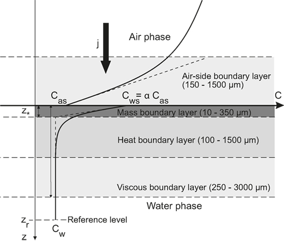
Figure 1. Sketch of the boundary layers at the air–sea interface and the mean vertical profile under steady-state conditions for a chemical species with a dimensionless solubility α (partitioning coefficient) of 3, being transported from the atmosphere into the ocean.

Exchange rates are quantified by the transfer velocity k. It is given as the ratio between the mass flux density j_c caused by the concentration difference Δc between air and water:

$k=-\frac{j_c}{c_{\text{air}}-c_{\text{water}}}=-\frac{j_c}{\Delta c},$ (1)

where the negative sign expresses the fact that the flux density is downward (negative) for positive concentration differences.

Instead of measuring the transfer velocity k directly based on the definition given above, there are two other ways, which are independent of any model assumption. Only the basic fact is used that turbulent transport is decreasing to 0 toward the water surface. Therefore, right at the water surface, the only transport mechanism is molecular diffusion. Then, the mean flux density j is directly related to the mean vertical concentration gradient via

$j=-D{{\displaystyle \frac{\partial c}{\partial z}|}}_{z=0}.$ (2)

Because of the high Schmidt number, the concentration difference is almost entirely occurring within the viscous boundary layer (Jähne, 1982). Therefore, the mass boundary layer thickness z_* is geometrically given as the interception between the tangent to the concentration profile at the water surface and the well-mixed bulk concentration c_w (Figure 1). Therefore, equation (2) can be rewritten as follows:

$j=-D\frac{c_s-c_w}{z_{\ast }}.$ (3)

Substituting equation (3) into equation (1) results in the simple relation

$k=\frac{D}{z_{\ast }}\text{\hspace{1em}or\hspace{1em}}{z}_{\ast }=\frac{D}{k}.$ (4)

In this way, the transfer velocity and the mass boundary layer thickness are inversely related to each other for a tracer with a given diffusion coefficient D. Because we know the velocity with which tracers are pushed through the mass boundary and its thickness z_*, it is easy to calculate the characteristic time constant of the transfer process across the mass boundary layer. It is given by the following equation:

$t_{\ast }=\frac{z_{\ast }}{k}=\frac{D}{k^2}.$ (5)

The relations in equations (4) and (5) mean that the transfer velocity k is directly related to the vertical length scale of the transport process, the thickness of the mass boundary layer z_*, and the time constant of the transport process t_*—without assuming any specific model about the transfer process, except that the turbulent transport term is 0 at the interface itself. Therefore, it is sufficient to measure one of these three quantities.

Excluding the high-wind speed range, gas transfer velocities for a tracer with a Schmidt number of 600 (CO₂ at 20°C; Jähne et al., 1987) range from about 2 to 70 cm/h. The corresponding mass boundary layer thicknesses z_* and time constants t_* are about 350 µm down to 10 µm and about 60 s down to 60 ms. Air–sea gas exchange is a fast process with respect to the thin mass boundary layer.

Even after 30 years of intensive research on air–water gas transfer (the 1st International Symposium on Gas Transfer at Water Surfaces took place in 1983; Brutsaert and Jirka, 1984), no satisfactory physically based model of gas transfer is available (Wanninkhof et al., 2009; Jähne, 2012; Garbe et al., 2014). Consequently, semi-empirical relationships between the gas transfer velocity k and wind speed at 10 m height, U₁₀ are still state-of-the-art. The most prominent models are Jähne (1982), Liss and Merlivat (1986), Wanninkhof (1992), and Ho et al. (2011).

A comparison of field data with some of the empirical k(U₁₀) relationships shows several interesting points (Figure 2). First, almost all measurements are performed only in a narrow wind speed range between 5 and 12 m/s. Even in this range, the measured transfer velocity may deviate from any of the relationships by more than a factor 1.7 in both directions. Second, outside of this wind speed range, there is almost no experimental data. This is not surprising for high-wind speeds larger than 12 m/s up to hurricane wind speeds of 70 m/s, because field experiments are very difficult under these conditions.

FIGURE 2

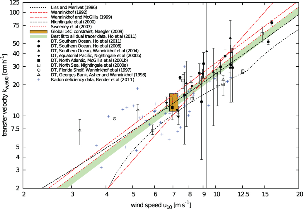
Figure 2. Gas transfer velocity as a function of the wind speed from many recent gas transfer field experiments including the dual tracer technique (DT), see Watson et al. (1991) and Wanninkhof et al. (1993), the radon deficit technique (Bender et al., 2011), and the global ¹⁴C constraint (Naegler, 2009) together with some of the empirical gas transfer velocity/wind speed relations as indicated. Drawn in logarithmic scales on both axes after Garbe et al. (2014) (Wanninkhof and McGillis, 1999; Nightingale et al., 2000; Sweeney et al., 2007).

But what about field data at low wind speeds? What is the reason for the large scatter and why are there so few data points for this regime? There are just three measurements below 4 m/s, and none below 3 m/s wind speed. This is related to the measuring technique. At 4 m/s wind speed, the transfer velocity is just about 1 m/day. Mass balance methods infer the transfer velocity from the change of concentration with time in a mass of water below the water surface, which is assumed to be well mixed. The time constant is given by the following equation:

${\tau }_{mb}=\frac{h_{eff}}{k}.$ (6)

With a mixed-layer depth of 100 m the time constant is about 100 days. Therefore, mass balance methods are not suitable at low wind speeds because wind speeds almost never remain constant for such a long time period.

A lot of hope and effort was put into the eddy covariance technique. With this method, the gas transfer velocity is measured from the covariance of the turbulent fluctuations of the vertical wind speed and trace gas concentrations averaged over a certain duration:

$k=\langle c^{\prime }{w}^{\prime }\rangle .$ (7)

The temporal resolution lies in the order of 10–60 min (Garbe et al., 2014). This is ideal for fast measurements. However, this technique only works reliably, if a sufficient concentration difference between the ocean surface waters and the atmosphere is available. Therefore—despite the much shorter measurement time compared with mass balance measurements—only about the same number of data points is available as with the mass balance method, and the scatter between the measurements is even larger (Garbe et al., 2014).

This article will focus on an alternative technique to estimate gas transfer velocities using the scalar tracer heat as a proxy for gases. It will first outline the basic principles, give an overview of the history of this technique, and explain the different measurement principles to extract transfer velocities in detail (section 2). Then, the most recent implementation of the active controlled flux technique with the new multifrequency excitation scheme, which allows for a significant increase of the temporal resolution, is presented (section 3). The article concludes with an outlook.

2. Thermographic Measurement Techniques

2.1. Basic Principle

At first glance it sounds incorrect to use heat as a proxy tracer, because heat transfer between atmosphere and ocean is controlled by the air side, while the transfer of gases with low to medium concentrations is controlled by the water side. However, the high air-side resistance for the transfer of sensible heat can be shortcut by radiative transfer, as described in more detail in section 2.3. This means that only the transfer velocity for heat from the bulk water to the water surface is measured. From this measured heat transfer velocity, the gas transfer velocity can be estimated using the dependency of the transfer velocity on the Schmidt number Sc and Prandtl number, respectively:

$k\propto D^n⇝\frac{k_{\text{gas}}}{k_{\text{heat}}}={{\displaystyle \left(\frac{\text{Sc}}{\text{Pr}}\right)}}^{-n}={{\displaystyle \left(\frac{D}{D_h}\right)}}^n.$ (8)

The exponent n is not constant. As shown experimentally by Jähne et al. (1984) and theoretically by Coantic (1986), the exponent decreases from 2/3 for a smooth water surface gradually to 1/2 for a rough and wavy water surface. The correctness of this Schmidt/Prandtl number scaling expressed in equation (8) has been verified in laboratory measurements, where heat transfer velocities and gas transfer velocities were measured simultaneously (Nagel et al., 2015).

Besides the ability to measure heat transfer rates, imaging thermography gives a direct insight into the turbulent transport processes taking place at the water surface. This has been used, for example, to study interfacial turbulence (Schnieders et al., 2013) and wave breaking (Jessup et al., 1997)

There are basically two different approaches to measure heat transfer rates via thermography: passive measurement techniques, where an existing net heat flux density at the water surface is used, and active measurement techniques, where an artificial heat flux density is applied at the water surface. The idea of passive measurement schemes is to make use of the natural effect of radiative or evaporative cooling at the water surface. Due to turbulent structures at the water surface, patterns with different temperature structures are visible and can be analyzed to estimate heat transfer velocities. The active measurements use an external heat source to obtain temperature differences at the water surface. In the following section, the historical development of both techniques will be outlined, before the sections thereafter will focus on the active controlled flux technique.

2.2. Early Measurement Techniques

The first thermographic measurements to investigate heat transfer across the aqueous air–water boundary layer were done by Jähne and Libner in the late 1980s (Libner, 1987; Libner et al., 1987; Jähne et al., 1989). Jähne introduced the controlled flux technique that is based on periodic heat excitations of the water surface and the analysis of the temperature response of the water surface.

At that time, an IR radiator was used as a heat source. This device could not be switched on and off very quickly, and thus a chopper was needed to allow for periodic heating of the water surface. Because of this mechanical device, no excitation frequencies higher than 2 Hz could be used. An IR radiometer measured the temperature response of the water surface at a small spot of cm size. About a decade later, the same principle was invented again by Wu and Busse (1998) in the field of non-destructive testing and named lock-in thermography without knowing of the earlier work in environmental science.

Another concept based on active thermography was introduced by Haußecker et al. (1995). Technological advancement had made IR cameras available, which could measure the water surface temperature accurately and with a high spatial resolution. A 25 W CO₂ laser was used to locally heat a few centimeter sized spot on the water surface. The trajectory and the temperature decay of this spot were then monitored with the IR camera. Using a surface renewal model, Haußecker derived a formula for the description of this temperature decay and was thus able to estimate heat transfer velocities.

A passive measurement approach was taken by Schimpf (Schimpf, 2000; Schimpf et al., 2004), a few years later. He observed the temperature differences at the water surface that are due to evaporative cooling. A statistical analysis of the temperature distribution at the water surface enabled Schimpf to estimate heat transfer velocities, if the heat flux could be obtained from supplementary measurements. Garbe developed an alternative approach based on passive thermography, where he could determine the heat flux directly from the analysis of flow patterns in the recorded IR images (Garbe, 2001; Garbe et al., 2003, 2004).

Haußecker’s and Garbe’s approaches rely on model assumptions for the evaluation of the data. This caused some controversies when directly measured gas transfer velocities and simultaneously measured heat transfer velocities were compared and differences between those two have been observed after Schmidt number scaling (Asher et al., 2004; Atmane et al., 2004).

As a consequence of these controversies, the original measurement scheme as proposed by Jähne et al. (1989) came up again and was reimplemented first by Popp (2006) using an IR camera instead of the IR radiometer and a 100 W CO₂ laser instead of the IR radiator and the chopper. With the IR laser it was now possible to span a wider range of excitation frequencies. This experimental setup was then used by Nagel (Nagel, 2014; Nagel et al., 2015), who could show that scaling of heat transfer velocities to simultaneously measured gas transfer velocities in a laboratory measurement reaches a good agreement. However, there still was a problem in the experimental setup used by Nagel and Popp. To heat an area on the water surface, the laser beam was expanded into a laser sheet by means of a cylindrical lens. The laser sheet was then moved forwards and backwards by a scanning mirror. However, in this way the laser’s Gaussian intensity distribution still remained along one direction of the rectangular heated area. This inhomogeneity in the heat flux density has been accounted for lately by the implementation of a new beam shaping technique based on diffractive beam homogenizers. This technique is explained in section 3.

2.3. The Controlled Flux Method

The controlled flux method inverts the principle of the commonly used mass balance methods. Instead of creating an initial concentration difference, the flux density at the water surface is controlled. The applied heat flux density causes a temperature difference between the water surface and the water beneath the heat boundary layer, which can be observed as a change in surface temperature. The basic principle is visualized in Figure 3. The controlled flux method thus requires two core components: a heat source to apply the heat flux density at the water surface and a device to monitor the temperature changes. With this instrumentation, different kinds of measurement schemes are possible, which are presented in the following sections.

FIGURE 3

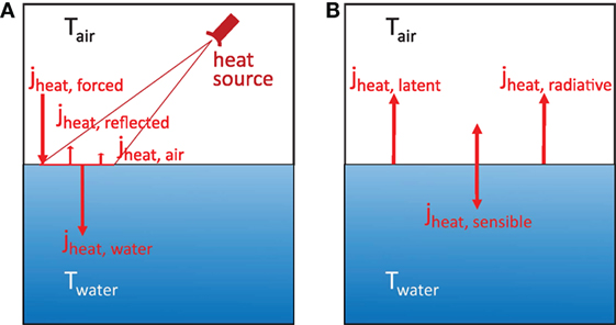
Figure 3. (A) Schematic representation of the controlled flux technique. An external heat source is used to heat the water surface and to apply a heat flux density. A small fraction of the incoming heat flux density is reflected. As the main resistance for heat transport lies on the air side, most of the heat flux will go into the water. (B) Heat fluxes at the water surface without external forcing.

2.3.1. ΔT method

In the case of heat, the transfer velocity is given by the ratio of the heat flux density j_h and the heat “concentration” difference ρc_pΔT in analogy to equation (1):

$k_h=\frac{j_h}{\rho c_{\text{p}}\Delta T}\text{\hspace{0.17em}\hspace{0.17em}or\hspace{0.17em}\hspace{0.17em}}\Delta T=\frac{j_h}{\rho c_{\text{p}}{k}_h},$ (9)

where ρ is the density of water, c_p the specific heat capacity of water at constant pressure. Since the density of water and its heat capacity are known, only the temperature difference and the heat flux density need to be measured to be able to estimate heat transfer velocities. The heat flux density can in principle be calculated from geometrical considerations:

$j_h=\frac{P_{\text{heat source}}}{A_{\text{heated}}}.$ (10)

The power of the heat source P_{heat source} is distributed across the area A_heated on the water surface by means of some beam shaping method. It can directly be seen from equation (10) that it is important to have a constant energy distribution of the heat source across the whole area that is heated. Otherwise, the heat flux density will not be constant across the whole area that is heated, and the measurement will be affected by uncertainties in the heat flux density estimation. The reason for this homogeneity constraint is illustrated in Figure 4. As a surface drift is established by the wind forcing, the water travels through the area that is heated. The water at the surface heats up with the time constant t_* given by equation (5) and thus several horizontal length scales x_* = t_* u_s are required to reach an equilibrium, where u_s is the surface drift velocity. Thus, the extension of the heated area must be large enough to enable a surface water element to reach the equilibrium temperature within the heated area. In cross-wind direction, an extension is also desired to avoid surface temperature decreases caused by horizontal turbulent diffusion.

FIGURE 4

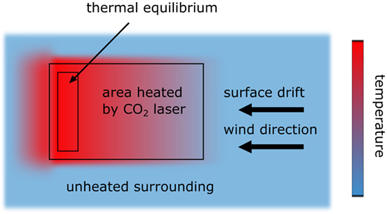
Figure 4. Heating process of the water surface seen from above. The water heats up steadily as it flows through the area that is externally heated.

As mentioned earlier, the heat flux density can be obtained via equation (10). The temperature difference needed to apply equation (9) is then simply given by the temperature difference between the equilibrium temperature region within the heated area (c.f. Figure 4) and the unheated surrounding surface water. However, at a wavy water surface, the situation becomes more difficult, and the distance between the heat source and the water surface changes with the water elevation due to the waves. Thus, equation (10) cannot directly be applied, as the size of the heated area will be affected by the changing distance between water surface and heat source as well. To overcome this problem, periodic heating of the water surface is applied. Turning the heat source on and off with a low frequency and estimating the corresponding temperature amplitude of the water surface delivers ΔT needed in equation (9). The heating frequency in this case needs to be low enough, that a water surface element can travel through the heated area until thermal equilibrium is reached within the half period of the excitation. Typically, frequencies in the order of 0.01 Hz are chosen for this purpose. In Figure 5, an example from an actual measurement used to estimate ΔT is shown. To obtain j_heat, a high frequency in the order of 25 Hz is applied. In this frequency regime, heat deposited at the water surface can only penetrate into the water for a very short distance and will thus remain at the very top of the boundary layer, where diffusion is the dominant transport mechanism. This allows to estimate the heat flux density via (Jähne et al., 1989)

$\Delta T(\omega )=\frac{j_{\text{heat}}}{\rho c_{\text{p}}\sqrt{D_h\omega }},$ (11)

with the diffusion constant of heat in water D_h. ω = 2πν is given by the excitation frequency ν used for the heat source. In this way, average values for j_heat and ΔT are obtained from the measured temperature amplitudes from two consecutive measurements with different frequencies.

FIGURE 5

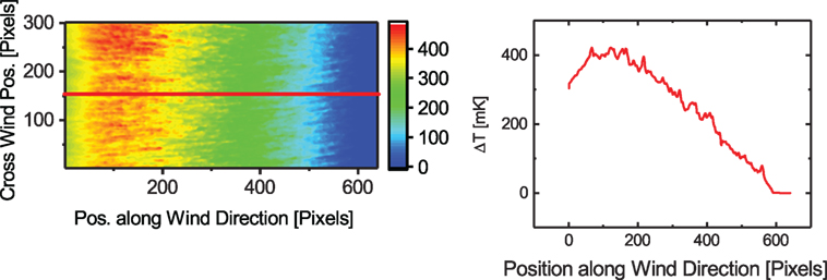
Figure 5. Actual data of a heating process as seen from above. Shown is the doubled temperature amplitude obtained for a very low excitation frequency of 0.012 Hz and for a wind speed of 1.2 m/s in the Heidelberg wind-wave facility Aeolotron. The left figure shows the heated area, and the right figure shows the temperature amplitude profile along the red line from the left figure.

2.3.2. Amplitude Damping Method

The concept based on two heating frequencies described earlier can be extended to the use of many more frequencies. This concept is the originally proposed measurement scheme from Jähne et al. (1989). This scheme is a lock-in thermographic measurement scheme, which is very robust against background signals, as for the analysis the frequency response can be filtered with respect to the known excitation frequencies. Probing the water surface with many different frequencies and analyzing the temperature response in the Fourier domain allows the study of the temporal behavior of the aqueous air–water boundary layer. Figure 6 visualizes the difference between the forcing with a low and with a high heating frequency. If the heating frequency is low, then the water surface has enough time to follow the external heating. The water will heat steadily until it reaches an equilibrium temperature and will begin to cool down, once the external heat source is switched off. In the case of a high heating frequency however, the water surface cannot follow the excitation signal. Before the temperature reaches an equilibrium upon heating, the heat source is switched off, and the water surface starts to cool down. Comparing the temperature amplitudes of the low- and high-frequency cases reveals that the temperature amplitudes of the high-frequency case are smaller and that the temperature amplitudes are thus damped. Consecutive measurements with different excitation frequencies allow to estimate the frequency, where this damping starts. Figure 7 shows an example for a measurement from the Heidelberg wind-wave facility Aeolotron, where this amplitude damping can clearly be seen. The frequency where the damping starts can be used to estimate the heat transfer velocity. At high excitation frequencies, diffusion is the dominant transport process due to the limited penetration depth of heat in water in this case. By comparing equations (2) and (11), it can be seen that two curves of the undamped and damped regime meet at the circular frequency ω_c when

${\omega }_{\text{c}}{t}_{\ast }=1.$ (12)

FIGURE 6

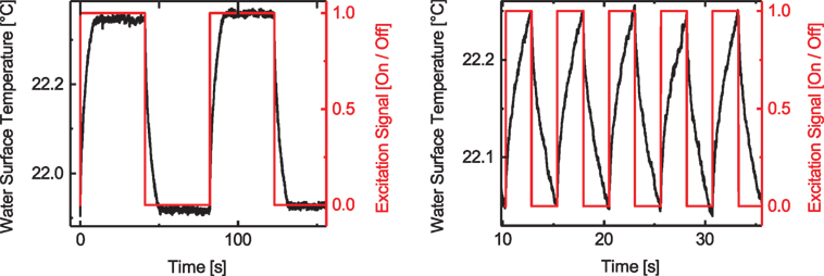
Figure 6. Temperature response of the water surface for external heating with a frequency of 0.012 Hz (left) and a frequency of 0.195 Hz (right) for a wind speed of 1.2 m/s in the Heidelberg wind-wave facility Aeolotron.

FIGURE 7

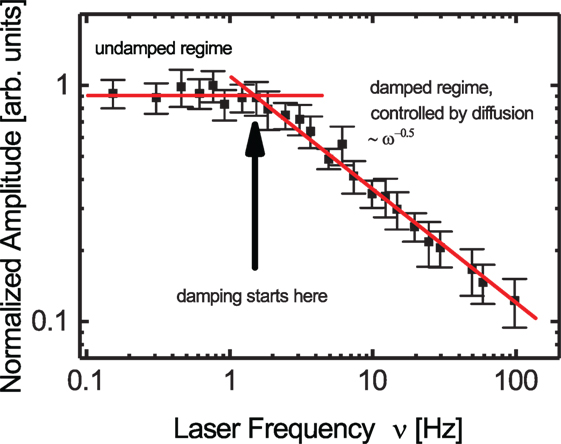
Figure 7. Normalized temperature amplitude of the water surface for different heating frequencies for a measurement with a wind speed of 3.6 m/s in the Heidelberg wind-wave facility Aeolotron. It can clearly be seen that from a certain heating frequency onward, the temperature amplitudes start to decrease.

According to equation (5), the heat transfer velocity results in

$k_{\text{heat}}=\sqrt{\frac{D}{t_{\ast }}}=\sqrt{D{\omega }_{\text{c}}}.$ (13)

This measurement scheme provides a very robust way to estimate heat transfer velocities, since the transfer velocity is obtained from several measurements with different frequencies. For the excitation signal, a square signal is chosen, as then also the third and fifth harmonic have a strong signal in the temperature spectra, and more frequencies are available for the investigation of the transfer process. An example for an excitation spectrum and the recorded temperature spectrum is shown in Figure 8.

FIGURE 8

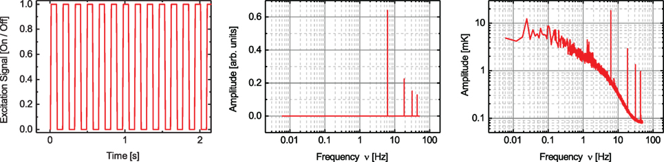
Figure 8. Example for excitation spectra of the amplitude damping method. The left figure shows the excitation signal, which is used to control the heat source. In the middle figure, the corresponding excitation spectrum is shown. The right figure shows the measured temperature spectrum of the water surface. The base frequency is 6.25 Hz. The third and fifth harmonic can clearly be seen.

3. Homogeneous Multifrequency Excitation

The amplitude damping method described earlier takes about 30–60 min for a measurement, depending on the actual boundary conditions, such as wind speed. Considering a field measurement, e.g., a measurement on board a ship on the ocean, fast measurements are demanded, as the boundary conditions cannot be controlled and might change during a measurement. The ΔT method is already much faster than the amplitude damping method, since only two frequencies are used for the excitation of the water surface. Only due to our new experiment setup, that is presented in the next section, the application of the ΔT method has become possible. The agreement of heat transfer velocities measured with the established amplitude damping method and with the ΔT method under the same conditions is very good, as shown in Figure 9. However, the two frequencies are still measured consecutively.

FIGURE 9

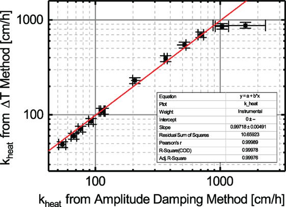
Figure 9. Comparison of heat transfer velocities obtained with the amplitude damping method and with the ΔT method for several measurement conditions in the Heidelberg Aeolotron. The agreement of both methods is excellent with a deviation of (0.3 ± 0.5%). The measurement uncertainties of the ΔT method are slightly larger than those of the amplitude damping method; however, the measurements are faster by a factor of 6–12 depending on the exact measurement condition.

To overcome this problem, a multifrequency excitation was developed (Kunz, 2017), where both frequencies are probed at the same time. Figure 10 shows exemplary excitation spectra with the overlay of a low and a high frequency. Figure 11 shows excitation signals for a 25 Hz frequency and for a multifrequency excitation with 0.049 and 25 Hz and the corresponding spectra. In Figure 12, the measured temperature amplitude spectrum for this multifrequency excitation signal is shown. The heat transfer velocity can then be estimated from such a multifrequency measurement from the measured temperature amplitudes for the low- and high-frequency according to equations (9) and (11), like for the ΔT method.

FIGURE 10

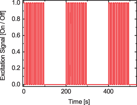
Figure 10. Example for a multifrequency excitation. A low frequency of 0.005 Hz and a higher frequency of 0.1 Hz are applied at the same time.

FIGURE 11

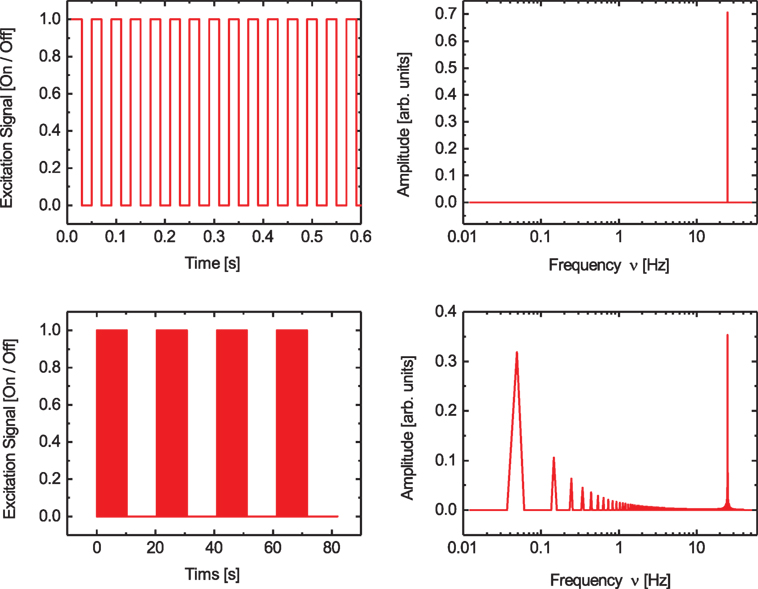
Figure 11. The upper two figures show the excitation signal and the corresponding excitation spectrum for a frequency of 25 Hz. The lower two figures show a multifrequency excitation signal with frequencies of 0.049 and 25 Hz and the corresponding excitation spectrum. The used duty cycle for both frequencies is 50%. The spectrum obtained from a measurement with this multifrequency excitation is shown in Figure 12.

FIGURE 12

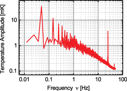
Figure 12. Measured temperature amplitude spectrum for a multifrequency excitation signal as shown in Figure 11.

A schematic drawing of the experimental setup as used in the Heidelberg wind-wave facility Aeolotron is shown in Figure 13. A carbon dioxide laser (Synrad Evolution 100, Iradion Infinity 100) operating at 10.6 µm is used as a heat source. As mentioned before, it is necessary to heat an area of around 0.25 m² homogeneously. Thus, beam shaping is required. The current setup uses a diffractive beam homogenizer (Holo/Or HH-211-A-Y-A) for this purpose. Compared with previous attempts to heat an area (c.f. Jähne et al., 1989; Popp, 2006; Nagel, 2014; Nagel et al., 2015), with such a device a significantly better homogeneity of the heat flux density can be achieved. Figure 14 shows an example of the heat signature at a calm water surface, which serves as an indicator for the beam profile at the water surface. This figure shows that the intensity distribution is not perfectly uniform. There are small speckles in the image. However, once the wind established a surface drift, and the water is pushed through the intensity pattern at the water surface, the effect of these speckles is smeared out. This is demonstrated in Figure 5, where only small ripples in the temperature profile remain as artifacts from the speckles. More important is the fact that the speckles are distributed very uniformly and randomly. Thus, it does not matter, how the exact trajectory of a water surface element looks like, when it passes through the laser profile. Figure 15 shows a comparison of the cross-wind temperature profile obtained with the old experimental setup and with the new experimental setup. It can clearly be seen that in the temperature profile from Nagel’s setup (Nagel, 2014; Nagel et al., 2015), the Gaussian intensity distribution from the laser beam is still visible. The temperature profile obtained from the diffractive beam homogenizer in contrast shows sharp edges and a distinct plateau. A comparison of heat transfer velocities measured by Nagel and by the authors with the current experimental setup using diffractive beam homogenizers is shown in Figure 16. In general, an accordance of the measurement points can be seen. However, the measurements from the new setup are much more robust, as can be seen by the relatively constant error bars. In Nagel’s data, there are several data points, where the measurement uncertainty is significantly higher compared with the newly taken data. The deviation at low friction velocities is explained by Nagel herself as the consequence of an extension of the heated area that was chosen too small in wind direction (Nagel, 2014; Nagel et al., 2015).

FIGURE 13

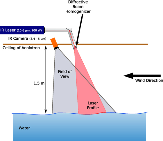
Figure 13. Schematic representation of the experimental setup as used in the Heidelberg wind-wave facility Aeolotron. An IR laser is used to heat the water surface, while an IR camera measures the temperature changes at the water surface.

FIGURE 14

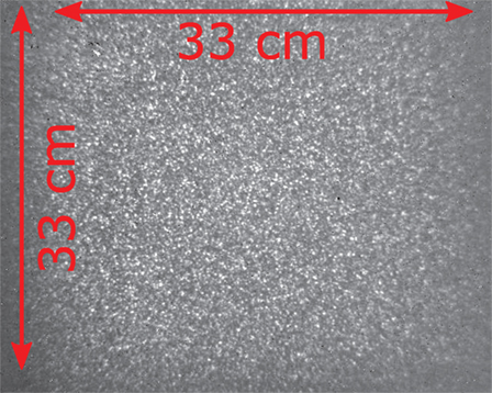
Figure 14. Example of the heat signature at the water surface for a calm condition without wind. This structure shows the intensity profile after the diffractive beam homogenizer (Holo/Or HH-211-A-Y-A). Small spots are visible; however, these structure smear out, once the water is pushed through this intensity distribution by the wind (c.f. Figure 5).

FIGURE 15

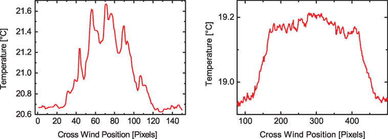
Figure 15. Comparison of cross-wind intensity distributions with Nagel’s beam shaping technique (Nagel, 2014) (left) with the current beam shaping technique based on diffractive beam homogenizers (right).

FIGURE 16

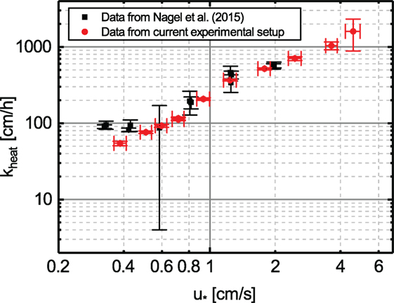
Figure 16. Comparison of data taken with the present experimental setup using a diffractive beam homogenizer and the amplitude damping method and data taken by Nagel et al. (2015) with a setup based on a cylindrical lens and a moving mirror for beam shaping and the amplitude damping method.

The temperature changes at the water surface are recorded with an IR camera (IRcam Velox 327k M) operating in the 3.4–5 µm wavelength regime with a frame rate of 100 Hz. Typical temperature amplitudes are in the order of 0.1–0.5 K. The IR camera used in our experiments has a noise equivalent temperature difference (NETD) of 20 mK and is thus a suitable detector for these small temperature changes. Camera and laser wavelengths are separated, which avoids the detection of laser reflection with the IR camera.

4. Conclusion and Outlook

As mentioned in the introduction, the main purpose of the active controlled flux technique is to measure gas transfer rates via heat as a proxy tracer with high temporal resolution. A measurement with the multifrequency scheme takes just a few min compared with hours to days as with the commonly used mass balance methods. This system also needs to be suitable for field measurements. This has been demonstrated with a previous version of the experimental setup without diffractive beam homogenizers, by Nagel (2014) during several ship based measurement campaigns.

However, there is also another major difference between mass balance techniques and the controlled flux technique for measurements in wind/wave facilities. The first one is a global measurement, averaging the measured transfer velocity over the whole water surface area of the facility. By contrast, the heat flux density is only applied locally, and only at this area the exchange process takes place. This ability to measure transfer velocities locally opens new possibilities for laboratory measurements, especially to study the dependency of the transfer velocity on fetch, the interaction length between wind and water.

To investigate to which extend the exchange rate varies with fetch, local measurements in an annular wind-wave facility, the Heidelberg Aeolotron were performed. The fetch was varied by moving a wave absorber around the annular water channel. A clear dependency of the heat transfer velocity on the fetch length can be seen for low wind speeds (Figure 17). This figure also shows the transfer velocities at infinite fetch, performed without a wave absorber. The transfer velocity increases with increasing fetch and then decreases again. This suggests that all mass balance measurements conducted in linear wind-wave facilities at low wind speeds are affected by the fetch dependence of the transfer velocity.

FIGURE 17

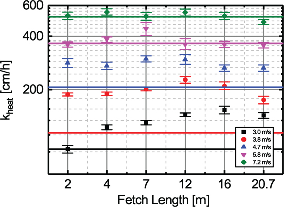
Figure 17. Heat transfer velocities measured at different fetch length in the Heidelberg wind-wave facility Aeolotron. The fetch length was varied by moving a wave absorber along the annular water channel. The solid lines represent the heat transfer velocity for infinite fetch. For low wind speeds, a clear dependency of the heat transfer velocity on the fetch length can be seen.

Measuring transfer velocities using thermography is possible in either a passive or in an active measurement scheme. The novel active controlled flux technique that has been presented can deliver transfer velocities at spatial and temporal scales unprecedented by any other field-going measurement technique available. This opens up new possibilities for field measurements. The high-temporal resolution allows for measurements under unsteady and rapidly changing conditions, and the high spatial resolution to investigate the change of the transfer velocities from clean to slick covered parts of the ocean surface.

With the newly implemented beam shaping technique based on diffractive beam homogenizers and the multifrequency excitation scheme a temporal resolution of 5 min and a spatial resolution of about 0.25 m² has been achieved.

Because imaging thermography techniques also offer a direct insight into the mechanisms of small-scale air–sea interaction processes at the air–water interface, they are very well suited for comparative studies of transport mechanisms under controlled conditions in the laboratory and under natural conditions in the field. In this way, thermographic measurements are an important means to extrapolate from laboratory to field conditions.

Author Contributions

BJ wrote the first section (Introduction) and suggested the general outline of the paper. All other sections were mainly written by JK.

Conflict of Interest Statement

The authors declare that the research was conducted in the absence of any commercial or financial relationships that could be construed as a potential conflict of interest.

Funding

Partial financial support for this work by the German Federal Ministry of Education and Research (BMBF) joint project “Surface Ocean Processes in the Anthropocene” (SOPRAN, FKZ 03F0462F, 03F0611F, and 03F0622F) within the international SOLAS project is gratefully acknowledged. The authors are grateful for financial support by the Deutsche Forschungsgemeinschaft together with the Baden-Württemberg Ministry of Science, Research and the Arts and the Ruprecht-Karls-Universität Heidelberg within the funding programme Open Access Publishing.

References

Asher, W. E., Jessup, A. T., and Atmane, M. A. (2004). Oceanic application of the active controlled flux technique for measuring air-sea transfer velocities of heat and gases. J. Geophys. Res. 109, C08S12. doi: 10.1029/2003JC001862

CrossRef Full Text | Google Scholar

Atmane, M. A., Asher, W., and Jessup, A. T. (2004). On the use of the active infrared technique to infer heat and gas transfer velocities at the air-water free surface. J. Geophys. Res. 109, C08S14. doi:10.1029/2003JC001805

CrossRef Full Text | Google Scholar

Bender, M. L., Kinter, S., Cassar, N., and Wanninkhof, R. (2011). Evaluating gas transfer velocity parameterizations using upper ocean radon distributions. J. Geophys. Res. 116, C02010. doi:10.1029/2009JC005805

CrossRef Full Text | Google Scholar

Brutsaert, W., and Jirka, G. H. (eds) (1984). Gas Transfer at Water Surfaces. Dordrecht: Reidel. doi:10.1007/978-94-017-1660-4

CrossRef Full Text | Google Scholar

Coantic, M. (1986). A model of gas transfer across air–water interfaces with capillary waves. J. Geophys. Res. 91, 3925–3943. doi:10.1029/JC091iC03p03925

CrossRef Full Text | Google Scholar

Garbe, C. S. (2001). Measuring Heat Exchange Processes at the Air–Water Interface from Thermographic Image Sequence Analysis. Dissertation, IWR, Fakultät für Physik und Astronomie, Univ. Heidelberg, Heidelberg, Germany. doi:10.11588/heidok.00001875

CrossRef Full Text | Google Scholar

Garbe, C. S., Rutgersson, A., Boutin, J., Delille, B., Fairall, C. W., Gruber, N., et al. (2014). “Transfer across the air-sea interface,” in Ocean-Atmosphere Interactions of Gases and Particles, eds P. S. Liss, and M. T. Johnson (Springer), 55–112. doi:10.1007/978-3-642-25643-1_2

CrossRef Full Text | Google Scholar

Garbe, C. S., Schimpf, U., and Jähne, B. (2004). A surface renewal model to analyze infrared image sequences of the ocean surface for the study of air-sea heat and gas exchange. J. Geophys. Res. 109, 1–18. doi:10.1029/2003JC001802

CrossRef Full Text | Google Scholar

Garbe, C. S., Spies, H., and Jähne, B. (2003). Estimation of surface flow and net heat flux from infrared image sequences. J. Math. Imag. Vis. 19, 159–174. doi:10.1023/A:1026233919766

CrossRef Full Text | Google Scholar

Haußecker, H., Reinelt, S., and Jähne, B. (1995). “Heat as a proxy tracer for gas exchange measurements in the field: principles and technical realization,” in Air–Water Gas Transfer: Selected Papers from the Third International Symposium on Air–Water Gas Transfer, eds B. Jähne, and E. C. Monahan (Hanau: AEON), 405–413. doi:10.5281/zenodo.10401

CrossRef Full Text | Google Scholar

Ho, D. T., Wanninkhof, R., Schlosser, P., Ullman, D. S., Hebert, D., and Sullivan, K. F. (2011). Toward a universal relationship between wind speed and gas exchange: gas transfer velocities measured with 3he/sf6 during the southern ocean gas exchange experiment. J. Geophys. Res. 116, C00F04. doi:10.1029/2010JC006854

CrossRef Full Text | Google Scholar

Jähne, B. (1982). “Trockene deposition von Gasen über Wasser (Gasaustausch),” in Austausch von Luftverunreinigungen an der Grenzfläche Atmosphäre/Erdoberfläche, Zwischenbericht für das Umweltbundesamt zum Teilprojekt 1: Deposition von Gasen, ed. D. Flothmann (Frankfurt: Battelle Institut), BleV–R–64. 284–2. doi:10.5281/zenodo.10278

CrossRef Full Text | Google Scholar

Jähne, B. (2012). “Gas transfer at water surfaces,” in Environmental Fluid Mechanics – Memorial Volume in Honour of Professor Gerhard H. Jirka IAHR Monograph, Chap. 22, eds W. Rodi, and M. Uhlmann (CRC Press/Balkema), 389–404.

Google Scholar

Jähne, B., Heinz, G., and Dietrich, W. (1987). Measurement of the diffusion coefficients of sparingly soluble gases in water. J. Geophys. Res. 92, 767–710. doi:10.1029/JC092iC10p10767

CrossRef Full Text | Google Scholar

Jähne, B., Huber, W., Dutzi, A., Wais, T., and Ilmberger, J. (1984). “Wind/wave-tunnel experiments on the Schmidt number and wave field dependence of air-water gas exchange,” in Gas Transfer at Water Surfaces, eds W. Brutsaert, and G. H. Jirka (Hingham, MA: Reidel), 303–309. doi:10.1007/978-94-017-1660-4_28

CrossRef Full Text | Google Scholar

Jähne, B., Libner, P., Fischer, R., Billen, T., and Plate, E. J. (1989). Investigating the transfer process across the free aqueous boundary layer by the controlled flux method. Tellus 41B, 177–195. doi:10.3402/tellusb.v41i2.15068

CrossRef Full Text | Google Scholar

Jessup, A. T., Zappa, C. J., and Yeh, H. H. (1997). Defining and quantifying microscale wave breaking with infrared imagery. J. Geophys. Res. 102, 23145–23153. doi:10.1029/97JC01449

CrossRef Full Text | Google Scholar

Kunz, J. (2017). Active Thermography as a Tool for the Estimation of Air-Water Transfer Velocities. Ph.D. thesis, Institut für Umweltphysik, Fakultät für Physik und Astronomie, Univ. Heidelberg. doi:10.11588/heidok.00022903

CrossRef Full Text | Google Scholar

Le Quéré, C., Peters, G. P., Andres, R. J., Andrew, R. M., Boden, T. A., Ciais, P., et al. (2014). Global carbon budget 2013. Earth Syst. Sci. Data 6, 235–263. doi:10.5194/essd-6-235-2014

CrossRef Full Text | Google Scholar

Libner, P. (1987). Die Konstantflußmethode: Ein neuartiges, schnelles und lokales Meßverfahren zur Untersuchung von Austauschvorgängen an der Luft-Wasser Phasengrenze. Dissertation, Institut für Umweltphysik, Fakultät für Physik und Astronomie, Univ. Heidelberg, Heidelberg, Germany.

Google Scholar

Libner, P., Jähne, B., and Plate, E. (1987). Ein neue Methode zur lokalen und momentanen Bestimmung der Wiederbeläftungsraten von Gewãssern. Wasserwirtschaft 77, 230–235. doi:10.5281/zenodo.13129

CrossRef Full Text | Google Scholar

Liss, P. S., and Merlivat, L. (1986). “Air-sea gas exchange rates: Introduction and synthesis,” in The Role of Air-Sea Exchange in Geochemical Cycling, ed. P. Buat-Menard (Boston, MA: Reidel), 113–129. doi:10.1007/978-94-009-4738-2_5

CrossRef Full Text | Google Scholar

Naegler, T. (2009). Reconciliation of excess ¹⁴C-constrained global CO₂ piston velocity estimates. Tellus B 61, 372–384. doi:10.1111/j.1600-0889.2008.00408.x

CrossRef Full Text | Google Scholar

Nagel, L. (2014). Active Thermography to Investigate Small-Scale Air-Water Transport Processes in the Laboratory and the Field. Dissertation, Institut für Umweltphysik, Fakultät für Chemie und Geowissenschaften, Univ. Heidelberg. doi:10.11588/heidok.00016831

CrossRef Full Text | Google Scholar

Nagel, L., Krall, K. E., and Jähne, B. (2015). Comparative heat and gas exchange measurements in the heidelberg aeolotron, a large annular wind-wave tank. Ocean Sci. 11, 111–120. doi:10.5194/os-11-111-2015

CrossRef Full Text | Google Scholar

Nightingale, P. D., Malin, G., Law, C. S., Watson, A. J., Liss, P. S., Liddicoat, M. I., et al. (2000). In situ evaluation of air-sea gas exchange parameterization using novel conservation and volatile tracers. Global Biogeochem. Cycles 14, 373–387. doi:10.1029/1999GB900091

CrossRef Full Text | Google Scholar

Popp, C. J. (2006). Untersuchung von Austauschprozessen an der Wasseroberfläche aus Infrarot-Bildsequenzen mittels frequenzmodulierter Wärmeeinstrahlung. Dissertation, Institut für Umweltphysik, Fakultät für Physik und Astronomie, Univ. Heidelberg. doi:10.11588/heidok.00006489

CrossRef Full Text | Google Scholar

Schimpf, U. (2000). Untersuchung des Gasaustausches und der Mikroturbulenz an der Meeresoberfläche mittels Thermographie. Dissertation, Institut für Umweltphysik, Fakultät für Physik und Astronomie, Univ. Heidelberg, Heidelberg, Germany. doi:10.11588/heidok.00000545

CrossRef Full Text | Google Scholar

Schimpf, U., Garbe, C., and JÃhne, B. (2004). Investigation of transport processes across the sea surface microlayer by infrared imagery. J. Geophys. Res. 109, C08S13. doi:10.1029/2003JC001803

CrossRef Full Text | Google Scholar

Schnieders, J., Garbe, C., Peirson, W., Smith, G., and Zappa, C. (2013). Analyzing the footprints of near surface aqueous turbulence - an image processing based approach. J. Geophys. Res. 118, 1272–1286. doi:10.1002/jgrc.20102

CrossRef Full Text | Google Scholar

Sweeney, C., Gloor, E., Jacobson, A. R., Key, R. M., McKinley, G., Sarmiento, J. L., et al. (2007). Constraining global air-sea gas exchange for CO₂ with recent bomb ¹⁴C measurements. Global Biogeochem. Cycles 21, B2015. doi:10.1029/2006GB002784

CrossRef Full Text | Google Scholar

Wanninkhof, R. (1992). Relationship between wind speed and gas exchange over the ocean. J. Geophys. Res. 97, 7373–7382. doi:10.1029/92JC00188

CrossRef Full Text | Google Scholar

Wanninkhof, R., Asher, W. E., Ho, D. T., Sweeney, C., and McGillis, W. R. (2009). Advances in quantifying air-sea gas exchange and environmental forcing. Annu. Rev. Marine Sci. 1, 213–244. doi:10.1146/annurev.marine.010908.163742

PubMed Abstract | CrossRef Full Text | Google Scholar

Wanninkhof, R., Asher, W. E., Wepperning, R., Hua, C., Schlosser, P., Langdon, C., et al. (1993). Gas transfer experiment on Georges bank using two volatile deliberate tracers. J. Geophys. Res. 98, 20237–20248. doi:10.1029/93JC01844

CrossRef Full Text | Google Scholar

Wanninkhof, R., and McGillis, W. R. (1999). A cubic relationship between gas transfer and wind speed. Geophys. Res. Lett. 26, 1889–1892. doi:10.1029/1999GL900363

CrossRef Full Text | Google Scholar

Watson, A. J., Upstill-Goddard, R. C., and Liss, P. S. (1991). Air-sea exchange in rough and stormy seas measured by a dual tracer technique. Nature 349, 145–147. doi:10.1038/349145a0

CrossRef Full Text | Google Scholar

Wu, D., and Busse, G. (1998). Lock-in thermography for nondestructive evaluation of materials. Revue Générale de Thermique 37, 693–703. doi:10.1016/S0035-3159(98)80047-0

CrossRef Full Text | Google Scholar