 Juhee Lee
 Marilou Sison-Mangus
- 1Department of Applied Mathematics and Statistics, University of California, Santa Cruz, Santa Cruz, CA, United States
- 2Department of Ocean Sciences, University of California, Santa Cruz, Santa Cruz, CA, United States
The successional dynamics of microbial communities are influenced by the synergistic interactions of physical and biological factors. In our motivating data, ocean microbiome samples were collected from the Santa Cruz Municipal Wharf, Monterey Bay at multiple time points and then 16S ribosomal RNA (rRNA) sequenced. We develop a Bayesian semiparametric regression model to investigate how microbial abundance and succession change with covarying physical and biological factors including algal bloom and domoic acid concentration level using 16S rRNA sequencing data. A generalized linear regression model is built using the Laplace prior, a sparse inducing prior, to improve estimation of covariate effects on mean abundances of microbial species represented by operational taxonomic units (OTUs). A nonparametric prior model is used to facilitate borrowing strength across OTUs, across samples and across time points. It flexibly estimates baseline mean abundances of OTUs and provides the basis for improved quantification of covariate effects. The proposed method does not require prior normalization of OTU counts to adjust differences in sample total counts. Instead, the normalization and estimation of covariate effects on OTU abundance are simultaneously carried out for joint analysis of all OTUs. Using simulation studies and a real data analysis, we demonstrate improved inference compared to an existing method.
1. Introduction
Microbial communities are influenced by several factors whether they live in the host's guts or other occupied niches. Their successional dynamics could further change in response to perturbations of the host or of the surrounding environments (Turnbaugh et al., 2009; Needham and Fuhrman, 2016). Understanding how abiotic and biotic factors influence the dynamics of microbial communities is of great interest in the field of microbiome studies. Recent revolutionary advances in next-generation sequencing (NGS) technologies along with rapidly decreasing costs, have facilitated the accumulation of large datasets of 16S ribosomal RNA (rRNA) amplicon sequences across various disciplines such as medicine, biology, ecology, and environmental sciences (Woo et al., 2008). Sequencing data is usually pre-treated for quality filtering, noise removal and chimera checking through bioinformatics algorithms and the filtered sequences are clustered into Operational Taxonomic Units (OTUs), which represent similar organisms (microbial species) based on sequence homology (called OTU picking). An OTU abundance table is generated, recording counts for OTUs in samples. Further statistical data analyses are then performed using the OTU table to answer biological and ecological questions.
Analysis of huge NGS data is computationally expensive and challenging. One of the key challenges is the normalization of counts across samples. Total counts (often called library size or sequencing depth) may vastly vary across different samples due to technical reasons. Thus, observed counts are not directly comparable across samples and cannot be used as a measure of the abundance of an OTU. Normalized counts through rarefaction or relative frequencies are commonly used for easy comparison of OTU abundance across samples. However, such ad hoc normalization procedures have been criticized from a statistical perspective since using pre-normalized quantities may undermine the performance of downstream analysis (McMurdie and Holmes, 2014). Another challenge is high dimensionality and sparsity in OTU count data. A dataset typically includes hundreds or thousands of OTUs and a majority of them has zero or very low frequencies in most of samples. For example, Figure 1A illustrates a heatmap of OTU counts in our motivating dataset described in section 2.3. It shows that a majority of OTUs has very low counts (gray) in a sample, and the set of OTUs having large counts (blue) vary across samples. Due to such sparsity in data, borrowing strength across OTUs through joint analysis of all OTUs is crucial for improved inference. Recently, various statistical methods including Romero et al. (2014), Chen and Li (2016), Gibbons et al. (2017), and Zhang et al. (2017) have been developed for microbiome studies using NGS data. For example, Zhang et al. (2017) used a negative binomial mixed regression model to study interactions between the microbiome and host environmental/clinical factors. Random effects are used to induce correlation among samples from a group. Common to most of recent methods including Zhang et al. (2017) is separately analyzing each OTU at a time.
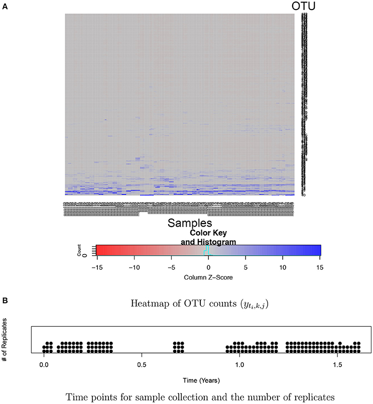
Figure 1. Ocean microbiome data. (A) Heatmap of OTU counts (yti,k, j). OTU and samples are in rows and columns, respectively. OTU counts are rescaled within a sample for better illustration. (B) 55 time points where ocean microbiome samples were collected are marked on the X-axis and the number of dots at a time point represents the number of replicates (Ki) at the time point.
We develop a Bayesian semiparametric generalized linear regression model to study the effects of physical and biological factors on abundance of microbes. The proposed method performs mode-based normalization through a hierarchical model, which enables direct modeling of OTU counts. Furthermore, the hierarchical model facilitates borrowing strength between OTUs, between samples, and between time points through joint analysis and improves inference on the effects of covariates X on OTU abundance which are the parameters of our primary interest. Specifically, a negative binomial (NB) distribution parameterized by a mean parameter μ and an overdispersion parameter s is assumed for OTU counts. The NB distribution flexibly accommodates overdispersion often seen in NGS data and is commonly used as a robust alternative to a Poisson distribution (Anders and Huber, 2010). The expected count μ of an OTU is decomposed as a product of factors, a baseline mean count g and a nonnegative function η(X) of covariates that describes their effects on the mean count. We use the log link function for η(X) and assume that change in a covariate has a multiplicative effect on mean count, where the associated coefficient quantifies the size and direction of the effect. We consider a Laplace prior for the coefficients, a shrinkage prior that is essential in a high dimensional regression setting. Shrinkage priors in regression yield sparse point estimates of the coefficients, where many of the coefficients have values close to zero and few have large values. The sparse estimates improve out-of-sample prediction and produce more interpretable models (Park and Casella, 2008). In addition, shrinkage priors such as a Laplace prior in a regression problem mitigate potential problems by multicollinearity and yield improved coefficient estimates when covariates are high-dimensional and potentially highly correlated (Polson and Scott, 2012). For baseline mean counts, we develop a nonparametric model to combine all OTUs for joint analysis. Baseline mean counts may vary across samples and OTUs. Also, as in our motivating data for which samples were taken over time, there may be temporal dependence in baseline mean counts. To tackle the problem, we further decompose the baseline count g into sample size factor (r), OTU size factor (α0), and OTU and time factor (αt), that is, g = r × α0 × αt. Due to the overparametrization of the baseline mean abundance, individual factors are not identifiable. To avoid identifiability issues, we place the regularizing priors with mean constraints (Li et al., 2017) for sample size factor r and OTU size factor α0. In addition, we model a temporal dependence structure between the baseline expected counts for an OTU through a convolutional Gaussian process (Higdon, 1998). The process convolution approach is often used as an alternative approach of the Gaussian process to construct a dependent process due to its efficient computation (Lee et al., 2005; Liang and Lee, 2014). Through simulation studies, we show that estimates of individual parameters r, α0, and αt are not fully interpretable under the proposed model, but baseline mean counts g are identifiable. The model also provides a posterior distribution of g for uncertainty quantification.
The rest of the paper is organized as follows. In section 2 we describe the proposed model and discuss the prior formulations and the resulting posterior inference. We perform simulation studies to assess the proposed model and perform comparison with an existing method that analyzes one OTU at a time. We then apply the proposed model to an ocean microbiome dataset. Section 3 presents the performance of the proposed model from the simulation experiment and the ocean microbime data. Section 4 concludes the paper with a discussion on limitations and possible extensions.
2. Materials and Methods
2.1. Bayesian Semiparametric Regression Model
Suppose that samples are taken at n different time points, 0 ≤ ti ≤ T, i = 1, …, n, and with Ki replicates at time point ti. We consider count yti,k, j of OTU j in replicate k taken at time ti, where i = 1, …, n, k = 1, …, Ki, and j = 1, …, J. A sample is thus indexed by ti and k. We let the total number of samples . Let Y = [yti,k, j] denote the N×J matrix of counts, where yti,k, j is integer-valued and nonnegative. Also, suppose that covariates are recorded at time ti. For example, covariates are physical and biological factors in our motivating data.
2.1.1. Sampling Model
Count data by NGS methods is often modeled through a Poisson distribution. The assumption under the Poisson distribution that the variance is equal to the mean is often too restrictive to accommodate overdispersion that variation in data exceeds the mean. The negative binomial (NB) distribution is a popular and convenient alternative to address the overdispersion problem and is widely recognized as a model that provides improved inference to NGS count data (for example, see Robinson and Smyth, 2007; Anders and Huber, 2010). A NB distribution can be characterized by mean and overdispersion parameters. We suppress index i for simpler notation and assume a NB model for count yt,k,j of OTU j in replicate k at time t,
where mean count μt,k,j > 0 and overdispersion parameter sj > 0. The model in Equation (1) implies that count of OTU j in replicate k at time t has mean E(yt,k,j ∣ μt,k,j) = μt,k,j and variance . The model allows different dispersion levels across OTUs through OTU-specific overdispersion parameters sj. In the limit as sj → 0, the model in Equation (1) yields the Poisson distribution with mean μt,k,j. We assume a gamma distribution for a prior distribution of sj, , j = 1, …, J, with fixed as and bs.
2.1.2. Model for Regression
We next model the mean count μt,k,j of yt,k,j. We decompose the mean count into factors, a baseline mean count and a function of covariates, μt,k,j = gt,k,jηj(Xt). Here parameter gt,k,j denotes the baseline mean abundance of OTU j in sample (t, k) and ηj(Xt) is a function of covariates Xt for OTU j to model the covariate effects. We construct a generalized regression model by letting , where is a P-dimensional vector of regression coefficients of OTU j (Lawless, 1987; McCullagh and Nelder, 1989). The coefficient βj, p quantifies the effect of covariate p Xp on the mean abundance of OTU j. A vector βj close to the zero vector produces a value of ηj(Xt) close to 1, and the mean count remains similar to the baseline mean count gt,k,j, implying insignificant covariate effects. A negative (positive) of βj, p implies a negative (positive) association between mean counts and the p-th covariate, and a larger value of Xj,p decreases (increases) the mean count, while holding the other covariates constant. We consider a Laplace prior on βj. Specifically, we express the Laplace distribution as a scale mixture of normals and assume for j = 1, …, J and p = 1, …, P,
where aλ, bλ, aσ, and bσ are fixed. and ϕj,p denote the global and local shrinkage parameters, respectively, for OTU j. After integrating ϕj,p out, the prior distribution of βj,p is the Laplace distribution with location parameter 0 and scale parameter , that is, . Compared to a normal distribution that is a common choice for the prior of βj,p, the Laplace distribution has more concentration around zero but allows heavier tails. The regularized regression through the Laplace prior more shrinks the coefficients of insignificantly related covariates into zero and less pulls the coefficients of important covariates toward zero. Shrinkage of β estimates through the model in Equation (2) mitigates possible issues due to multicollinearity and efficiently improves estimation of β in a high dimensional setting (Polson and Scott, 2012).
2.1.3. Model for Baseline Mean Count
We next build a prior probability model for the baseline mean count gt,k,j of OTU j in sample (t, k). We assume gt,k,j = rt,kα0, jαt, j to separate sample (rt,k), OTU (α0, j), and OTU-time (αt, j) factors. Sample total counts may greatly differ for different samples possibly due to experimental artifacts. For example, counts of an OTU even in the replicates taken at a time point may vastly differ. Sample specific size factors rt,k account for different total counts in different samples and expected counts normalized by rt,k are comparable across samples. Factor α0, j explains variabilities in baseline mean abundances of OTUs and αt,j models temporal dependence of the mean counts for an OTU, respectively. Factors α0, j and αt,j are not indexed by replicate k and account for stochastic change over time in normalized baseline expected counts of OTU j. Collecting all, we write the mean count as
The model for gt,k,j in Equation (3) is overparameterized and the individual parameters are not identifiable. To avoid potential identifiability issues, many of NB models rely on some form of approximation for the baseline mean counts. For example, one may find the maximum likelihood estimates (MLEs) of baseline mean abundance under some constraints and plug in those estimates to infer the mean abundance levels μti, j of OTUs (Witten, 2011). Plugging in MLEs is simple but may not be robust. In particular, the inference is greatly affected by a small change in a few OTUs that have large counts. Moreover, the errors introduced in the baseline mean count estimation will not be reflected in the inference. Several approaches to robustify the estimates are proposed (for example, see Anders and Huber, 2010; Witten, 2011). To circumvent the identifiability issue and provide uncertainty quantification for estimation of gt,k,j, we take an alternative in Li et al. (2017) by imposing regularizing priors with mean constraints for rt,k and α0, j. We let the logarithm of the factors and , and assume the regularizing prior distribution with mean constraints,
where ϕ(η, v2) is the probability density function of the normal distribution with mean η and variance v2, constraints for the mixture weights with and , , and for all ℓ. Mixture models as in Equation (4) are often used as a basis to approximate any distribution. Each component in Equation (4) is further composed of a mixture of two normals, and with weights wℓ and 1 − wℓ, respectively, and the mean of the component is c. In consequence, the prior and posterior of and under the model in Equation (4) satisfy their prespecified mean constraints cr and cα, respectively. Li et al. (2017) showed that the model in Equation (4) flexibly accommodates various features in a distribution such as skeweness or multi-modality while satisfying the constraints. Furthermore, the model based normalization through Equation (4) enables joint analysis of all OTUs and can further improve estimation of the covariate effects. With the regularizing priors, baseline mean counts gt,k,j are identifiable, while rt,k, α0, j, and αt,j are not directly interpretable. More importantly, the parameters of primary interest ηj(Xt) can be uniquely estimated and βj,p's keep their interpretation as parameters that quantify the effects of covariates on mean counts. We used an empirical approach to fix the mean constraints cr and cα. Sensitivity analyses were conducted to assess the robustness to the specification of cr and cα and show that the model provides reasonable estimates of gt,k,j and moderate changes in the values of cr and cα minimally change the estimates. More details of the specification of cr and cα are discussed in section 3.1. We fix the numbers of mixture components, Lr and Lα and variances and . We let and , where and are fixed. We assume and , with fixed dr and dα. We let , ℓ = 1, …, Lr and , ℓ = 1, …, Lα with fixed ar, br, aα, and bα.
Recall that samples are collected over time points t1, …, tn in [0, T] and αt,j accounts for temporal dependence in the baseline mean count for an OTU. We let a function in time t and use a stochastic process to model temporal dependence among μt,k,j. The Gaussian process (GP) is one of the most popular stochastic models for the underlying process in spatial and spatio-temporal data (for example, see Cressie, 1992; Banerjee et al., 2014 among many others). The GP effectively represents the underlying phenomenon in a variety of applications, but it has some drawbacks such as a complex computation that requires a matrix decomposition and problematic estimation of the parameters in its covariance function, potentially leading to difficulties in exploring the posterior distribution (Lee et al., 2005; Liang and Lee, 2014). To alleviate such difficulties of GP models while still maintaining their flexibility and adaptiveness, we use a convolution approach with a kernel function developed in Higdon (1998, 2002). For each OTU, we specify the latent process θj(t) to be nonzero only at the time points u1, …, uM in [0, T]. Specifically, we consider the GP convolution model,
where {u1, …, uM} a set of basis points in with , and Z(t − um) a Gaussian kernel centered at um, . The number of basis points M, their locations um and the range parameter γ can be treated as random variables by placing prior distributions, e.g., consider a gamma prior for γ. For simplicity, we fix them as follows. We first choose a value for M and let um evenly spaced over time . Following Xiao (2015), we let the range parameter , that is, the range parameter depends on the value of M. Through simulations, we studied the impact of different values of M on the posterior inference of gt,k,j. A discussion is included in section 3.1. Given the number of basis points M, we assume and , m = 1, …, M and j = 1, …, J.
We implement posterior inference on the parameters via a Markov chain Monte Carlo (MCMC) method based on Metropolis-Hastings algorithm and Gibbs sampling. Each of the parameters is iteratively updated conditional on the currently computed values of all other parameters to simulate a sample from the posterior distribution. The parameters and jointly determine baseline mean counts and joint updating of and may greatly improve the mixing. In our ocean microbiome data, some discretized covariates are missing. We treat them as random variables by assuming a uniform distribution over possible categories, and impute their values in MCMC simulation. Full details of our MCMC algorithm are given in Supplementary section 1. We diagnose convergence and mixing of the described posterior MCMC simulation using trace plots and autocorrelation plots of imputed parameters. For the upcoming simulation examples and the data analysis, we found no evidence of practical convergence problems. An R package of the code used for simulations and the analysis of the ocean microbiome dataset in the following sections is available from the authors website https://users.soe.ucsc.edu/~juheelee/.
2.2. Simulation Experiment: Data Generation and Comparative Study
We conducted simulation studies to assess the performance of our model. We compared the model to an alternative model, the negative binomial mixed model (NBMM) in Zhang et al. (2017). We assumed a sample of J = 200 OTUs. We used the same time points (ti) and numbers of replicates (Ki) of our ocean microbiome data as shown in Figure 1B. We let with probability 0.85. For we simulated from either of N(−1.5, 0.052) or N(1.5, 0.052) with equal probability, where N(a, b2) denotes the normal distribution with mean a and variance b2. It implies that a covariate has no effect on OTU abundance with probability 0.85 or may significantly affect mean abundance with the remaining probability 0.15. To specify and , we did not assume any distribution and used their classical estimates from our ocean microbiome data; following Witten (2011), we first computed estimates of sample size factors and OTU size factors using the ocean microbiome data, and where and . We then randomly sampled from the pool of and to specify the true values. To simulate temporal dependence in OTU abundance, we let Here denotes time ti in year and the median of . We let , , and to have different patterns for OTUs. For some OTUs, are illustrated in red squares in Figures 4E–G. We generated . We used the covariate matrix of the ocean microbiome data illustrated in Figure 2 for the simulation study. For the missing covariates in the data, we generated a value of possible categories with equal probability. We finally simulated OTU counts yti,k, j from the negative binomial distribution where .
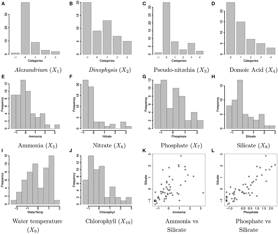
Figure 2. Ocean microbiome data. Bar plots of discretized covariates, concentration levels of Alexandrium (Ax, X1) and Dinophysis (Dp, X2), Pseudo-nitzchia (Pn, X3), domoic acid (DA, X4) in (A–D). The values of −1, 0, 1, 2, 3, and 4 represent a missing value, none and low, medium, high, and highest concentration levels, respectively. Histograms of continuous covariates, concentration levels of ammonia (NH4, X5), nitrate (N, X6), phosphate (P, X7), silicate (Si, X8), water temperature (T, X9), concentration level of chlorophyll (Chl, X10) in (E–J). The variables are standardized to have mean 0 and variance 1 prior to analysis. A scatterplot of the concentrations of ammonia and silicate and a scatterplot of the concentrations of phosphate and silicate are shown in (K,L), respectively.
For comparison, we used the negative binomial mixed model (NBMM) in Zhang et al. (2017). Similar to the proposed model, the NBMM uses a negative binomial distribution with mean μNBMM and shape parameter θNBMM to model OTU counts and assumes where Xt and Zt,k are the covariate matrices for fixed effects and random effects, respectively. It assumes random effects . By letting the replicates at a time point share the same random effect, OTU abundances in the replicates at a time point are correlated. The NBMM normalizes OTU counts by sample total counts. That is, sample total counts yt,k, · are used as an offset to adjust for the variability in total counts across samples. Similar to other existing methods, the NBMM performs separate analyses of OTUs. An iterative weighted least squares algorithm is developed to produce the MLEs under the NBMM and implemented in a R function glmm in R package BhGLM.
2.3. Ocean Microbiome Data: Data Description and Preprocessing
We applied the proposed statistical method to ocean microbiome data. Seawater samples were collected weekly at the end of Santa Cruz Municipal Wharf (SCW), Monterey Bay (36.958 oN, −122.017 oW), with an approximate depth of 10 m. SCW is one of the ocean observing sites in Central and Northern California (CenCOOS), where harmful algal bloom species [HAB species: Alexandrium (Ax), Dinophysis (Dp), Pseudo-nitzschia (Pn) etc.] are monitored weekly along with nutrient measurements [ammonia (NH4), silicate (Si), nitrate (N), phosphate (P)], temperature (T), domoic acid (DA) concentration, and chlorophyll (Chl). Details of phytoplankton net tow sampling of measuring phytoplankton abundance, measurement of physical (nutrients and temperature) and biological parameters (chlorophyll α and DA concentration) are described in Sison-Mangus et al. (2016). Pseudo-nitzschia, Dinophysis, and Alexandrium cells were counted with a Sedgewick rafter counter under the microscope. Data for physical and biological factors are available from the website link http://www.sccoos.org/query/?project=Harmful%20Algal%20Blooms&study[]=Santa%20Cruz%20Wharf. Among the 10 variables, the concentration levels of Alexandrium, Dinophysis, Pseudo-nitzschia, and domoic acid have highly right-skewed distributions and are discretized into categories based on their biological properties for our analysis. The ranges of the concentration levels for the discretization are in Supplementary Table 1 and Figures 2A–J illustrates all covariates included for analysis. The values of −1, 0, 1, 2, 3, and 4 represent missing values and the categories of None, Low, Medium, High, and Very High for the discretized variables, respectively. Due to high right skeweness, categories corresponding to high concentration levels have low frequencies. Values of the Dinophysis concentration level are missing at 20 time points among 55 points used for analysis. Sample correlations between the factors are relatively strong. Figures 2K,L shows scatterplots for some selected pairs of the factors.
For bacterial RNA samples, three depth-integrated (0, 5, and 10 ft) water samples were collected at a total of 55 time points between April 2014 and November 2015. Two or three samples are sequenced at each time point. The numbers of replicates at the time points are illustrated in Figure 1B. Microbial RNA in the samples was extracted for 16S rRNA sequencing. Post-processing of sequences was performed using the Quantitative Insights Into Microbial Ecology (QIIME 1.9.1) pipeline. A total of nearly 39,823 OTUs were obtained in data after removing singletons. We restricted our attention to OTUs that have greater than or equal to five counts on average. The rule leaves in the end J = 263 OTUs for the 150 samples for the analysis. A heatmap of the counts in the filtered data is shown in Figure 1. The primary goal of the study is to investigate the effects of physical and biological factors on abundance levels of OTUs, while accounting for baseline abundance levels of OTUs in samples.
3. Results
3.1. Simulation Experiment: Model Fitting and Comparison
To fit the proposed model for the simulated data designed in section 2.2, we specified hyperparameter values of the model as follows; for the Laplace prior of βj,p, we let aλ = bλ = 0.5 for a gamma prior of (with mean aλ/bλ and variance ) and aσ = bσ = 0.3 for an inverse gamma prior for common variances . For the regularizing priors of and , we fixed dα = dr = 10, ar = br = aα = bα = 1, , , and . We also fixed the number of mixture components for the regularizing priors Lr = 30 and Lα = 50. To specify values of the mean constraints cr and cα, we took an empirical approach. We used the simulated yti,k, j, computed estimates of rti,k, j and αj, 0 as described in section 2.2 and fixed the mean constraints at the means of the logarithm of the estimates, respectively. Note that the specified values of cr and cα were very different from the means of their true values. For the process convolution prior of OTU-time factor , we chose a value of M such that the kernel function at a basis point is not entirely located in a place where no sample is obtained. We let the number of basis M = 13 and basis um, m = 1, …, M evenly spaced between −10 and Ti + 10. For overdispersion parameter sj we let as = 1 and bs = 2. To run MCMC simulation, we initialized the parameters by simulating with their prior distributions. We then implemented posterior inference using MCMC simulation over 25,000 iterations, discarding the first 10,000 iterations as burn-in and choosing every other sample as thinning.
Figure 3 illustrates the comparison of posterior estimates of βj,p to their true values for some selected covariates. In the figure, dots and blue dashed lines represent posterior means of βj,p and their 95% credible intervals, respectively. s are around the 45 degree line (red dotted line) for most of (j,p) and most of the interval estimates captures the true values. It implies that the proposed model reasonably recovers . For categories 3 and 4 of X4 in Figures 3I,J, the credible intervals tend to be wider due to their low frequencies in the data as shown in Figure 2D. The insert plot in each panel illustrates a scatter plot of for (j,p) with . It shows that the proposed regression model with the Laplace prior effectively shrinks βj,p with to zero, as is desired in our simulation setup. Supplementary Figure 1 has plots for all covariates.
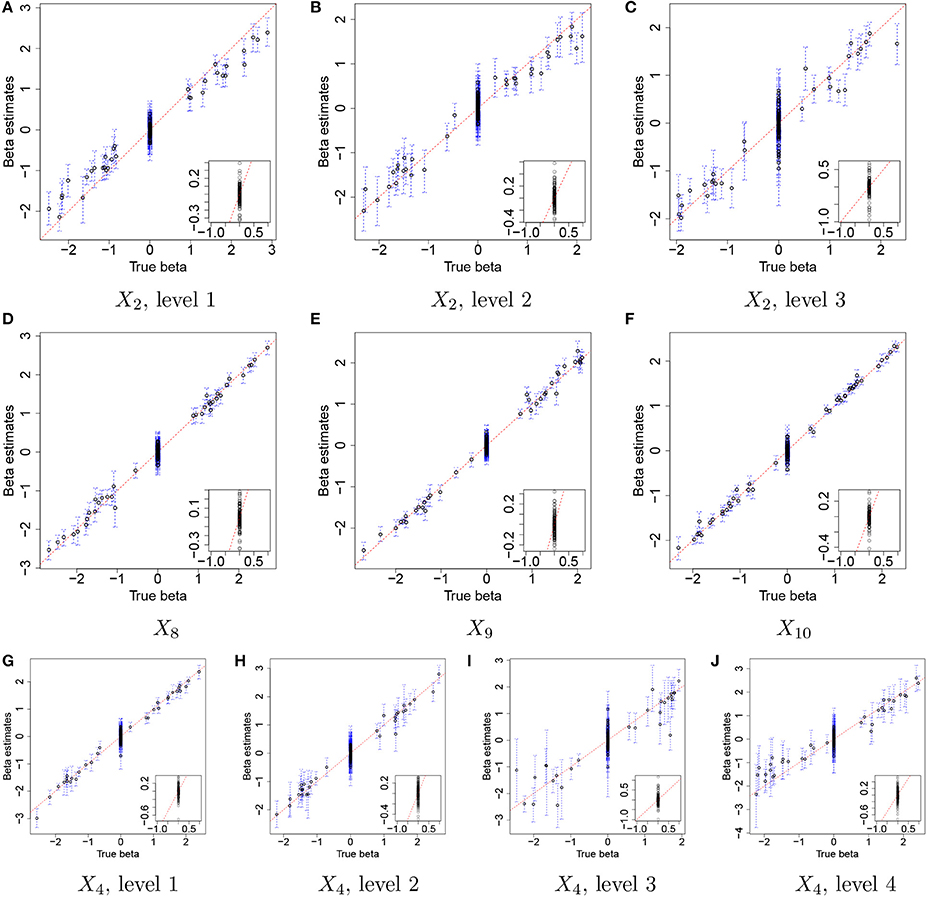
Figure 3. Simulation 1—proposed model. Comparison of the true values and the posterior estimates of βj,p under the proposed model for some selected covariates. Dots and blue dashed lines represent estimates of posterior means of βj,p and 95% credible intervals (CIs) of βj,p, respectively. The insert plot in each panel is a scatter plot of and for (j,p) with .
Figures 4A–C illustrate plots of vs estimates of gt,k,j with their means (black dots) and 95% credible intervals (blue vertical lines) for some selected OTUs, j = 8, 34, and 48. Recall that we do not attempt to recover the true values of individual rti,k, α0, j, and αt,j, but we rather aim to reasonably recover the true baseline mean counts, . In the figure the estimates are tightly around the 45 degree line, providing evidence that reasonable estimates of baseline mean counts are obtained under the proposed model. Figure 4D has a histogram of averaged differences between baseline mean count estimates and their true values, . The averaged differences are around zero, implying that the proposed model provides reasonable estimates of baseline mean counts for most of OTUs. We further examined individual parameters. Figures 4E–G shows the comparison of estimates of to their true values over time for the same OTUs in Figures 4A–C. Black dots and blue vertical lines represent estimates of posterior means of and their 95% credible intervals, respectively. Red squares represent their true values. From the figure, the estimates of are consistently greater than their true values at all time points, but capture their overall temporal trend. Figure 4H illustrates a scatterplot of and their posterior estimates of , where dots and blue vertical intervals denote estimates of posterior means and 95% credible intervals, respectively, and the gray horizontal line is at cr used for analysis. Different from the estimates of , the estimates of fall below the 45 degree line approximately by the same distance for all OTUs. It shows that estimates of and have discrepancies from their true values but in the opposite direction and the model can produce reasonable estimates of gt,k,j as seen in Figures 4A–D. The true overdispersion parameters are reasonably well estimated as shown in Figure 4I. We check the posterior predictive distribution of Yt,k,j. The posterior predicted values of Yti,k, j with their 95% predictive intervals for OTUs j = 8, 34, and 48 are compared to their observed values in Supplementary Figure 2. The figure indicates a reasonable model fit.
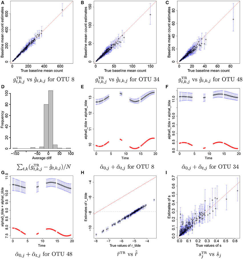
Figure 4. Simulation 1—proposed model. Panels (A–C) illustrate plots of the true baseline mean counts vs their estimates ĝt,k,j for some selected OTUs j = 8, 34, 48. Panel (D) shows a histogram of averaged differences between and ĝt,k,j for each OTU. Panels (E–G) show plots of estimates of over time for OTUs j = 8, 34, 48. Panel (H) has a scatterplot of vs. . Panel (I) has a scatterplot of ŝ vs. sTR. Dots represent posterior mean estimates and blue vertical dotted lines 95% credible intervals. Red squares represent the true values.
In addition, we conducted a sensitivity analysis to the specification of mean constraints cr and cα for the priors of and . We used different values for cr and cα and compared the estimates of gt,k,j to their truth. Supplementary Figures 3a–c has histograms of averaged differences Dj between ĝti,k, j and for different specification of cr and cα. The histograms show minor change in estimates of gti,k,j under different specifications of cr and cα. An sensitivity analysis to the specification of the number M of basis points in the GP convolution model for was also performed. We used M = 8, 13, and 18 and examined estimates of the baseline mean counts, gt,k,j. Supplementary Figures 3a,d,e has histograms of averaged differences Dj for each of M. The results indicate that the baseline mean counts are reasonably estimated for a range of values of M in the simulation study.
For comparison, we used the NBMM to the simulated data. Since the NBMM does not accommodate missing covariates, we used XTR to fit the NBMM. Figure 5 compares the MLEs of βj,p to the true values for the same covariates used in Figure 3. Dots and blue vertical lines represent the MLEs under the NBMM and their 95% confidence intervals, respectively. Comparing Figure 5 to Figure 3, the NBMM produces poor estimates. The MLEs are biased for some covariates (e.g., Figure 5A). Also, confidence intervals under the NBMM often fail to capture the true values and their interval estimates under the NBMM tend to be much wider than those under the proposed model. Normalization through observed sample total counts and inducing correlation in replicates through iid (independent and identically distributed) random effects under the NBMM may lead to poor estimation of the baseline mean abundance for the simulated data, resulting in deterioration of coefficient estimation. In addition, separate analyses of OTUs under the NBMM do not allow to strengthen estimates through combining information across OTUs. Comparing the insert plots in Figure 5 to those in Figure 3, with tends to more widely spread out from zero and often their confidence intervals fail to capture zero. Supplementary Figure 4 has plots of βj,p for all covariates. Supplementary Figures 4,5 shows the comparison of the estimates of overdispersion parameters under the NBMM to their true values. Note that θNBMM is the inverse of s in our model. The NBMM underestimates sj for many OTUs, and yields poor predicted values, implying the lack of a fit.
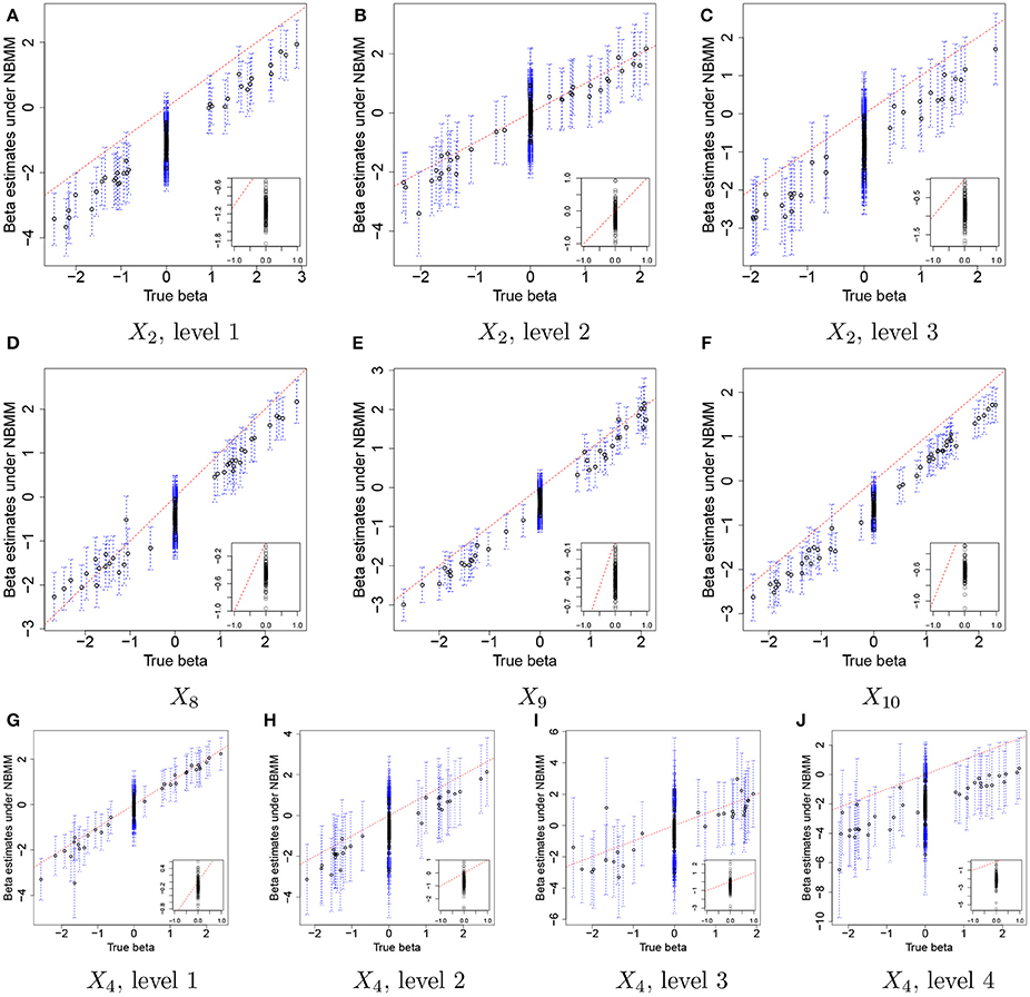
Figure 5. Simulation 1—NBMM. Comparison of the true values and maximum likelihood estimates of βj,p under the negative binomial mixed model (NBMM) for some selected covariates. Dots and blue dashed lines represent and their 95% confidence intervals, respectively. The insert plot in each panel is a scatter plot of and for (j,p) with .
We further examined the performance of the proposed model through additional simulation studies, Simulations 2 and 3 in Supplementary section 2. In these simulations, we studied the robustness of the model when different simulation setups are used to simulate data. In Simulation 2, we assumed no temporal dependence among OTU abundance and generated independent samples from a normal distribution for . We assumed that all has nonzero effects for all OTUs and simulated βj,p from a mixture of normals. The performance of our model is almost the same as in Simulation 1 (see Supplementary Figures 6–8). Interestingly, the NBMM that assumes iid random effects performs poorly for β estimation. In Simulation 3, we simulated from a discontinuous function. The results show that when the temporal dependence pattern is not smooth as assumed for the GP, estimates of the baseline mean counts under the proposed model are slightly deteriorated but the model produces reasonable inference on βj,p (see Supplementary Figures 9–11). A more detailed summary of the additional simulations is given in Supplementary section 2.
3.2. Ocean Microbiome Data: Model Fitting and Comparison
We specified hyperparameters similar to those in the simulations and analyzed the microbiome data in section 2.3. The MCMC simulation was run over 25,000 iterations. The first 15,000 iterations were discarded as burn-in and every other sample was kept as thinning and used for inference. Figure 6 illustrates inference on covariate effects for some selected OTUs, j = 16, 34, and 49, taxonomically belonging to Alteromonadales, Halomonas sp., and Alteromonadales in the Gamma-proteobacteria phyla, respectively. Dots and vertical solid lines represent the posterior mean and 95% credible interval estimates, respectively. Similar to the results of the simulation study, the credible intervals for high and highest levels of the discretized covariates tend to be wider due to their low frequencies in the data. From Figure 6A, on average the medium concentration level of domoic acid (DA, X4) and the concentration level of nitrate (N, X6) significantly decrease the mean abundance of OTU 16 by a multiplicative factor of exp(−0.572) = 0.564 and exp(−0.260) = 0.771, respectively. One may infer that the medium concentration level of domoic acid is significantly associated with lower expected counts for the OTU compared to those with category none of the domoic acid concentration level. A similar argument can be applied to the inference on the nitrate concentration level. Interestingly, we observed statistically significant reduction in abundance from many OTUs belonging to Gamma-proteobacteria including those OTUs for increasing domoic acid concentration (not shown). The resulting inference was further validated through a lab experiment. Most notably, four bacterial cultured isolates belonging to Gamma-proteobacteria (three among them are Alteromonadales) were observed to be severely retarded in growth after 2 days of exposure to increasing domoic acid of 0 to 150 μg/ml in the experiment (Sison-Mangus, unpublished data). This demonstrates that the proposed model successfully identifies important OTUs in ocean bacterial community dynamics for further investigation. More results are presented in Supplementary Section 3. Supplementary Figures 12a–c illustrates the posterior estimates of baseline expected counts normalized by sample size factors for the OTUs. From the figure, the baseline expected counts vary over time for those OTUs and the temporal pattern of OTU j = 34 is different from those of OTUs j = 16 and 49. Histograms of the posterior mean estimates of βj,p, are illustrated in Supplementary Figure 13. The figure does not show clear overall tendency in the direction of association between covariates and OTU counts. Posterior inference on sample size factors rti,k and OTU specific overdispersion parameters sj is illustrated in Supplementary Figures 12d,e.
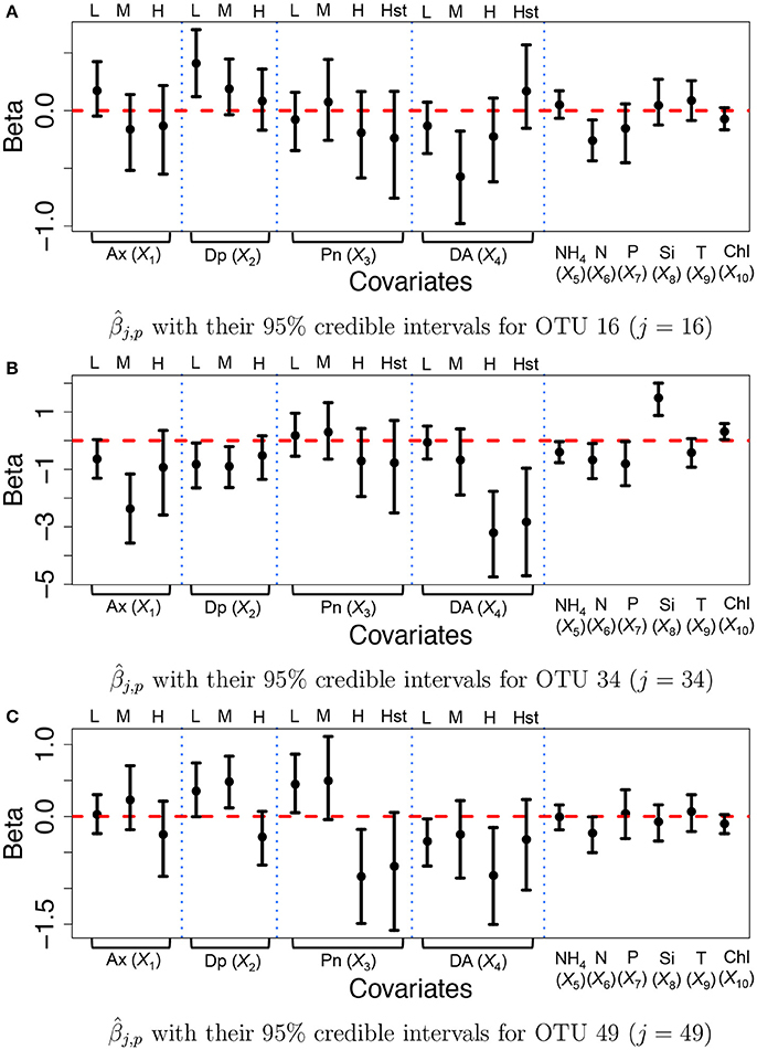
Figure 6. Ocean microbiome data—proposed model. Posterior Inference on βj for some selected OTUs (j = 16, 34, 49). Dots represent the posterior means of βj,p. Each vertical line connects the lower bounds and the upper bounds of 95% credible intervals.
For comparison, we fitted the NBMM to the data. Since the NBMM does not account for missing values, we use the maximum a posteriori estimates of the missing values under the proposed for the NBMM. We used the R function glmm and the algorithm produced warning messages on convergence for 32 OTUs. Figure 7 illustrates (dots) with their 95% confidence intervals (solid vertical lines) for OTUs j = 16, 34, and 49. Inference on the covariate effects is different from that under the proposed. For example, domoic acid (DA) levels do not have significant effects on the mean counts for OTU j = 16 and 49 from Figures 7A,C. Comparing Figures 7A,C to Figure 7, the NBMM produces wider interval estimates for βj,p. Histograms of the MLEs of βj,p, under the NBMM are shown in Supplementary Figure 14. The histograms are much dispersed than those under the proposed model shown in Supplementary Figure 13. Estimates and for all covariates are also compared in Supplementary Figure 15. From the figure, the NBMM yields extremely large or small values for for some OTUs, possibly due to the convergence problem. The insert plots show that for regions of small values of , the estimates under the proposed are more shrunken toward zero than those under the NBMM, similar to the results in section 3.1. The overdispersion parameter estimates under the NBMM tend to be smaller than those under the proposed (shown in Supplementary Figure 12f), which may lead to different predictive distributions of OTU counts.
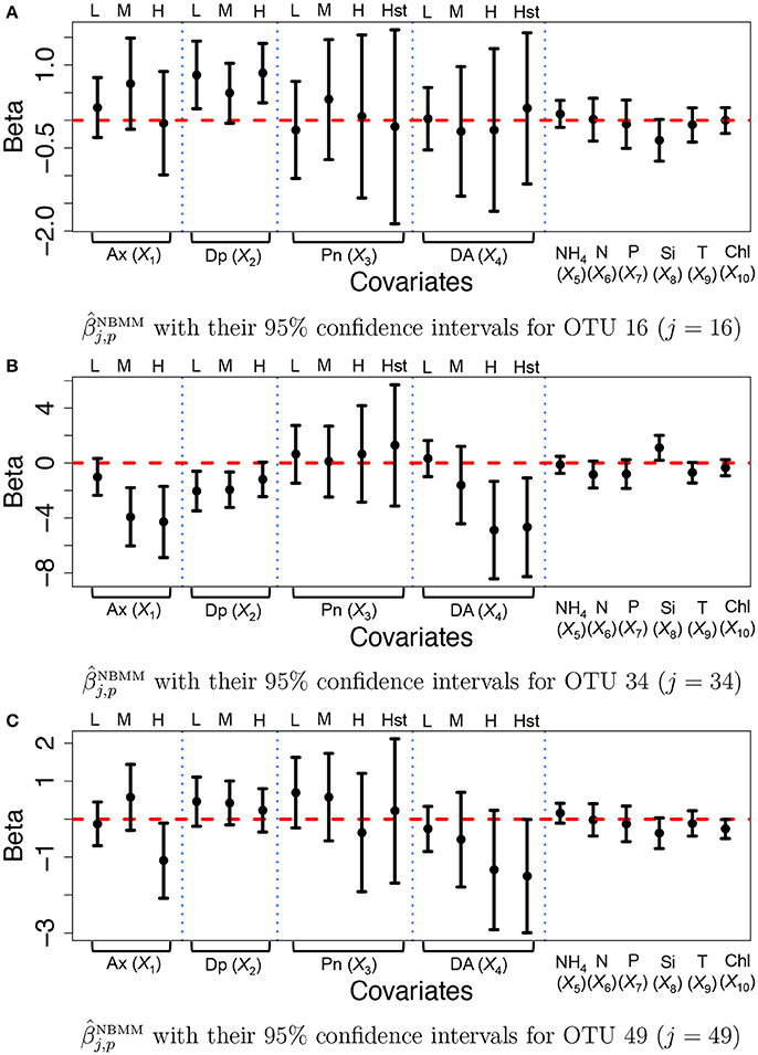
Figure 7. Ocean microbiome data—NBMM. Inference on βj for some selected OTUs (j = 16, 34, 49) under the negative binomial mixed model (NBMM). Dots represent the maximum likelihood estimates of βj,p. Each vertical line connects the lower bounds and the upper bounds of 95% confidence intervals.
4. Discussion and Conclusions
In this paper, we developed a Bayesian semiparametric regression model for joint analysis of microbiome data. We formulated the mean counts of OTUs as a product of factors and built models for the factors. We utilized the regularizing priors with mean constraints to avoid possible idenfiability issues, and the process convolution model to capture the temporal dependence structure in the baseline mean abundance of an OTU. The flexible model developed for baseline abundance enables joint analysis of all OTUs in the data and allows borrowing information across OTUs, across samples, and across time points. The model produces accurate estimates of the baseline mean counts and yields improved estimates of the effects of the covariates. We incorporated the Laplace distribution, a sparsity inducing shrinkage prior for the coefficients and the proposed model produces sparse estimates that is more desirable when the problem is high-dimensional and covariates are highly correlated. We compared the proposed model to a comparable frequentist model that does separate analyses for individual OTUs. The comparisons through the simulation study and real data analysis show better performance of the proposed model.
Although we focused on the analysis of NGS count data, the proposed model is quite general and can be applied for analyses of any count data. Future work will explore alternative approaches to model the effects of covariates on the mean counts. For example, one may consider a nonparametric model using linear combinations of basis functions (Kohn et al., 2001) to flexibly capture shape in the response function. In such a case, an elaborate development of the prior model may be needed to produce a robust inference since both the baseline mean counts and the covariate effects are nonparametrically modeled. Other possible extensions are to include a variable selection method such as a stochastic search variable selection (George and McCulloch, 1993) if it is reasonable to assume that some covariate effects are exactly zero, and to let coefficients vary over time if covariate effects evolve with time. For time varying coefficients, we may use the random walk process in Leybourne (1993) to induce relationship between βj,p,t−1 and βj,p,t. Considering the high dimensionality in OTU data, posterior computation may need to be carefully handled. Also, prior information may be needed to produce sensible inference due to sparsity in data.
Author Contributions
JL developed the statistical model and conducted simulation studies and data analysis. She also prepared the first draft and led the collaboration with MS-M for statistical analysis. MS-M provided the ocean microbiome data, participated the statistical model development, provided biological interpretation of the resulting inference and edited the manuscript.
Funding
This work was supported by NSF grant DMS-1662427 (JL) and NOAA-ECOHAB PROGRAM (Grant No. NA17NOS4780183, ECOHAB #905) (MS-M and JL). Collection of environmental data from the Santa Cruz Municipal Wharf was supported by Cal-PReEMPT with funding from the NOAA-MERHAB (#206), ECOHAB and IOOS programs.
Conflict of Interest Statement
The authors declare that the research was conducted in the absence of any commercial or financial relationships that could be construed as a potential conflict of interest.
Acknowledgments
We gratefully acknowledge Raphael Kudela who provided the environmental data in this study, Michael Kempnich and Sanjin Mehic for doing the water sampling and processing the water samples for DNA extraction.
Supplementary Material
The Supplementary Material for this article can be found online at: https://www.frontiersin.org/articles/10.3389/fmicb.2018.00522/full#supplementary-material
References
Anders, S., and Huber, W. (2010). Differential expression analysis for sequence count data. Genome Biol. 11:R106. doi: 10.1186/gb-2010-11-10-r106
Banerjee, S., Carlin, B. P., and Gelfand, A. E. (2014). Hierarchical Modeling and Analysis for Spatial Data. 2nd Edn. Boca Raton, FL: CRC Press; Chapman & Hall.
Chen, E. Z., and Li, H. (2016). A two-part mixed-effects model for analyzing longitudinal microbiome compositional data. Bioinformatics 32, 2611–2617. doi: 10.1093/bioinformatics/btw308
George, E. I., and McCulloch, R. E. (1993). Variable selection via gibbs sampling. J. Am. Stat. Assoc. 88, 881–889.
Gibbons, S. M., Kearney, S. M., Smillie, C. S., and Alm, E. J. (2017). Two dynamic regimes in the human gut microbiome. PLoS Comput. Biol. 13:e1005364. doi: 10.1371/journal.pcbi.1005364
Higdon, D. (1998). A process-convolution approach to modelling temperatures in the north atlantic ocean. Environ. Ecol. Stat. 5, 173–190.
Higdon, D. (2002). “Space and space-time modeling using process convolutions,” in Quantitative Methods for Current Environmental Issues, eds C. W. Anderson, V. Barnett, P. C. Chatwin, and A. H. El-Shaarawi (London: Springer), 37–56.
Kohn, R., Smith, M., and Chan, D. (2001). Nonparametric regression using linear combinations of basis functions. Stat. Comput. 11, 313–322. doi: 10.1023/A:1011916902934
Leybourne, S. J. (1993). Estimation and testing of time-varying coefficient regression models in the presence of linear restrictions. J. Forecast. 12, 49–62.
Lee, H. K., Higdon, D. M., Calder, C. A., and Holloman, C. H. (2005). Efficient models for correlated data via convolutions of intrinsic processes. Stat. Model. 5, 53–74. doi: 10.1191/1471082X05st085oa
Li, Q., Guindani, M., Reich, B., Bondell, H., and Vannucci, M. (2017). A bayesian mixture model for clustering and selection of feature occurrence rates under mean constraints. Stat. Anal. Data Mining 10, 393–409. doi: 10.1002/sam.11350
Liang, W. W., and Lee, H. K. (2014). Sequential process convolution gaussian process models via particle learning. Stat. Interface 7, 465–475. doi: 10.4310/SII.2014.v7.n4.a4
McCullagh, P., and Nelder, J. A. (1989). Generalized Linear Models, No. 37 in Monograph on Statistics and Applied Probability. Boca Raton, FL: Chapman & Hall/CRC.
McMurdie, P. J., and Holmes, S. (2014). Waste not, want not: why rarefying microbiome data is inadmissible. PLoS Comput. Biol. 10:e1003531. doi: 10.1371/journal.pcbi.1003531
Needham, D. M., and Fuhrman, J. A. (2016). Pronounced daily succession of phytoplankton, archaea and bacteria following a spring bloom. Nat. Microbiol. 1:16005. doi: 10.1038/nmicrobiol.2016.5
Park, T., and Casella, G. (2008). The bayesian lasso. J. Am. Stat. Assoc. 103, 681–686. doi: 10.1198/016214508000000337
Polson, N. G., and Scott, J. G. (2012). Local shrinkage rules, lévy processes and regularized regression. J. R. Stat. Soc. Ser. B 74, 287–311. doi: 10.1111/j.1467-9868.2011.01015.x
Robinson, M. D., and Smyth, G. K. (2007). Moderated statistical tests for assessing differences in tag abundance. Bioinformatics 23, 2881–2887. doi: 10.1093/bioinformatics/btm453
Romero, R., Hassan, S. S., Gajer, P., Tarca, A. L., Fadrosh, D. W., Nikita, L., et al. (2014). The composition and stability of the vaginal microbiota of normal pregnant women is different from that of non-pregnant women. Microbiome 2:4. doi: 10.1186/2049-2618-2-4
Sison-Mangus, M. P., Jiang, S., Kudela, R. M., and Mehic, S. (2016). Phytoplankton-associated bacterial community composition and succession during toxic diatom bloom and non-bloom events. Front. Microbiol. 7:1433. doi: 10.3389/fmicb.2016.01433
Turnbaugh, P. J., Hamady, M., Yatsunenko, T., Cantarel, B. L., Duncan, A., Ley, R. E., et al. (2009). A core gut microbiome in obese and lean twins. Nature 457, 480–484. doi: 10.1038/nature07540
Witten, D. M. (2011). Classification and clustering of sequencing data using a poisson model. Ann. Appl. Stat. 5, 2493–2518. doi: 10.1214/11-AOAS493
Woo, P., Lau, S., Teng, J., Tse, H., and Yuen, K.-Y. (2008). Then and now: use of 16s rDNA gene sequencing for bacterial identification and discovery of novel bacteria in clinical microbiology laboratories. Clin. Microbiol. Infect. 14, 908–934. doi: 10.1111/j.1469-0691.2008.02070.x
Xiao, S. (2015). Bayesian Nonparametric Modeling for Some Classes of Temporal Point Processes. Ph.D. thesis, University of California, Santa Cruz.
Keywords: count data, Laplace prior, metagenomics, microbiome, regularizing prior, process convolution, negative binomial model, 16S ribosomal RNA sequencing
Citation: Lee J and Sison-Mangus M (2018) A Bayesian Semiparametric Regression Model for Joint Analysis of Microbiome Data. Front. Microbiol. 9:522. doi: 10.3389/fmicb.2018.00522
Received: 15 November 2018; Accepted: 08 March 2018;
Published: 26 March 2018.
Edited by:
Michele Guindani, University of California, Irvine, United StatesReviewed by:
Yanxun Xu, Johns Hopkins University, United StatesMichael Pester, Deutsche Sammlung von Mikroorganismen und Zellkulturen (DSMZ), Germany
Copyright © 2018 Lee and Sison-Mangus. This is an open-access article distributed under the terms of the Creative Commons Attribution License (CC BY). The use, distribution or reproduction in other forums is permitted, provided the original author(s) and the copyright owner are credited and that the original publication in this journal is cited, in accordance with accepted academic practice. No use, distribution or reproduction is permitted which does not comply with these terms.
*Correspondence: Juhee Lee, juheelee@soe.ucsc.edu