A reinforcement learning model of precommitment in decision making

Introduction

Precommitment is a general mechanism to control impulsive behavior (Ainslie, 1975, 2001; Dripps, 1993). An alcoholic trying to quit may decide to avoid going to the bar, knowing that if he goes, he will drink. By avoiding the bar, he precommits to the decision of not drinking. Similarly, a heroin addict may take methadone even though it will preclude the euphoria of heroin. In general, precommitment is an action that alters the external environment (in the methadone example, the external environment includes the neuropharmacology of the individual) to foreclose the possibility of a future impulsive choice. It is important to note that precommitment is not synonymous with self-control: self-control entails an act of willpower to avoid an impulsive choice; precommitment strategies actually constrain the agent’s future choices. The strategy of precommitment is ubiquitous in decision-making outside of addiction as well. Putting the ice cream out of sight, investing money in an inaccessible retirement fund, and pre-paid gym memberships can be precommitment devices.

Precommitment devices combat impulsivity, the overvaluation of immediate rewards relative to delayed rewards¹. To describe impulsivity quantitatively, we use the generalized notion of delay discounting, the decrease in subjective value associated with rewards that are more distant in the future (Koopmans, 1960; Fishburn and Rubinstein, 1982; Mazur, 1987; Madden and Bickel, 2010). A discounting function specifies how much less subjective value a reward has at any given time in the future. An individual’s discounting function can be inferred from choices. For example, if a subject prefers $20 in a week equally to $10 today, then the subject discounts by 50% over that one week. Drug addicts discount faster than non-addicts (Madden et al., 1997; Bickel et al., 1999; Coffey et al., 2003; Dom et al., 2006). Thus one potential driver for addiction is that an addict may prefer a small immediate reward (drugs) over a large delayed reward (academic and career success, family, health, etc.). The ability to precommit is especially valuable when impulsive behavior is leading to serious problems such as drug abuse.

If each unit of time by which the reward is delayed causes the same attenuation of the reward’s value, then discounting is exponential. In other words, the subjective value is attenuated by γ^d, where d is the delay to the reward, and γ is the amount of attenuation incurred by each unit of time. Exponential discounting is theoretically optimal in certain situations (Samuelson, 1937) and can be calculated recursively (Bellman, 1958; Sutton and Barto, 1998). Exponential discounting also has the property that two rewards separated by a given delay will maintain their relative values whether they are considered well in advance or they are near at hand. However, behavioral studies show that humans and animals do not discount exponentially; real discounting is usually better fit by a hyperbolic function (Ainslie, 1975; Madden and Bickel, 2010). In hyperbolic discounting, subjective value is attenuated by , where d is again the delay to reward, and k determines the steepness of the hyperbolic curve.

An agent using hyperbolic discounting will exhibit preference reversal (Strotz, 1955; Ainslie, 1992; Frederick et al., 2002). As the time at which a choice is considered changes, the preference order reverses. For example, the agent may prefer to receive $10 today over $15 in a week, but prefer $15 in 53 weeks over $10 in 52 weeks. Humans and animals consistently display preference reversal (Madden and Bickel, 2010). In fact, preference reversal is not exclusive to hyperbolic discounting. If discounting consists of a function that maps delay to an attenuation of subjective value, then exponential decay is the only discounting function in which preference reversal does not appear.

It has been suggested that preference reversal is the basis for precommitment (Ainslie, 1992). Preference reversal entails a conflict between current (non-impulsive) and future (impulsive) preferences. This conflict leads the individual to commit to current preferences, to prevent the future self from undermining these preferences. For example, in 52 weeks, the agent will be given a choice between $10 then or $15 a week from then. If that choice is made freely, he will choose the $10. Because he presently prefers the $15, he may enter now into a contract that binds him to choosing the $15 option when the choice becomes available.

To explicitly test whether precommitment can be learned in a controlled setting, Rachlin and Green (1972) and Ainslie (1974) trained pigeons on tasks that required choosing between smaller-sooner and larger-later options. After learning this paradigm, the pigeons were given an option preceding this choice, to inactivate the smaller-sooner option. Some pigeons that preferred smaller-sooner over larger-later would nonetheless elect to inactivate the smaller-sooner option – thereby precommitting to the larger-later option. The pigeons’ willingness to precommit increased with the delay between precommitment and choice.

Here we develop a quantitative theory of how such precommitment may occur, based on reinforcement learning. Precommitment has not previously been implemented in a reinforcement learning model. Four models have been proposed to explain how a biological learning system could plausibly calculate hyperbolic discounting. First, in the average reward model (Tsitsiklis and Van Roy, 1999; Daw and Touretzky, 2000; Dezfouli et al., 2009), discounting across states is linear (i.e., each additional unit of delay subtracts a constant from the subjective value), but the slope of this linear discounting is set, based on the reward magnitude, such that the total discounting over d delay is . An average reward variable keeps track of the slope so that it is available for the linear discounting calculation at each state. Second, in a variant of the average reward model (Alexander and Brown, 2010), if R is the average reward per trial and V is the value after d delay, then the value after d + 1 delay is calculated as VR/(V + R). This produces hyperbolic discounting across states, given a linear state-space (i.e., a chain of states with no branches or choices) leading to a reward. The third method of calculating hyperbolic discounting is semi-Markov state representations, where a variable amount of time can elapse while the agent dwells within a single state (Daw, 2003). The agent can simply compute the hyperbolic discount factor (1/(1 + d)) over the entire duration, d, of the state. In the fourth model, exponential discounting is performed in parallel at various rates by a set of reinforcement learning “μAgents,” who collectively form the decision-making system of the overall agent (Kurth-Nelson and Redish, 2009). In the μAgents model, choices of the overall agent are derived by taking the average value belief over the set of μAgents. Averaging across a set of different exponential discount curves yields a good approximation of hyperbolic discounting (e.g., Sozou, 1998) that functions over multiple state transitions.

In this paper we first show that, of the four available hyperbolic discounting models, only the μAgents model can precommit. We then use the μAgents model to test specific predictions about the properties of precommitment behavior. Understanding the basis of precommitment may help to create situations where precommitment will be successful in the treatment of addiction as well as inform the study of decision-making in general.

Materials and Methods

We compare four models in this paper. Each model is an implementation of temporal difference reinforcement learning (TDRL) (Sutton and Barto, 1998). Each model consisted of a simulated agent operating in an external world. The agent performed actions that influenced the state of the world, and in certain states the world supplied rewards to the agent. The available states of the world, together with the set of possible transitions between states, formed a state-space. Each state i was associated with a number R(i) (which may be 0) specifying how much reward the agent received upon leaving that state. In semi-Markov models, each state was also associated with a delay specifying the temporal extent of the state (how long the agent must wait before receiving the reward and/or transitioning to another state) (Daw, 2003). In fully-Markov models, each state had a delay of one time unit, so variable delays were modeled by increasing or decreasing the number of states.

The agent learned, for each state, the total expected future reward from that state, discounted by the delay to reach that reward (or rewards). This discounted expected future reward is called value. The value of state i is called V(i). Learning these values allowed the agent, faced with a choice between two states, to choose the state that would lead to more total expected reward².

The parameter values used in the simulations are listed in Table 1.

TABLE 1

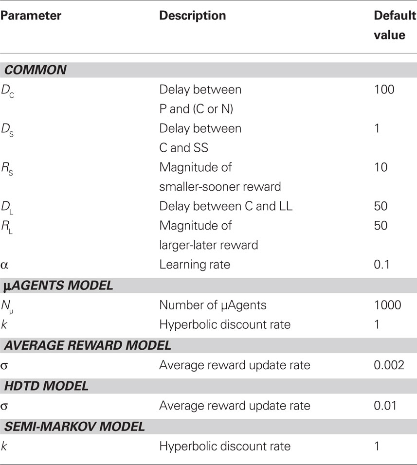
Table 1 Parameters used in the model (except where noted otherwise).

μAgents Model

The μAgents model is described in detail in Kurth-Nelson and Redish (2009). The model produces identical behavior (including precommitment) in semi-Markov or fully-Markov state-spaces.

In the μAgents model, the agent (which we will sometimes call “macro-agent” for clarity) consisted of a set of μAgents, each performing TDRL independently. For a given state, different μAgents could learn different values. To select actions, the different values across μAgents were averaged. The only difference between μAgents was that each μAgent had a different discount rate.

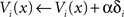
Upon each state-transition from state x to state y, each μAgent i generated an error signal, δ_i, reflecting the discrepancy between (discounted) value observed and value predicted:

where V_i(x) is the value of state x learned by μAgent i, γ_i is the discount rate of μAgent i, and d is the delay spent in state x. Note that the total benefit of moving from state x to state y is the reward received (R(x)) plus the reward expected in the future of the new state (V_i(y)). Because future value is attenuated by a constant multiple (γ_i) for each unit of delay, the discounting of each μAgent is exponential. The values of γ were spread uniformly over the interval: [1/(N_μ + 1), 1 − 1/(N_μ + 1)], where N_μ is the number of μAgents. Thus if there were nine μAgents, they would have discount rates 0.1, 0.2, 0.3, 0.4, 0.5, 0.6, 0.7, 0.8, and 0.9.

To improve value estimates, each μAgent i used the error signal to update its V_i(x) after each state-transition:

where α is a learning rate in (0,1) common to all μAgents. α = 0.1 was used in all simulations.

From some states, actions were available to the macro-agent. Let A be the set of possible actions. Since each action in our simulations leads to a unique state, A is equivalently a set of states. The probability of selecting action a∈A was:

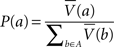
where denotes the average value of state a across μAgents. Note that the probabilities sum to one across the set of available actions; exactly one action from A was chosen.

Because each μAgent had an independent discount rate, this model is considered to perform distributed discounting. One consequence of distributed discounting is that although each individual μAgent performs exponential discounting, the overall discounting produced by the macro-agent approaches hyperbolic as the number of μAgents increases:

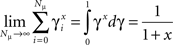
when hyperbolic discounting is implemented as a sum of exponentials, it is hyperbolic across multiple state transitions. For more details on how distributed exponential discounting produces hyperbolic discounting, see Kurth-Nelson and Redish (2009). In this model we were also able to adjust the effective hyperbolic parameter k by biasing the distribution of μAgent exponential discount rates (γ) (Kurth-Nelson and Redish, 2009).

Average Reward Model

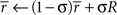
The average reward model (Tsitsiklis and Van Roy, 1999; Daw and Touretzky, 2000; Dezfouli et al., 2009) uses a fully-Markov state-space. A variable tracked the average reward per timestep:

where R was the reward received on this timestep, and σ controlled the rate at which changed. The reward prediction error δ, upon transition from state x to state y, was calculated as:

This produced linear discounting, because the value of x approached the value of y minus (which is effectively a constant because σ is very small). In a linear state space with d′ delay leading to R′ reward, would approach where (1 + d′) is the total length of a trial, including one time step to receive the reward), which is hyperbolic discounting as a function of total delay. In other words, the average reward model discounts linearly across a given state-space, but the total discounting across this state space is hyperbolic because the linear rate depends on the total delay of the state-space. The average reward model does not show hyperbolic discounting in a state-space with choices (branch points), because no longer approaches .

HDTD Model

The HDTD model (Alexander and Brown, 2010) also uses a fully-Markov state-space. In this model, average reward is tracked per trial rather than per timestep, but using the same update rule as the average reward model:

The reward prediction error was calculated as:

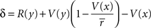
In a linear state space with d′ delay leading to R′ reward, would approach R'. Through algebra, V(x) would approach:

which would produce hyperbolic discounting across states. In other words, in a linear chain of states, the value of a state is attenuated as a hyperbolic function of the temporal distance from that state to the reward. The HDTD model does not show hyperbolic discounting in a state-space with choices (branch points), because no longer approaches R′.

Semi-Markov Model

The semi-Markov model is a standard temporal difference reinforcement learning model in a semi-Markov state-space (Daw, 2003). This model was identical to μAgents, except there was only a single reinforcement learning entity, and it used the following rule instead of Eq 1:

where again k is the discount rate (set to 1 for these simulations), and d is the delay spent in state x before transitioning to state y.

Results

We ran the μAgents model on the precommitment state-space illustrated in Figure 1. The states and transitions inside the dashed box represent a simple choice between a smaller reward (R_S) available after a short delay (D_S) and a larger reward (R_L) available after a long delay (D_L). We will refer to the smaller-sooner choice as SS and the larger-later choice as LL. C was the state from which this choice is available. Although R_L was a larger reward than R_S, SS could be the preferred choice if D_S was sufficiently shorter than D_L, due to temporal discounting of future rewards.

FIGURE 1

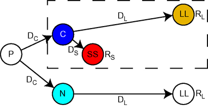
Figure 1. A reinforcement learning state-space with an option to precommit to a larger-later reward. This is the task on which the model was run. Time is schematically portrayed along the horizontal axis. The dashed box encloses the state-space for a simple two-alternative choice. From state C, the agent could choose a large reward R_L following a long delay D_L, or a small reward R_S following a short delay D_S. Preceding this simple choice was the option to precommit. From state P, the agent could either enter the simple choice by choosing C, or to precommit to the large delayed choice by choosing N. A precommitment delay D_C separated P from the subsequent state.

Over the course of learning, each μAgent independently approached a steady-state estimate of the correct exponentially discounted value of each state. When values were fully learned, , and for a given μAgent i. Thus, the value estimates averaged across μAgents approximated the hyperbolically discounted values:

and

At state C, if the agent always selected SS, then the value of C would approach the discounted value of SS. Since the agent sometimes selected LL, the actual value of C was between the discounted values of SS and LL. The steady-state value of state C, for a given μAgent i, was:

where is the probability of selecting SS from C, and is the probability of selecting LL from C. Thus, the average value of the C state approximated

Precommitment can be defined as limiting one’s future options so that only the pre-selected option is available. This is represented in Figure 1 by the state P which precedes the SS vs. LL choice. At state P, a choice was available to either enter the SS vs. LL choice, or to enter a situation (state N) from which only the LL option was available. In either case, there was a delay D_C following the choice made at state P.

The value of state N, averaged across μAgents, approximated

in the steady-state. By definition, the macro-agent preferred to precommit if and only if .

μAgents Model Precommits

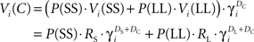
We examined choice behavior in the model, using a specific set of parameters designed to simulate the choice between a small reward available immediately (R_S = 10, D_S = 1) and a large reward available later (R_L = 50, D_L = 50). The discounting rate k was set to 1. The number of μAgents, N_μ, was set to 1000. The preference of the model was measured from the choices made at steady-state (after learning). Using these parameters, the model preferred SS over LL by a ratio of 5.2:1 (Figure 2A).

FIGURE 2

Figure 2. The μAgents model exhibited precommitment behavior. (A) From P, the model chose N more often than C. However, when C was reached, the model chose SS more often than LL. This bar graph represents the same data as (B) at R_S = 10. (B) plots the same information as (A), over a range of values of R_S. For very small R_S, LL > SS and N > C. For very large R_S, SS > LL, and C > N. However, precommitment could occur because SS crossed LL at a different point than C crossed N, meaning that there was a range of R_S for which SS > LL and N > C. (C) illustrates the change in the average value of each option over time. The distributed value representation of μAgents allowed average values to cross. The value of C prior to discounting across the D_C interval was between the discounted values of SS and LL, and was therefore above N. However, during the D_C interval, the value of C crossed under N, such that N > C at the time of the C/N choice. Note that (C) uses a fully Markov state-space to show how values are discounted through each intermediate time point. Each circle shows the value of one state after values are fully learned.

We also looked at the precommitment behavior of the model; that is, the preference of the model for the N state over the C state. The precommitment delay, D_C, was set to 100. Choices were again counted after the model had reached steady-state. Despite a strong preference for SS over LL, the model also exhibited a preference for N over C, by a ratio of 2.3:1 (Figure 2A). It is interesting to note that each μAgent that prefers SS over LL also prefers C over N (and vice versa), yet the system as a whole can prefer SS over LL while preferring N over C.

Thus, the model precommitted to LL even though SS was strongly preferred over LL. This shows that precommitment can occur for particular task parameters. We next varied the small reward magnitude, R_S, to see in what range precommitment was possible (Figure 2B). If R_S was very small, then SS was not valuable and LL was preferred over SS. If R_S was very large, the model would not precommit because the SS choice was too valuable. However, there was a range of R_S where SS was preferred over LL but N was preferred over C. This range was where the model would choose to precommit to avoid an impulsive choice. Note that in this graph we have manipulated only R_S for convenience; similar plots can be generated by manipulating any of these task parameters: R_S, D_S, R_L, and D_L.

To illustrate how precommitment arose in the μAgents model, we ran the model on a fully-Markov version of the precommitment state-space (Figure 2C). Here, each state corresponds to a single time-step, so a delay is represented by a chain of states. Each circle represents the average value of one state. First, note that the values of states in the LL and N chains overlapped because they were the same temporal distance from the same reward (R_L). The last state in the C chain necessarily had a value intermediate to the first states in the SS and LL chains³. Thus, if SS was preferred to LL, then the last state in the C chain must have a value above the corresponding state in the N chain. This means that if there was no delay D_C, C would be preferred to N. However, during the delay D_C, the C chain crossed under the N chain. This was possible because the μAgents collectively maintain a distribution of values for each state (which is collapsed to a single average value for the sake of action selection). The same average value can come from different distributions. In particular, the last state in the C chain had more value concentrated in the fast-discounting μAgents (because of the contribution from SS), while the corresponding state in the N chain had more value concentrated in the slow-discounting μAgents. Thus more of the value in the C chain was attenuated by the delay D_C, allowing N to be preferred to C.

Note that in the limit as the number of μAgents goes to infinity and the learning rate α goes to 0, the choice behavior of the μAgents model (including precommitment) becomes analytically equivalent to “mathematical” hyperbolic discounting. For example, Figure 8A compares the precommitment behavior produced by either mathematical hyperbolic discounting or 1000 μAgents. In mathematical hyperbolic discounting, the value of each choice is calculated by the right-hand side of Eqs. 2–5. This produces “sophisticated” decision-making (O’Donoghue and Rabin, 1999), because the value of C is influenced by the relative probability of selecting SS vs. LL.

Other Hyperbolic Discounting Models cannot Precommit

We investigated the behavior of three other models of hyperbolic discounting on the precommitment task. None of these models produce precommitment behavior, because they do not correctly implement hyperbolic discounting across two choices. In general, it is impossible to precommit (where precommitment is defined, using the state-space given in this paper, as preferring N over C while also preferring SS over LL) with temporal difference learning if we make the assumption that discounting preserves order (i.e., if x₁ is greater than x₂, then x₁ discounted by d delay is greater than x₂ discounted by the same d delay). Prior to discounting across the D_C interval, V(C) lies between V(SS) and V(LL), while V(N) is equal to V(LL). Thus the undiscounted V(C) is greater than the undiscounted V(N) if and only if V(SS) > V(LL). But both V(C) and V(N) are discounted by D_C. Assuming discounting preserves order, then V(C) > V(N) ⇔V(SS) > V(LL).

Note that precommitment is possible in the μAgents model because the assumption that discounting preserves order is violated. Value is represented as a distribution across μAgents, so it is possible that the average undiscounted value of V(C) is greater than the average undiscounted value of V(N), but after discounting both distributions by the same delay, the average value of V(C) is less than the average value of V(N).

We implemented the average reward model of hyperbolic discounting (Tsitsiklis and Van Roy, 1999; Daw and Touretzky, 2000; Dezfouli et al., 2009). In this model, when SS was preferred to LL, C was also preferred to N (Figures 3A,B). Although discounting as a function of total delay is hyperbolic in this model, the discounting from state to state is approximately linear (Figure 3C). The value of the last state in the C chain is between the discounted values of SS and LL, and this value is greater than the value of the corresponding state in the N chain (provided that SS is preferred to LL). Unlike in the μAgents model, the C and N chains never cross, so C is preferred to N at the time of the C/N choice (Figure 3C). The average reward model fundamentally fails to precommit because it only produces hyperbolic discounting across a linear state-space. When the state-space includes choices (branch points), discounting is no longer hyperbolic.

FIGURE 3

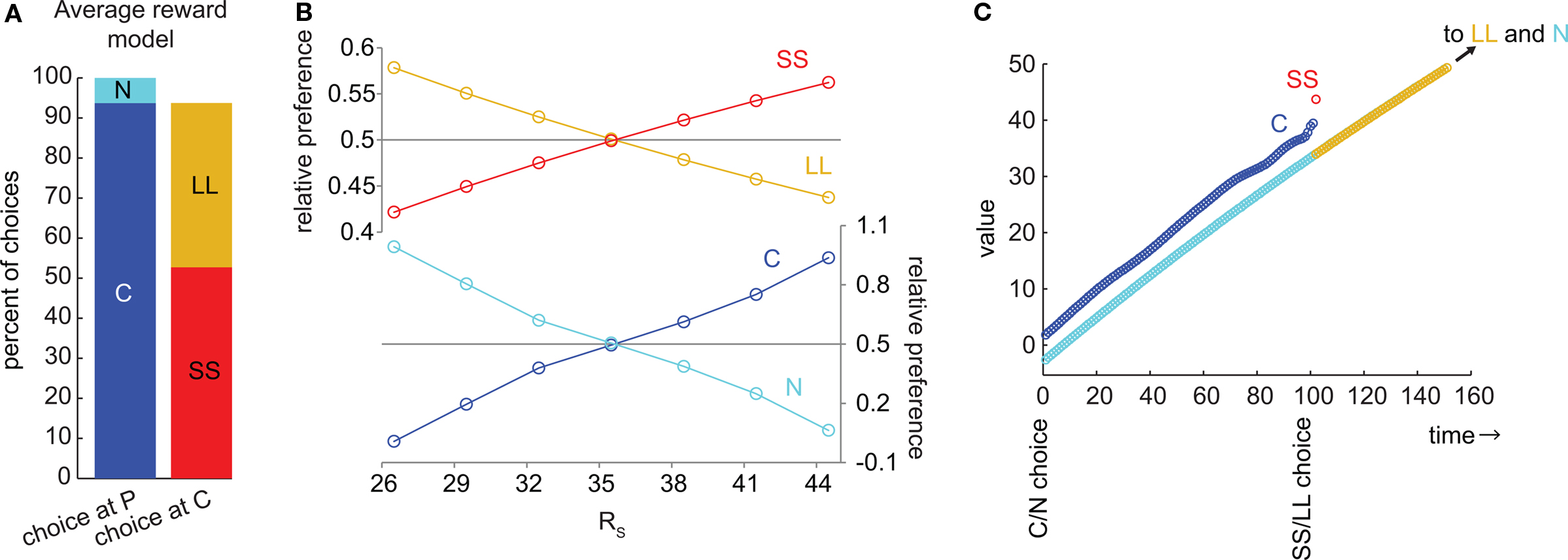
Figure 3. The average reward model of hyperbolic discounting cannot produce precommitment behavior. (A) At the selected parameters, SS was preferred to LL and C was preferred to N. This bar graph represents the same data as (B) at R_S = 44.5. (B) As R_S increased, the preference for C overtook N exactly at the same point as the preference for SS overtook LL, meaning that this model would not precommit to avoid an impulsive choice. (C) In the average reward model, the undiscounted value of C is again between the discounted values of SS and LL. However, the values of C and N never cross, so C is preferred to N whenever SS is preferred to LL. Note that discounting across states in this model is approximately linear.

The HDTD model (Alexander and Brown, 2010) is a variant of the average reward model which allows for hyperbolic discounting from state to state. Like the average reward model, HDTD preferred C to N whenever it preferred SS to LL (Figures 4A,B). Like the average reward model, the C and N chains never cross (Figure 4C), so if SS is preferred to LL, then C is preferred to N. Again, the reason the HDTD model cannot precommit is that it only produces hyperbolic discounting across a linear state-space. Both the average reward and HDTD models use an “average reward” variable to violate the Markov property, altering the discount rate based on the delay to reward. Because there is only a single “average reward” variable in each model, this mechanism works only when there is a single reward to track the delay to.

FIGURE 4

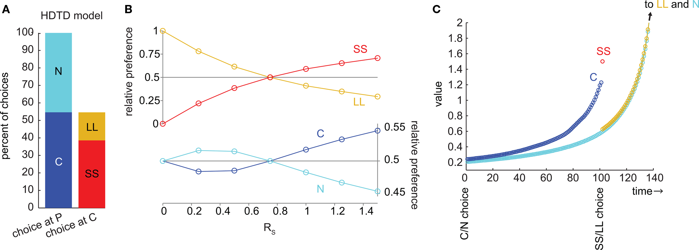
Figure 4. The HDTD model of hyperbolic discounting cannot produce precommitment behavior. (A) At the selected parameters, SS was preferred to LL and C was preferred to N. This bar graph represents the same data as (B) at R_S = 1.5. (B) As R_S increased, the preference for C overtook N exactly at the same point as the preference for SS overtook LL, meaning that this model would not precommit to avoid an impulsive choice. (C) In the HDTD model, the undiscounted value of C is between the discounted values of SS and LL. However, the values of C and N never cross, so C is preferred to N whenever SS is preferred to LL.

We also tested a semi-Markov model without distributed discounting (Daw, 2003). This model did not exhibit precommitment behavior (Figures 5A,B). Whenever SS was preferred to LL, C was preferred to N.

FIGURE 5

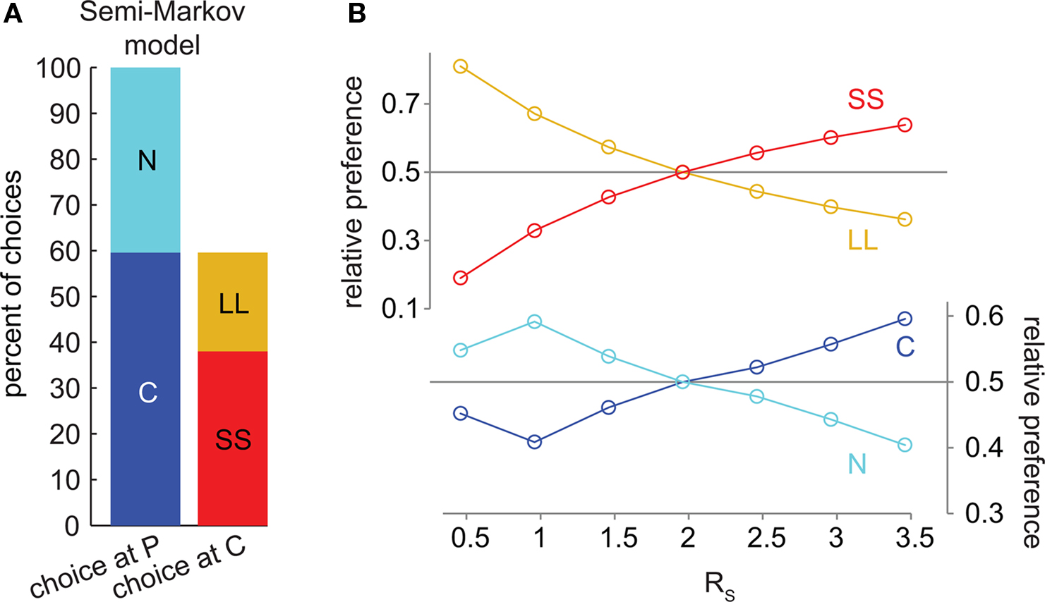
Figure 5. The semi-Markov model of hyperbolic discounting (without distributed discounting) cannot produce precommitment behavior. (A) At the selected parameters, SS was preferred to LL and C was preferred to N. This bar graph represents the same data as (B) at R_S = 3.46. (B) As R_S increased, the preference for C overtook N exactly at the same point as the preference for SS overtook LL, meaning that this model would not precommit to avoid an impulsive choice. Note that in this model, each state has a long temporal extent (and replacing long states with one-step states produces different discounting), so it is not possible to plot intermediate discounted values as in Figures 2C, 3C, and 4C.

Precommitment Depends on Task Parameters

Precommitment is behavior that avoids the opportunity to choose an impulsive option even though that option would be preferred given the choice. In order to understand what kind of situations are most favorable to precommitment behavior, we looked at how precommitment preference can be maximized for a given ratio of preference between SS and LL. We again looked at precommitment over a range of R_S, but this time adjusted D_S concurrently with R_S such that (the discounted value of the SS option) was held constant. We found that a smaller R_S (paired with a correspondingly shorter D_S) was always more favorable to precommitment (Figure 6A). In other words, the model was more likely to precommit when the impulsive choice was smaller and more immediate. Equivalently, a very large, very late LL choice always produced greater precommitment than an equivalently valued but modestly large and late LL choice. (Decreasing R_S is equivalent to increasing R_L, because choice is unaffected by equal scaling of the two reward magnitudes.)

FIGURE 6

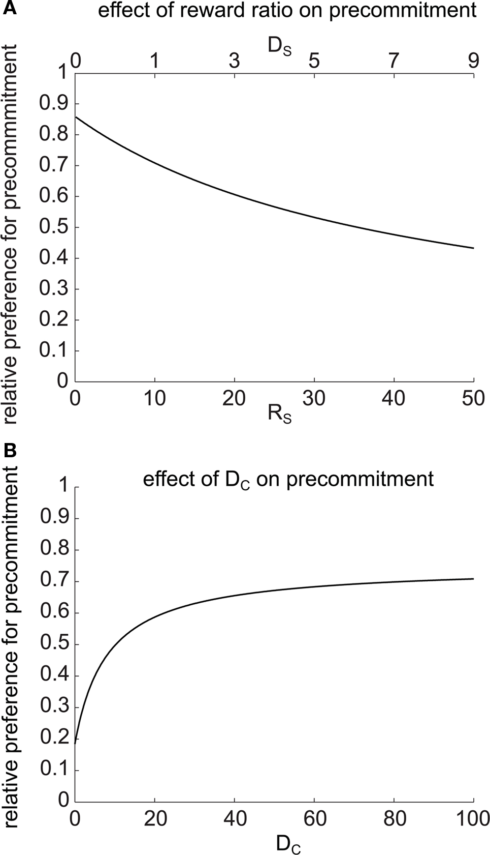
Figure 6. Precommitment depends on task parameters. (A) Precommitment was greater when the reward ratio R_L/R_S was larger. On the x axis, D_S and R_S were simultaneously manipulated so that the SS vs. LL preference was held constant. Despite the constant SS vs. LL preference, the preference for precommitment increased as the size of the small reward decreased. (B) Precommitment increases with the delay (D_C) between commitment and choice. At the selected parameters, LL was preferred 0.196 as much as SS. When there was no delay between commitment and choice, C was preferred over N by the same ratio. As D_C increased, the relative preference for N increased, despite no change in the relative preference for SS vs. LL. This figure was generated with mathematical hyperbolic discounting.

We next investigated the effect of changing the delay D_C on precommitment behavior. Rachlin and Green (1972) observed that precommitment increases as the delay increases between the first and second choices. To look for a similar effect in the model, we plotted the relative preference for N (i.e., ) against a changing D_C (Figure 6B). As D_C increased, we observed an increase in preference for N, asymptotically approaching a constant as D_C → ∞. This matches the result of Rachlin and Green (1972). We found a qualitatively similar effect of varying D_C for any given values of k, D_S, R_S, D_L, and R_L (data not shown).

The delay D_C occurred before the SS vs. LL choice and therefore did not affect the relative preference for these options. This means that although the model held a constant preference for SS over LL as D_C varied, the model switched from strongly preferring not to precommit to strongly preferring to precommit as D_C increased.

Precommitment Depends on Discount Rate

In the model, hyperbolic discounting arises as the average of many exponential discount curves. If the discount rates of the individual exponential functions are spread uniformly over the interval (0,1), then the sum of these functions approaches (as N_μ → ∞) a hyperbolic function with k = 1. Altering the distribution of exponential discount rates to a non-uniform distribution alters the resulting average and can produce hyperbolic functions with any desired value of k (Kurth-Nelson and Redish, 2009).

We took advantage of this to test the behavior of the model at different values of k. We found that the effect of varying k depended on the task parameters. Specifically, the effect of changing k was opposite for different values of D_C (Figure 7A). For small D_C, faster discounting (larger k) led to less precommitment (Figure 7B). But for large D_C, faster discounting led to more precommitment (Figure 7C). As k increased, the relative preference for smaller-sooner over larger-later also increased (not shown). The reason for these opposite results at different values of D_C is that increasing k has two effects. First, it boosts the preference for SS over LL. Second, it makes the D_C interval effectively longer (because k is simply a time dilation factor), so the difference in discounting between D_C + D_S and D_C + D_L is diminished. The first effect dominates when D_C is small, and the second effect dominates when D_C is large.

FIGURE 7

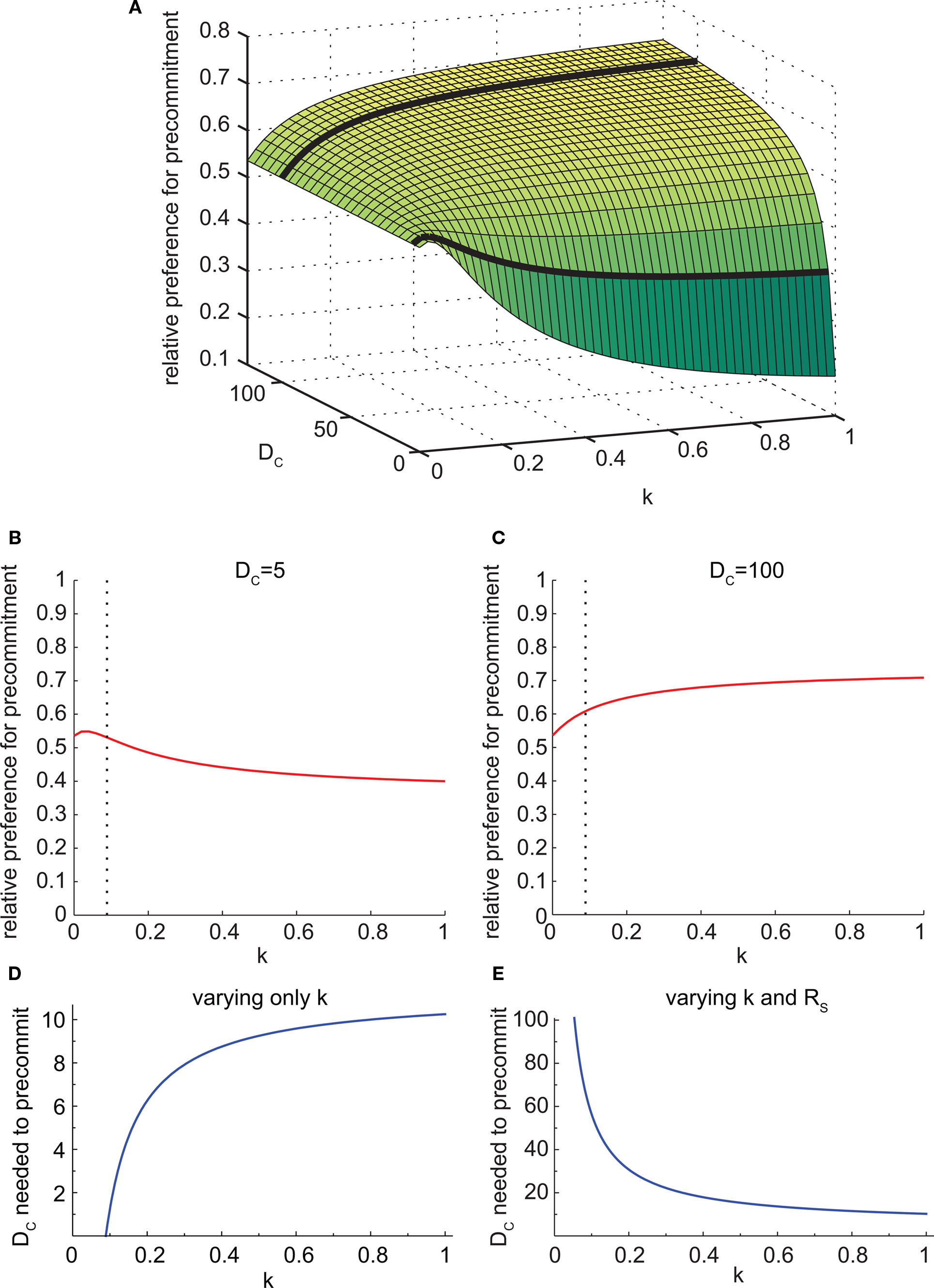
Figure 7. The discounting rate has a complex interaction with precommitment behavior. (A) Precommitment preference plotted against k and D_C. The heavy black lines show the intersection of the planes D_C = 5 and D_C = 100 with this surface, representing the lines in (B) and (C). (B) When D_C was small (D_C = 5), faster discounting yielded less precommitment. The dashed line represents the value of k above which SS was preferred over LL. (C) When D_C was large (D_C = 100), faster discounting yielded greater precommitment. The dashed line represents the value of k above which SS was preferred over LL. (D) As k increased, the amount of D_C required to prefer precommitment also increased. Faster discounting increased the amount of D_C required to produce precommitment. When k was less than 4/45, LL was preferred over SS, so N was preferred over C even when there was no precommitment delay. (E) The SS–LL preference ratio was held constant by adjusting R_S. Under this condition, the amount of D_C required to precommit grew as k increased. In other words, for a given SS–LL preference, agents with slower discounting will require a much longer D_C to achieve precommitment. This figure was generated with mathematical hyperbolic discounting.

As k increased, the amount of delay D_C needed to produce precommitment also increased (Figure 7D). This is because faster discounters have a stronger preference for SS over LL, and more D_C was needed to overcome this preference. However, if k was manipulated while holding the SS vs. LL preference constant (by adjusting the magnitude of R_S), then the opposite effect was seen. For a given degree of preference for SS over LL, faster discounters required less D_C to achieve precommitment (Figure 7E).

Precommitment Depends on Shape of Discount Curve

As described above, the fidelity of the model’s approximation to true hyperbolic discounting depended on the number of μAgents. Because precommitment in the model depended on non-exponential discounting, we investigated how changing the number of μAgents influenced precommitment behavior. With 1000 μAgents, the model produced precommitment that was very similar to the precommitment produced by true hyperbolic discounting. However, we found that reducing the number of μAgents to 100 eliminated precommitment preference under the selected parameters (Figure 8A). The difference between the discount curves with 100 vs. 1000 exponentials was slight (Figure 8B), indicating that precommitment behavior is highly sensitive to the precise shape of the discount curve.

FIGURE 8

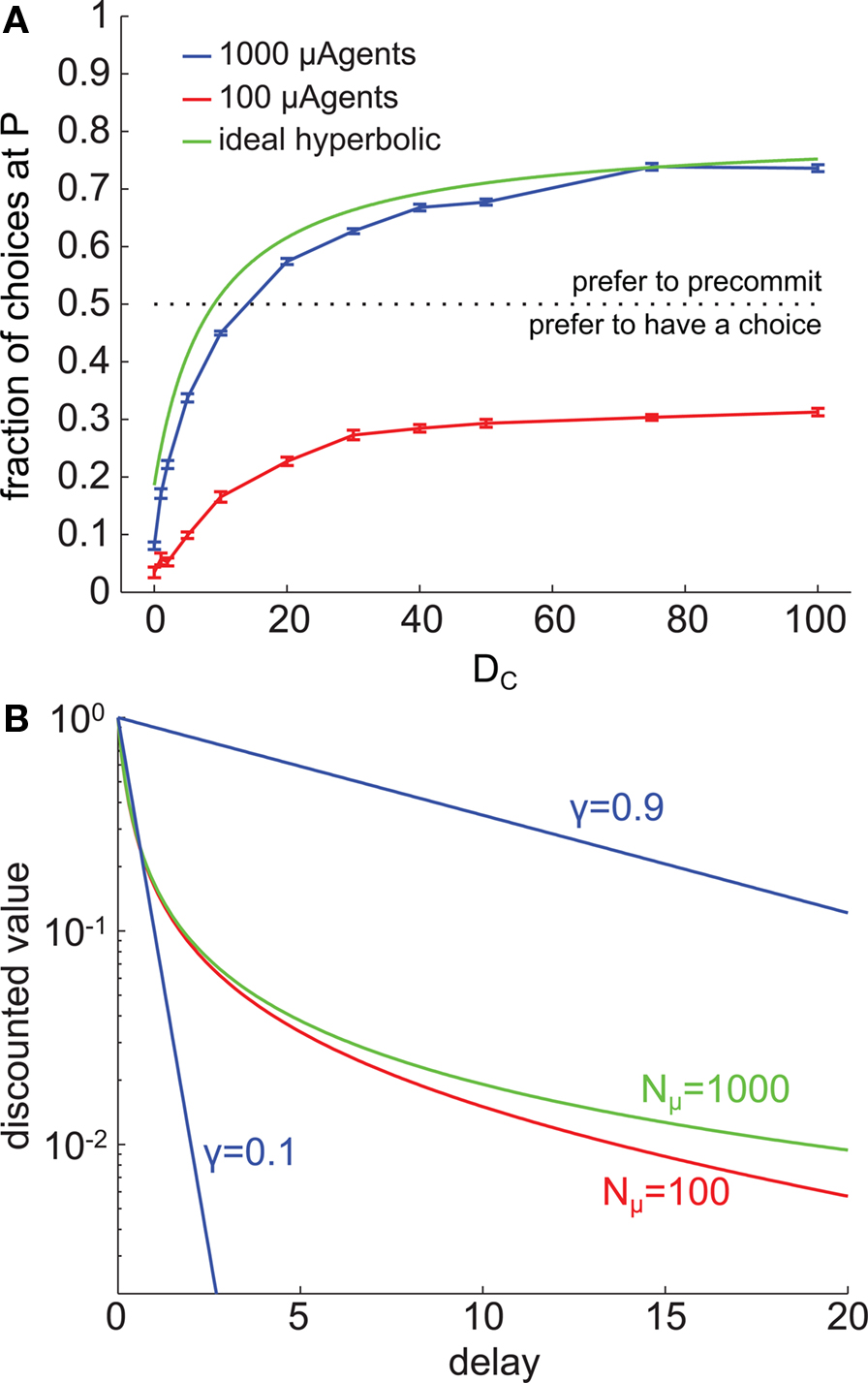
Figure 8. Precommitment is highly dependent on the shape of the discount curve. (A) These graphs plot the average (across 200 trials) number of times each choice was selected at different values of D_C. The blue line shows choices made when N_μ = 1000, and the red line shows choices made when N_μ = 100. (B) The shape of the average discount function depends on the number of μAgents. Red shows the average discounting of 100 μAgents and green shows the average discounting of 1000 μAgents. If a perfect hyperbolic function is plotted on this graph, it overlies the green curve. For reference, exponential discount curves with γ = 0.1 and γ = 0.9 are plotted in blue. The vertical axis is log scale to make visible the separation of the red and green curves. In this figure, k = 5.

To understand why precommitment occurred with 1000 but not with 100 μAgents, we tested the model with 100 μAgents but adjusted the slowest γ from 0.99 to 0.999 (0.999 is the slowest γ when there are 1000 μAgents). This adjustment was sufficient to recover precommitment behavior (data not shown), suggesting that the presence of this very slow discounting component was necessary for precommitment. The γ = 0.999 μAgent had little relative effect on values that are discounted over short delays, because those average values received a significant contribution from other μAgents. But on values discounted over long delays, the γ = 0.999 μAgent had a predominant effect, contributing far more than 1/100th of the average value. The γ = 0.999 μAgent effectively propped up the tail of the average discount curve without having a significant impact on the early part of the curve. This enhanced the degree of preference reversal inherent in the curve, which is the feature essential for precommitment.

Discussion

In this paper, we have presented a reinforcement learning account of precommitment. The advance decision (precommitment) to avoid an impulsive choice is a natural consequence of hyperbolic discounting, because in hyperbolic discounting, preferences reverse as a choice is viewed from a distance. Our model performs hyperbolic discounting by using a set of independent “μAgents” performing exponential discounting in parallel, each at a different rate. This model demonstrates that a reinforcement learning system, implementing hyperbolic discounting, can exhibit precommitment. Precommitment also illustrates the more general problem of non-exponential discounting in complex state-spaces that include choices. To our knowledge, no other reinforcement learning models of hyperbolic discounting function correctly in such state-spaces. It is interesting to note that our model also matches Ainslie’s (1975) prediction for bundled choices. Ainslie observed that even if SS is preferred when a choice is considered in isolation, hyperbolic discounting implies that if the present choice dictates the outcome of several future choices, LL may be preferred. Because our model implements hyperbolic discounting over complex state-spaces, it matches this prediction (data not shown).

In this paper, we have also made quantitative predictions about precommitment behavior, extending the work of Ainslie (1975, 2001). Except for the prediction that subtle changes in the discount curve affect precommitment, all of the predictions here are general consequences of hyperbolic discounting, whether in a model-free or model-based system, and do not depend specifically on the μAgents model. To our knowledge, none of these predictions have been tested behaviorally. These predictions may inform the development of strategies to encourage precommitment behavior in patients with addiction.

Predictions of the Model and Implications for Treating Addiction

Avoiding situations where a drug choice is immediately available may be the most important step in recovery from addiction. In this section, we outline the predictions of our model and discuss the implications for what factors may bias addicts’ decisions toward choosing to avoid such situations.

Pigeons show increased precommitment behavior when the delay (called D_C in this paper) between the first and second choice is increased (Rachlin and Green, 1972). Our model reproduced this result (Figure 6B). This suggests that when designing precommitment interventions, long pre-choice delays are critical. An addict with a bag of heroin in his pocket may not choose to take methadone, but if the choice to take methadone could be presented further in advance, the addict may be willing to precommit. In general, if we can find out when addicts are going to have access to drug choices, we should offer precommitment devices as far in advance from these choices as possible.

Hyperbolic discounting also implies other properties of precommitment behavior. These properties would hold in any model that correctly implements hyperbolic discounting across multiple choices. First, hyperbolic discounting predicts that precommitment will be most differentially reinforced when the smaller-sooner reward is small in magnitude relative to the larger-later reward (Figure 6A). This is true even when the delays are modulated such that the two rewards themselves retain the same preference ratio. Thus a very large, very late reward should be more effective at producing precommitment than a modest but earlier delayed reward. Likewise, precommitment interventions are likely to be more successful when the impulsive choice is more immediate. This is promising for treatment because often the “larger-later” reward is a healthy, productive life, which is very large and very late. This prediction also suggests that precommitment devices may be more useful for drugs that deliver a small reward following a short latency, such as cigarettes.

Second, hyperbolic discounting predicts that precommitment behavior is influenced by discount rate. In situations where D_C is small, a faster discount rate makes the model less likely to precommit (Figure 7B). On the other hand, when D_C is large, a faster discount rate actually makes the model more likely to precommit (Figure 7C). Conversely, this means that individuals with a faster discount rate will see more benefit from lengthening D_C. This result runs counter to the intuition that impulsive, fast discounting individuals would be less likely to commit to long-range strategies. In fact, they are very likely to commit, because when the choice is viewed in advance, the SS and LL discount nearly identically, and the LL has a larger magnitude. In other words, for faster discounters, the hyperbolic curve flattens out faster. For a given degree of preference for SS over LL, faster discounters require less D_C to prefer precommitment (Figure 7E). This implies that measuring an individual’s discount rate could help to determine what intervention strategies will be effective. If an individual is on the cusp of indecision, offering a precommitment device with a short delay may be sufficient for faster discounters, but ineffective for slow discounters. This also suggests the idea of two different addiction phenotypes, one for slow discounters and one for fast discounters. Slow discounters may not respond to the intervention strategies that work for fast discounters.

The μAgents model also makes a prediction that is not made by hyperbolic discounting alone. Subtle changes in the shape of the discount function, independent of overall discount rate, alter the preference for precommitment (Figure 8). This has two implications. First, it is likely that whatever the mechanism of discounting in humans and animals, it is not perfectly hyperbolic. Small fluctuations in the shape of the curve could determine whether an individual is willing to precommit. These differences could occur between individuals, in which case measuring precisely the shape of the discounting curve for an individual could help establish treatment patterns. The fluctuations could also occur within an individual over time (Mobini et al., 2000; Schweighofer et al., 2008), and may help to explain both spontaneous relapse and spontaneous recovery. Second, if humans and animals implement some form of distributed discounting, precommitment could be a very sensitive assay to determine exactly how discounting is being calculated.

Discount curves can be changed by context (Dixon et al., 2006), diet (Schweighofer et al., 2008), pharmacological state (de Wit et al., 2002), availability of working memory capacity (Hinson et al., 2003), and possibly cognitive training (Kendall and Wilcox, 1980; Nelson and Behler, 1989). For example, Schweighofer et al. (2008) showed that increasing dietary tryptophan slows discounting, and specifically increases task-related activation of parts of the striatum associated with slow discounting (Tanaka et al., 2007). Such manipulations could potentially have a large impact on whether people decide to engage in precommitment strategies.

Neurobiology of Precommitment

Reinforcement learning models have been used to describe the learning processes embodied in the basal ganglia (Doya, 1999). During learning tasks, midbrain dopamine neurons fire in a pattern that closely matches the δ signal of temporal difference reinforcement learning (Ljungberg et al., 1992; Montague et al., 1996; Hollerman and Schultz, 1998). Both functional imaging and electrophysiological recording suggest that cached values are represented in striatum (Samejima et al., 2005; Tobler et al., 2007). The hypothesis that these brain structures implement reinforcement learning has helped to link a theoretical understanding of behavior with neurophysiological experiments.

If certain brain structures implement reinforcement learning, then reinforcement learning models may also be able to make predictions about the neurophysiology of precommitment. For example, our model implies that if precommitment is the preferred strategy, then selecting the choice option should produce a pause in dopamine firing (at the transition from P to C, the average δ is , which is negative because .

There is also some evidence that the brain may implement distributed discounting. A sum of exponentials may in some cases be a statistically better fit to the time courses of human forgetting (Rubin and Wenzel, 1996; Rubin et al., 1999), suggesting the possibility of a distributed learning and memory process. During delay discounting tasks, there is a distribution across the striatum of areas correlated with different discount rates (Tanaka et al., 2004), consistent with the theory of a distributed set of agents exponentially discounting in parallel. For a more complete discussion of the evidence for distributed discounting, see Kurth-Nelson and Redish (2009).

Some have argued that the brain implements a decision-making system in which each reward is assigned a single hyperbolically discounted subjective value (Kable and Glimcher, 2009), as suggested by fMRI correlates of hyperbolically discounted subjective value (Kable and Glimcher, 2007). However, fMRI is spatially and temporally averaged, which could blur an underlying distribution of exponentials to look like a hyperbolic representation. Even if the fMRI data do reflect an underlying hyperbolic representation, this does not disprove the existence of multiple exponentials elsewhere in the brain. A distribution of exponentials would need to be averaged before taking an action, producing a hyperbolic representation downstream.

In order to precommit, hyperbolic discounting must function across multiple state transitions, which in general is not possible in a non-distributed system that estimates values using only local information. If the brain represents single hyperbolically discounted values at each state, then the decision-making system must use some type of non-local information, such as multiple variables to track the time until each possible reward, or a look-ahead system to anticipate future rewards.

To our knowledge, precommitment of the form described here has not been empirically studied in humans. If precommitment is a product of reinforcement learning, implemented in the basal ganglia, then interfering with these brain structures should prevent precommitment. For example, Parkinson’s patients would be impaired in learning precommitment strategies. On the other hand, brain structures such as frontal cortex that are not necessary for basic operant conditioning would not be necessary for precommitment.

Multiple Systems and Cognitive Precommitment

In this paper we have presented a model of precommitment arising from hyperbolic discounting in an automated (habitual, model-free) learning system, using cached values to decide on actions without planning or cognitive involvement. An alternative possibility is that precommitment may be produced by a cognitive (look-ahead, model-based) system. The role for an interaction between automated and cognitive systems has been discussed extensively, especially in the context of impulsive choice and addiction (Tiffany, 1990; Bickel et al., 2007; Redish et al., 2008; Gläscher et al., 2010). The cognitive system might recognize that the automated system will make a suboptimal choice and precommit to effectively override the automated system (“If I go to the bar, I will drink. Therefore I will not go to the bar.”) (Ainslie, 2001; Bernheim and Rangel, 2004; Isoda and Hikosaka, 2007; Johnson et al., 2007; Redish et al., 2008). Rats appear to project themselves mentally into the future when making a difficult decision (Johnson and Redish, 2007). In humans, vividly imagining a delayed outcome slows the discounting to that outcome (Peters and Büchel, 2010). Constructing a cognitive representation of the future may allow an individual to carefully weigh the possible outcomes, even when those outcomes have never been experienced. The cognitive resources needed for this deliberation may be depleted by placing demands on working memory (Hinson et al., 2003) or self-control (Vohs et al., 2008).

Both automated and cognitive systems are likely to play a role in precommitment. To begin to identify the role of each system, we should look at the empirically distinguishable properties of precommitment produced by each system. First, if precommitment comes from an automated system, it should not be sensitive to attention or to cognitive load. A cognitive mechanism of precommitment would likely be sensitive to attention and cognitive load. Second, the automated system hypothesis predicts that precommitment would require learning; an individual must be repeatedly exposed to the outcomes and would not choose to precommit in novel situations. A cognitive model would predict that precommitment could occur in novel situations. Third, the automated model predicts that fast discounters are more likely than slow discounters to commit to long-range precommitment strategies. It seems likely that a cognitive model would predict the opposite. Fourth, the two hypotheses predict the involvement of different brain structures in precommitment. The automated hypothesis predicts that learning requires basal ganglia structures such as striatum and ventral tegmental area, while the cognitive hypothesis predicts the involvement of cortex and hippocampus. Testing these predictions should provide clues about the possible role of cognitive systems in precommitment.

Conflict of Interest Statement

The authors declare that the research was conducted in the absence of any commercial or financial relationships that could be construed as a potential conflict of interest.

Acknowledgment

This work was funded by National Institutes of Health Grant R01 DA024080.

Footnotes

1. ^To be precise, this is the economic notion of impulsivity; impulsivity can also refer to making a decision without waiting for sufficient information, inability to stop a prepotent action, and other related phenomena. But these other phenomena entail different mechanisms and are dissociable from delay discounting (Evenden, 1999; Reynolds et al., 2006).
2. ^Note that in this paper, a state contains a delay that is preceded by value of that state and followed by the reward (if any) of the state; this sequence is slightly different from Kurth-Nelson and Redish (2009), where reward comes at the “beginning” of the state. This difference has no effect on the behavior of the model.
3. ^This is because the last C state transitioned to both the first SS state and the first LL state. In temporal difference learning, the value of a state with multiple transitions going out will converge to a weighted average of the discounted next states’ value plus reward. The average is weighted by the relative frequency of making each transition, which in this case is determined by the agent’s choice. Thus, the model is “sophisticated” (O’Donoghue and Rabin, 1999): the knowledge that it will choose SS is encoded in the value of the C state.

References

Ainslie, G. (1974). Impulse control in pigeons. J. Exp. Anal. Behav. 21, 485–489.

Pubmed Abstract | Pubmed Full Text | CrossRef Full Text

Ainslie, G. (1975). Specious reward: a behavioral theory of impulsiveness and impulse control. Psychol. Bull. 82, 463–496.

Pubmed Abstract | Pubmed Full Text | CrossRef Full Text

Ainslie, G. (1992). Picoeconomics. Cambridge: Cambridge University Press.

Ainslie, G. (2001). Breakdown of Will. Cambridge: Cambridge University Press.

Alexander, W. H., and Brown, J. W. (2010). Hyperbolically discounted temporal difference learning. Neural. Comput. 22, 1511–1527.

Pubmed Abstract | Pubmed Full Text | CrossRef Full Text

Bellman, R. (1958). On a routing problem. Q. J. Appl. Math. 16, 87–90.

Bernheim, B. D., and Rangel, A. (2004). Addiction and cue-triggered decision processes. Am. Econ. Rev. 94, 1558–1590.

CrossRef Full Text

Bickel, W. K., Miller, M. L., Yi, R., Kowal, B. P., Lindquist, D. M., and Pitcock, J. A. (2007). Behavioral and neuroeconomics of drug addiction: competing neural systems and temporal discounting processes. Drug Alcohol Depend. 90, S85–S91.

Pubmed Abstract | Pubmed Full Text | CrossRef Full Text

Bickel, W. K., Odum, A. L., and Madden, G. J. (1999). Impulsivity and cigarette smoking: delay discounting in current, never, and ex-smokers. Psychopharmacology (Berl.) 146, 447–454.

Pubmed Abstract | Pubmed Full Text | CrossRef Full Text

Coffey, S. F., Gudleski, G. D., Saladin, M. E., and Brady, K. T. (2003). Impulsivity and rapid discounting of delayed hypothetical rewards in cocaine-dependent individuals. Exp. Clin. Psychopharmacol. 11, 18–25.

Pubmed Abstract | Pubmed Full Text | CrossRef Full Text

Daw, N. D. (2003). Reinforcement Learning Models of the Dopamine System and Their Behavioral Implications. Ph.D. thesis, Carnegie Mellon University, Pittsburgh.

Daw, N. D., and Touretzky, D. S. (2000). Behavioral considerations suggest an average reward TD model of the dopamine system. Neurocomputing 32–33, 679–684.

CrossRef Full Text

de Wit, H., Enggasser, J. L., and Richards, J. B. (2002). Acute administration of d-amphetamine decreases impulsivity in healthy volunteers. Neuropsychopharmacology 27, 813–825.

Pubmed Abstract | Pubmed Full Text | CrossRef Full Text

Dezfouli, A., Piray, P., Keramati, M. M., Ekhtiari, H., Lucas, C., and Mokri, A. (2009). Aneurocomputational model for cocaine addiction. Neural Comput. 21, 2869–2893.

Pubmed Abstract | Pubmed Full Text | CrossRef Full Text

Dixon, M. R., Jacobs, E. A., and Sanders, S. (2006). Contextual control of delay discounting by pathological gamblers. J. Appl. Behav. Anal. 39, 413–422.

Pubmed Abstract | Pubmed Full Text | CrossRef Full Text

Dom, G., D’haene, P., Hulstijn, W., and Sabbe, B. (2006). Impulsivity in abstinent early- and late-onset alcoholics: differences in self-report measures and a discounting task. Addiction 101, 50–59.

Pubmed Abstract | Pubmed Full Text | CrossRef Full Text

Doya, K. (1999). What are the computations of the cerebellum, the basal ganglia, and the cerebral cortex? Neural Netw. 12, 961–974.

Pubmed Abstract | Pubmed Full Text | CrossRef Full Text

Dripps, D. A. (1993). Precommitment, prohibition, and the problem of dissent. J. Legal Stud. 22, 255–263.

CrossRef Full Text

Evenden, J. L. (1999). Varieties of impulsivity. Psychopharmacology 146, 348–361.

Pubmed Abstract | Pubmed Full Text | CrossRef Full Text

Fishburn, P. C., and Rubinstein, A. (1982). Time preference. Int. Econ. Rev. 23, 677–694.

CrossRef Full Text

Frederick, S., Loewenstein, G., and O’Donoghue, T. (2002). Time discounting and time preference: a critical review. J. Econ. Lit. 40, 351–401.

CrossRef Full Text

Gläscher, J., Daw, N., Dayan, P., and O’Doherty, J. P. (2010). States versus rewards: dissociable neural prediction error signals underlying model-based and model-free reinforcement learning. Neuron 66, 585–595.

CrossRef Full Text

Hinson, J. M., Jameson, T. L., and Whitney, P. (2003). Impulsive decision making and working memory. J. Exp. Psychol. Learn. Mem. Cogn. 29, 298–306.

Pubmed Abstract | Pubmed Full Text | CrossRef Full Text

Hollerman, J. R., and Schultz, W. (1998). Dopamine neurons report an error in the temporal prediction of reward during learning. Nat. Neurosci. 1, 304–309.

Pubmed Abstract | Pubmed Full Text | CrossRef Full Text

Isoda, M., and Hikosaka, O. (2007). Switching from automatic to controlled action by monkey medial frontal cortex. Nat. Neurosci. 10, 240–248.

Pubmed Abstract | Pubmed Full Text | CrossRef Full Text

Johnson, A., and Redish, A. D. (2007). Neural ensembles in CA3 transiently encode paths forward of the animal at a decision point. J. Neurosci. 27, 12176–12189.

Pubmed Abstract | Pubmed Full Text | CrossRef Full Text

Johnson, A., van der Meer, M. A., and Redish, A. D. (2007). Integrating hippocampus and striatum in decision-making. Curr. Opin. Neurobiol. 17, 692–697.

Pubmed Abstract | Pubmed Full Text | CrossRef Full Text

Kable, J. W., and Glimcher, P. W. (2007). The neural correlates of subjective value during intertemporal choice. Nat. Neurosci. 10, 1625–1633.

Pubmed Abstract | Pubmed Full Text | CrossRef Full Text

Kable, J. W., and Glimcher, P. W. (2009). The neurobiology of decision: consensus and controversy. Neuron 63, 733–745.

Pubmed Abstract | Pubmed Full Text | CrossRef Full Text

Kendall, P. C., and Wilcox, L. E. (1980). Cognitive-behavioral treatment for impulsivity: concrete versus conceptual training in non-self-controlled problem children. J. Consult. Clin. Psychol. 48, 80–91.

Pubmed Abstract | Pubmed Full Text | CrossRef Full Text

Koopmans, T. C. (1960). Stationary ordinal utility and impatience. Econometrica 28, 287–309.

CrossRef Full Text

Kurth-Nelson, Z., and Redish, A. D. (2009). Temporal-difference reinforcement learning with distributed representations. PLoS One 4:e7362. doi:10.1371/journal.pone.0007362.

Pubmed Abstract | Pubmed Full Text | CrossRef Full Text

Ljungberg, T., Apicella, P., and Schultz, W. (1992). Responses of monkey dopamine neurons during learning of behavioral reactions. J. Neurophysiol. 67, 145–163.

Pubmed Abstract | Pubmed Full Text

Madden, G. J., and Bickel, W. K. (2010). Impulsivity: The Behavioral and Neurological Science of Discounting. Washington, DC: American Psychological Association.

Madden, G. J., Petry, N. M., Badger, G. J., and Bickford, W. K. (1997). Impulsive and self-control choices in opioid-dependent patients and non-drug-using control patients: drug and monetary rewards. Exp. Clin. Psychopharmacol. 5, 256–262.

Pubmed Abstract | Pubmed Full Text | CrossRef Full Text

Mazur, J. (1987). “An adjusting procedure for studying delayed reinforcement,” in Quantitative Analysis of Behavior: Vol. 5. The Effect of Delay and of Intervening Events on Reinforcement Value, eds M. L. Commons, J. F. Mazur, J. A. Nevin, and H. Rachlin (Hillsdale, NJ: Erlbaum), 55–73.

Mobini, S., Chiang, T. J., Al-Ruwaitea, A. S., Ho, M. Y., Bradshaw, C. M., and Szabadi, E. (2000). Effect of central 5-hydroxytryptamine depletion on inter-temporal choice: a quantitative analysis. Psychopharmacology 149, 313–318.

Pubmed Abstract | Pubmed Full Text | CrossRef Full Text

Montague, P. R., Dayan, P., and Sejnowski, T. J. (1996). A framework for mesencephalic dopamine systems based on predictive Hebbian learning. J. Neurosci. 16, 1936–1947.

Pubmed Abstract | Pubmed Full Text

Nelson, W. M., and Behler, J. J. (1989). Cognitive impulsivity training: the effects of peer teaching. J. Behav. Ther. Exp. Psychiatry 20, 303–309.

Pubmed Abstract | Pubmed Full Text | CrossRef Full Text

O’Donoghue, T., and Rabin, M. (1999). Doing it now or later. Am. Econ. Rev. 89, 103–124.

CrossRef Full Text

Peters, J., and Büchel, C. (2010). Episodic future thinking reduces reward delay discounting through an enhancement of prefrontal-mediotemporal interactions. Neuron 66, 138–148.

Pubmed Abstract | Pubmed Full Text | CrossRef Full Text

Rachlin, H., and Green, L. (1972). Commitment, choice, and self-control. J. Exp. Anal. Behav. 17, 15–22.

Pubmed Abstract | Pubmed Full Text | CrossRef Full Text

Redish, A. D., Jensen, S., and Johnson, A. (2008). A unified framework for addiction: vulnerabilities in the decision process. Behav. Brain Sci. 31, 415–437.

Pubmed Abstract | Pubmed Full Text | CrossRef Full Text

Reynolds, B., Ortengren, A., Richards, J. B., and Wit, H. D. (2006). Dimensions of impulsive behavior: Personality and behavioral measures. Pers. Individ. Dif. 40, 305–315.

CrossRef Full Text

Rubin, D. C., Hinton, S., and Wenzel, A. (1999). The precise time course of retention. J. Exp. Psychol. Learn. Mem. Cogn. 25, 1161–1176.

CrossRef Full Text

Rubin, D. C., and Wenzel, A. E. (1996). One hundred years of forgetting: a quantitative description of retention. Psychol. Rev. 103, 734–760.

CrossRef Full Text

Samejima, K., Ueda, Y., Doya, K., and Kimura, M. (2005). Representation of action-specific reward values in the striatum. Science 310, 1337–1340.

Pubmed Abstract | Pubmed Full Text | CrossRef Full Text

Samuelson, P. A. (1937). A note on measurement of utility. Rev. Econ. Stud. 4, 155–161.

CrossRef Full Text

Schweighofer, N., Bertin, M., Shishida, K., Okamoto, Y., Tanaka, S. C., Yamawaki, S., and Doya, K. (2008). Low-serotonin levels increase delayed reward discounting in humans. J. Neurosci. 28, 4528–4532.

Pubmed Abstract | Pubmed Full Text | CrossRef Full Text

Sozou, P. D. (1998). On hyperbolic discounting and uncertain hazard rates. Proc. Biol. Sci. 265, 2015–2020.

CrossRef Full Text

Strotz, R. H. (1955). Myopia and inconsistency in dynamic utility maximization. Rev. Econ. Stud. 23, 165–180.

CrossRef Full Text

Sutton, R. S., and Barto, A. G. (1998). Reinforcement Learning: An Introduction. Cambridge, MA: MIT Press.

Tanaka, S. C., Doya, K., Okada, G., Ueda, K., Okamoto, Y., and Yamawaki, S. (2004). Prediction of immediate and future rewards differentially recruits cortico-basal ganglia loops. Nat. Neurosci. 7, 887–893.

Pubmed Abstract | Pubmed Full Text | CrossRef Full Text

Tanaka, S. C., Schweighofer, N., Asahi, S., Shishida, K., Okamoto, Y., Yamawaki, S., and Doya, K. (2007). Serotonin differentially regulates short- and long-term prediction of rewards in the ventral and dorsal striatum. PLoS One 2:e1333. doi: 10.1371/journal.pone.0001333.

Pubmed Abstract | Pubmed Full Text | CrossRef Full Text

Tiffany, S. T. (1990). A cognitive model of drug urges and drug-use behavior: role of automatic and nonautomatic processes. Psychol. Rev. 97, 147–168.

Pubmed Abstract | Pubmed Full Text | CrossRef Full Text

Tobler, P. N., O’Doherty, J. P., Dolan, R. J., and Schultz, W. (2007). Reward value coding distinct from risk attitude-related uncertainty coding in human reward systems. J. Neurophysiol. 97, 1621–1632.

Pubmed Abstract | Pubmed Full Text | CrossRef Full Text

Tsitsiklis, J. N., and Van Roy, B. (1999). Average cost temporal-difference learning. Automatica 35, 1799–1808.

CrossRef Full Text

Vohs, K. D., Baumeister, R. F., Schmeichel, B. J., Twenge, J. M., Nelson, N. M., and Tice, D. M. (2008). Making choices impairs subsequent self-control: a limited-resource account of decision making, self-regulation, and active initiative. J. Pers. Soc. Psychol. 94, 883–898.

Pubmed Abstract | Pubmed Full Text | CrossRef Full Text