Associative Learning Through Acquired Salience

Introduction

In nature, visual stimuli are organized in complex combinations. Animals must focus their visual system on salient objects from visual scenes to extract relevant information for guiding their behavior. The physical properties of the stimuli (v.gr. their structure or intensity) contribute to establishing how salient or conspicuous they are (Itti and Koch, 2001; Pearce and Bouton, 2001). Such effective salience specifies the relative capacity of a stimulus to stand out among other items in the visual scene. Consequently, salient stimuli attract attention and increase the rate of learning about them as well as other similar visual objects (Rescorla and Wagner, 1972; Mackintosh, 1975; Le Pelley, 2004; Treviño et al., 2013). From both behavioral and neurobiological perspectives, salience is a fundamental stimulus-specific learning rate parameter.

Associative learning theories propose that the increments of associative strength decrease linearly as a function of that value (Bush and Mosteller, 1951). Many models propose that the rate of conditioning also depends on stimulus salience, but they generally represent it as a fixed quantity that depends on the physical attributes of the stimulus (Rescorla and Wagner, 1972). Thus, from this point of view, the contribution of discriminative stimuli to learning would be fixed and determined, exclusively, by their effective salience. There is a body of literature, however, that reveals that this notion is incomplete. For example, learning about an item depends on the amount of visual attention that is paid to it (McFarland, 1971; Mackintosh, 1975; Ahissar and Hochstein, 1993; Jiang and Chun, 2001; Baker et al., 2004; Harris, 2006; Griffiths and Mitchell, 2008; Gutnisky, 2009; Roelfsema et al., 2010) and, also, pre-exposure to stimuli uncorrelated with reinforcement reduces their associability (Lubow and Moore, 1959). Thus, an interesting possibility would be that discrimination learning also involves dynamic changes in stimulus salience. Salience changes could be related to processes such as motivation, attention, and arousal (Mackintosh, 1975; Koch and Ullman, 1985; Desimone and Duncan, 1995; Kustov and Robinson, 1996; Reynolds et al., 2000). Indeed, some theories of selective attention propose that the salience of a stimulus is not only a fixed consequence of its effective salience, but it also varies with the subject's experience with it and other stimuli (i.e., acquired salience). Esber and Haselgrove (2011) proposed that the net salience of a stimulus can be represented by the sum of effective plus acquired components. From this perspective, the total salience would initially depend on the physical properties of the stimulus, but it would then also vary with experience affecting the way subjects direct their attention toward sensory stimuli (Mackintosh, 1975; Pearce and Hall, 1980; Le Pelley, 2004; Esber and Haselgrove, 2011). There are two main possibilities about how stimulus salience could evolve with learning. One option is that salience would increase if the stimulus “predicts reinforcement more accurately than other stimuli present in the situation” but it would decrease “if it predicts reinforcement less accurately” (Mackintosh, 1975). Alternatively, training stimuli could lose salience as they become better predictors of a consequence (Pearce and Hall, 1980).

We have explored and characterized recently some of the visual learning capacities of adult mice. We trained freely moving animals to learn to discriminate between one conditioned (CS⁺) and multiple non-conditioned (${\text{CS}}_i^{-}$) visual stimuli (i.e., images), which offered different degrees of structural similarity (SSIM) with respect to the CS⁺ Wang et al., 2004; Treviño et al., 2013. We've found that the sign and slope of the SSIM gradients led to markedly different learning curves. More precisely, training with negative similarity gradients led to a faster learning rate and a higher (but less precise) average choice performance than with positive gradients (Treviño et al., 2013). Yet, although we made a detailed characterization of both discrete and continuous behavioral measures during learning (Treviño et al., 2013), we didn't explore whether and how the empirical learning curves could be described from the perspective of associative learning theories. Motivated by this question, we here tested a series of mathematical models aiming to predict the empirical learning curves from the mice trained with varying stimulus similarity (Treviño et al., 2013). We adapted a basic differential equation for associative learning coupled to an operator that defined stimulus salience in various relevant ways. Notably, from the set of tested models, we found that the best predictor was one in which we represented the net salience as the sum of effective plus acquired components, as previously suggested (Esber and Haselgrove, 2011). Thus, our analytic results strongly support the idea that the net stimulus salience can indeed vary as a function of the associative history of discriminative stimuli (Mackintosh, 1975; Pearce and Hall, 1980; Esber and Haselgrove, 2011; Treviño et al., 2013). One implication of this interpretation is that learning about discriminative stimuli depends on the specific effective salience trajectory used to learn about them. We thus propose that, at any given time, the external (effective) and internal (acquired) salience elements determine which predictive value will be assigned to conditioned stimuli (Treviño et al., 2011). Understanding how exactly the brain processes salience is a fundamental step to advance current associative learning theories. Verifiable predictive models could become crucial to understanding aberrant salience acquisition in stressful situations and pathological states like schizophrenia, obsessive-compulsive disorder, and addiction.

Materials and Methods

Animals

We trained behaviorally naïve wild-type male mice (C57BL/6, n = 88, P40-50, Charles River) in a dichotomic visual discrimination task (Figure 1A). Mice were housed individually under a 12/12 h light/dark cycle with free access to food and water. Groups of 4–6 mice were trained during the light phase, 5 days a week. All animal experiments were carried out following the animal welfare guidelines of the Max Planck Society (G-171/10) and the Universidad de Guadalajara (SAGARPA, NOM-062-ZOO-1999), in accordance with the NIH's Guide for the Care and Use of Laboratory Animals. The experimental protocol was approved by the ethics comitee of the Instituto de Neurociencias, Universidad de Guadalajara, Mexico.

FIGURE 1

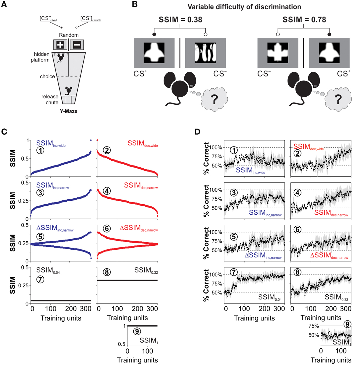
Figure 1. Training paradigms and visual discrimination learning with heterogeneous stimulus similarity. (A) Drawing of the visual discrimination task where two monitors are facing the ends of the arms of a Y-watermaze. They simultaneously display the conditioned (CS⁺) and non-reinforced (CS⁻) equiluminant stimuli (100% contrast). A submerged transparent platform below the CS⁺ serves as the unconditioned stimulus (US). The position of both the CS⁺ and the platform varies randomly on every trial. We placed the mice inside a release chute, and they learned to swim toward the CS⁺ because of the transparent platform positioned below it. (B) Sample CS⁺ stimulus with different CS⁻ stimuli during training trials. The difficulty of the discrimination task depends on the degree of structural similarity (SSIM) between images, indicated on the top. (C) CS⁻ stimuli can be arranged by increasing (blue dots), decreasing (red dots), or constant (black lines) similarity with respect to the CS⁺. (D) Corresponding empirical learning curves for the nine groups of mice trained with the corresponding SSIM programs.

Visual Discrimination Training

We trained the mice using a forced choice, swimming discrimination task in which the mice controlled their decision time autonomously (Treviño et al., 2013). We illustrate a schematic view of the visual swimming task in Figure 1A. In this task, the animals learned to associate that swimming toward a conditioned stimulus (CS⁺) and reaching a transparent submerged platform was rewarded with escape from water, whereas swimming toward a non-conditioned stimulus (CS⁻) was not. For every trial, we displayed the CS⁺ in a different arm of the pool according to a Gellerman-like schedule (Treviño et al., 2011; Herrera and Trevino, 2015). Choices were considered as made, once the animals crossed an imaginary line that outlined a decision area with visual access to both CS⁺ and CS⁻ images (Treviño et al., 2012). The animals were allowed to escape from water 30 s after reaching the submerged platform. We repeated the error trials until the animal made a correct choice (max. five error repetitions). These sets of swims, ranging from 1 to 6, constituted a “training unit,” and they involved the same pair of CS⁺/${\text{CS}}_{\text{i}}^{-}$ images (Figure 1B). The water temperature (21 ± 1°C) and room illumination were kept constant throughout the experiments, and the pool was wiped down daily with ~70% ethanol. A detailed description of other crucial elements of the task have been published previously (Treviño et al., 2013; Treviño, 2014).

To create the training stimuli, we downloaded >1000 pictures from the internet and digitally transformed and scaled them to produce black-and-white, equiluminant (~85 lux) images with different irregularities in shape (Treviño et al., 2013). The resulting images where white shapes on a black background, or vice versa (i.e., the shape was the only relevant “feature”). We further standardized these images by using a symmetric Gaussian low-pass filter (60 pixel size, 30 pixel standard deviation; ~0.30 cycles per degree [c/d]) to remove all the structural components that surpassed a mouse's visual acuity of ~0.48 c/d (Treviño et al., 2012). We illustrate examples of the resulting stimuli in Figure 1B. We next used the structural similarity index (Wang et al., 2004; Treviño et al., 2013; SSIM) to compare the similarity across all combinations of image pairs (Figure 1B), and selected an eccentric CS⁺ that had one of the highest standard deviations of SSIM values against the rest of the CS⁻ images (Treviño et al., 2013).

We next sorted selected CS⁻ with increasing (blue dots) and decreasing (red dots) SSIM values relative to the CS⁺ (Figure 1C); this constituted the stimulus timeline for visual discrimination training. We also created training programs with increasing and decreasing inter-training unit gradients of CS⁺/${\text{CS}}_{\text{i}}^{-}$ similarity (ΔSSIM). With these oscillating SSIM gradients, we investigated how variations in discrimination difficulty, imposed at the beginning or at the end of training influenced learning. Altogether, we formed nine groups of mice and trained them to discriminate images with either varying (Groups 1–6) or fixed (Groups 7–9) SSIM (Table 1).

TABLE 1

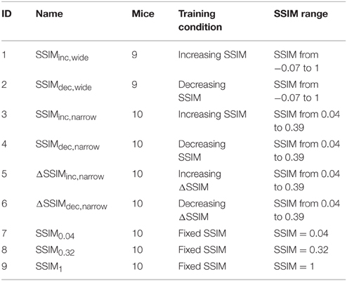
Table 1. Groups of mice trained with varying or fixed stimulus similarity conditions.

The panels in Figures 1C,D are labeled with encircled numbers according to the “IDs” of the groups used in this table. We calculated the average probability of making correct choices (%correct ± %S.E.M) for each trial, and extracted the learning curves of the different groups by using a moving average filter (span = 30 trials, degree = 1; Figure 1D). The data in Figure 1 were published previously (Treviño et al., 2013) and constitute the empirical reference for the mathematical analyses that we developed throughout this work.

Model Fit and Parameter Estimation

To predict the visual discrimination learning curves, we adapted a basic linear operator model of associative learning (Bush and Mosteller, 1951; Rescorla and Wagner, 1972). The model included a minimum salience threshold for learning, as follows:

$\begin{array}{cc}\frac{dV\left(t\right)}{dt}=\{\begin{array}{cc}\alpha \left(t\right)\beta \left[\lambda \left(\alpha \right)-V\left(t\right)\right]& \text{for}\alpha \left(t\right)\ge {\alpha }_{min}\\ -k_{1}V\left(t\right)& \text{for}\alpha \left(t\right)<{\alpha }_{min}\&V\left(t\right)\ge V_{\text{min}}\\ 0& \text{for}\alpha \left(t\right)<{\alpha }_{min}\&V\left(t\right)<V_{min}\end{array}& (1)\end{array}$

where V(t) is the cumulative amount of learning (i.e., the strength of the [CS⁺/${\text{CS}}_{\text{i}}^{-}$]-unconditioned stimulus association); α(t) is the net stimulus salience (related to the CS⁺/${\text{CS}}_{\text{i}}^{-}$ SSIM, see below); β corresponds to the US salience (0 < β < 1; associated with the intensity of the US), and λ(α) is the asymptote of learning (i.e., maximum retention level). The core model for the net salience during training was represented as the sum of effective (ϕ) plus acquired (ε) salience components (Esber and Haselgrove, 2011):

$\begin{array}{ll}\alpha (t)=\varphi (\text{SSIM})+\epsilon (t)& (2)\end{array}$

We defined ϕ and ε as either linear or a non-linear functions of stimulus similarity (SSIM) and the associative strength [V(t)], respectively. We tested for the following salience formulations:

$\begin{array}{l}ModelNr.TotalsalienceEffective+Acquired\\ salience(\varphi )salience(\epsilon (t))\\ Model1(\text{Equation}\text{3}):\alpha \left(t\right)=c_1\\ Model2(\text{Equation}\text{4}):\alpha \left(t\right)=c_1\left(1-SSIM\right)\\ Model3(\text{Equation}\text{5}):\alpha \left(t\right)=c_1{\left(1-SSIM\right)}^{n_1}\\ Model4(\text{Equation}\text{6}):\alpha \left(t\right)=c_1{\left(1-SSIM\right)}^{n_1}+c_{2}V{\left(t\right)}^{n_2}\\ Model5(\text{Equation}\text{7}):\alpha \left(t\right)=c_1{\left(1-SSIM\right)}^{n_1}+c_2{\left({\lambda }_{max}-V\left(t\right)\right)}^{n_2}\\ Model6(\text{Equation}\text{8}):\alpha \left(t\right)=c_1{\left(1-SSIM\right)}^{n_1}+c_2{\left(\left|{\lambda }_{max}-V\left(t\right)\right|\right)}^{n_2}\end{array}$

where c₁, c₂, n₁, and n₂ are constants. Also, we defined λ as a sliding logistic function of the net salience, because we assumed that the quality of sensory representation would degrade gradually as salience reached α_min, compromising discrimination and learning (Treviño et al., 2011):

$\begin{array}{ll}\lambda \left(\alpha \right)=\frac{{\lambda }_{max}}{1+e^{-s\left(\alpha \left(t\right)-{\alpha }_{min}\right)}}& (9)\end{array}$

where s corresponds to the steepness of the sigmoid and α(t) is the net salience of the stimulus. With this core model, we assumed that maximum discrimination performance drops toward zero when α ≤ α_min, but tends toward λ_max for high α values and when k₂ → ∞ (i.e., λ(α) → λ_max) (Rescorla and Wagner, 1972). Also, we assumed that the effective salience of a given stimulus equals that of any other stimulus multiplied by their similarity [ϕ_i(t) = ϕ_j(t)*SSIM_{i, j}] (Mackintosh, 1975; Shepard, 1987; Pearce, 1994; Treviño et al., 2011).

To solve how the associative learning model would fit the experimental learning curves from the mice, we implemented nonlinear programming routines using standard optimization tools from MATLAB (The MathWorks, Inc., USA). With this approach, we aimed finding the best model parameters that produced learning curves that mimicked the empirical correct choice records from the trained mice. Thus, we employed the 2nd order Runge-Kutta method to solve Equation (1) at discrete intervals. Next, to find the model parameters that minimized the residual sum of squares (RSS) between experimental data and the model fit, we applied a generic nonlinear multivariable optimization algorithm (sequential quadratic programming, SQP). We used a step-size = 1 and initialized c₁ and c₂ with a zero value for all groups. Importantly, β, c₁, n₁, k₂, and ϕ_min adopted identical optimized values for all groups. We illustrate some of the predicted learning curves in Figure 2.

FIGURE 2

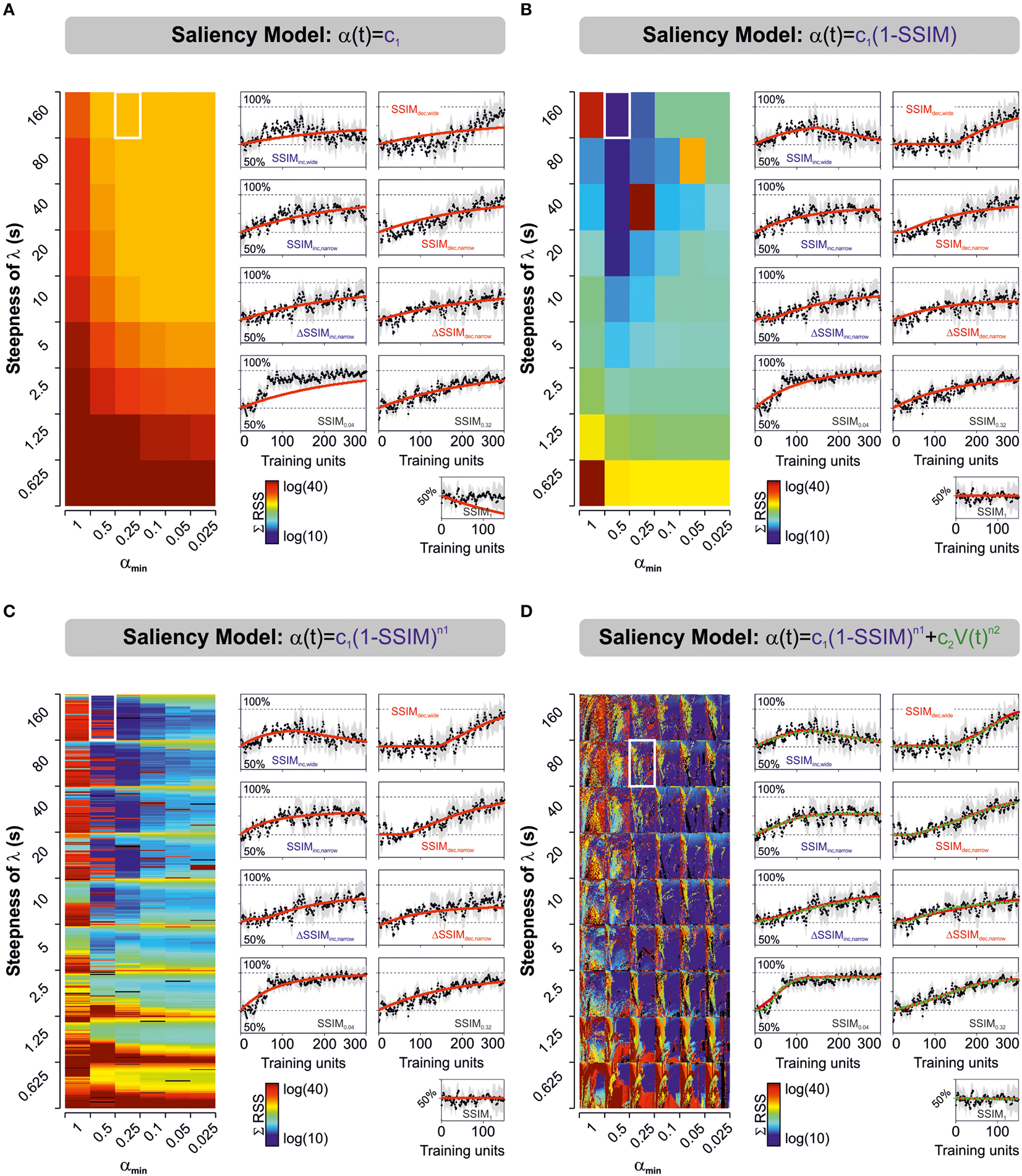
Figure 2. Predicted learning curves using different parameterizations for stimulus salience. Predicted learning curves (red lines) fitted to the empirical average choice records from mice trained with varying and constant stimulus similarity. Salience was represented as either a simple constant (A), as a linear (B), or non-linear (C) function of stimulus similarity (SSIM), or as the sum of two non-linear functions, one dependent on stimulus similarity, and the other on V(t) (D). Color-maps display the sum of squares (ΣRSS) for all nine experimental groups (same color scale for all cases). In (C) we mapped for different values of n₁ (n₁ ≥ 0:0.1:6, y-axis), whereas in (D) we mapped for n₁ (y-axis) and n₂ (n₂ = 0:0.1:6; x-axis). Common to all groups: β, c₁, k₂, and α_min. In (D), the red and green lines correspond to the best “unbound” (0 > ϕ ≥ ∞; 0 > ε ≥ ∞) and “bound” (0 > ϕ ≥ 1; 0 > ε ≥ 1) solutions, respectively. The best parameter fits for the unbound solution were β = 0.0154; k₁ = 0.0014; V_min = 0.55; λ_max = [1, 0.97, 0.77, 0.95, 0.84, 0.85, 0.70, 0.90, 0.93]; s = 80; α_min = 0.25; c₁ = 0.3827; n₁ = 1.5; c₂ = [0.31, 4.01, 12.91, 2.15, 2.92, 1.41, 0.00, 3.36, 9.56]; n₂ = 6, whereas those for the bound solution were β = 0.0140; k₁ = 0.0014; V_min = 0.55; λ_max = [1, 0.95, 0.77, 0.95, 0.85, 0.86, 0.70, 0.90, 0.93]; s = 80; α_min = 0.25; c₁ = 0.6762; n₁ = 2.7; c₂ = [0.27, 4.57, 10.88, 2.30, 2.64, 1.08, 0.00, 3.63, 7.11]; n₂ = 5.6. The arrangement of the panels with the learning curves is identical to the one described for Figures 1C,D.

To compare the “goodness of fit” among the different models, we adopted the Akaike Information Criterion [AIC (Burnham and Anderson, 2002)]. The AIC is a metric that seeks a model with a high-quality fit to the observed values, yet with as few free parameters as possible. The second order AIC (AICc) compensates for sample size by increasing the relative penalty for fits with small data sets:

$\begin{array}{ll}{AIC}_C=n·ln\left(\frac{RSS}{n}\right)+2K+\frac{2K\left(K+1\right)}{\left(n-K-1\right)}& (10)\end{array}$

where RSS is the residual sum of squares between the model and the empirical data, n is the number of observations (i.e., sample size), and K is the number of free parameters. We ranked all models by taking the best approximation with the lowest (most negative) AIC_C value. Next, we calculated the ΔAICc as the difference between the best model (smallest AICc) and the AIC_C for each model (i.e., the best model has a ΔAIC_C of zero). Finally, to calculate the Akaike weights (w_i), we took the relative likelihood of each prediction and divided it by the sum of these values across all models, as follows:

$\begin{array}{cc}{w}_i=\frac{e^{-\text{0}.\text{5}·△AI{C}_C}}{{\displaystyle {\sum }_{r=1}^R{e}^{-\text{0}.\text{5}·△AI{C}_{C,r}}}}& \left(11\right)\end{array}$

These weights had a normalized value falling between 0 and 1, corresponding to the probability that a given model becomes the best approximation and with the sum of all weights being 1. Overall, these coefficients take into account how well the model fits the data (using the RSS), favoring descriptions with fewer free parameters, as it penalizes the number of fitted parameters (K).

We displayed results as averages ± S.E.M and employed parametric and non-parametric statistical tests with a significance set at p < 0.05.

Results

Learning Curves for Mice Trained with Varying Similarity

We trained mice to learn to discriminate combinations of CS⁺/CS⁻ images (Figure 1A). The stimuli offered varying degrees of structural similarity (SSIM; Wang et al., 2004; Treviño et al., 2013; Figure 1B). The ${\text{CS}}_{\text{i}}^{-}$ stimuli were either exchanged on every trial or remained fixed during acquisition (Figure 1C). The first two experimental groups were trained with stimuli sorted with increasing (SSIM_{inc, wide}; Figure 1C₁, blue dots) or decreasing (SSIM_{dec, wide}; Figure 1C₂, red dots) similarity values. That is, this training consisted of sustained positive or negative SSIM gradients ranging from −0.07 to 1. The SSIM_{inc, wide} group displayed an initial growth in its average correct choice level, peaking at 88.5 ± 9.3% around the middle of training and then decreasing when SSIM > 0.30 (Figure 1D₁). By contrast, the decreasing similarity group (SSIM_{dec, wide}) displayed a slower onset of correct choice behavior and higher maximal performance of 98.7 ± 9.2% (Figure 1D₂).

We next trained two additional groups of mice (SSIM_{inc, narrow}: Figure 1C₃ and SSIM_{dec, narrow}: Figure 1C₄) in which the maximum similarity was kept below SSIM = 0.39. This training ensured that CS⁺/CS⁻ discriminability remained fully uncompromised during acquisition (Treviño et al., 2013). The correct choice level reached a plateau at maximal performance in the SSIM_{inc, narrow} group (Figure 1D₃) while the SSIM_{dec, narrow} group displayed a slower onset for correct choice and a higher average peak performance at the end of training (Figure 1D₄). We also tested training mice with increasing (ΔSSIM_{inc, narrow}: Figure 1C₅) or decreasing (ΔSSIM_{dec, narrow}: Figure 1C₆) oscillating gradients in similarity. Both ΔSSIM groups displayed similar learning rates and maximum performance (Figure 1D_5,6).

Finally, we trained mice with a fixed similarity of SSIM_0.04 = 0.04 (Figure 1C₇), SSIM_0.32 = 0.32 (Figure 1C₈), and SSIM₁ = 1 (Figure 1C₉). These groups allowed us to investigate how different, but fixed similarities, led to specific learning rates and peak discrimination performances (Rescorla and Wagner, 1972). As expected, the SSIM₁ mice failed to learn to discriminate (Figure 1D₉), but the other two groups showed increasing learning rates when trained with SSIM_0.32 (Figure 1D₈) and SSIM_0.04 (Figure 1D₇), respectively. Therefore, the learning rate increased by lowering stimulus similarity whereas shape and maximum retention level of the learning curves were determined by the sign and slope of the SSIM gradients during training (Treviño et al., 2013). Also, the changes in choice performance through learning were slow and retained across daily sessions (Karni and Sagi, 1993). The learning curves illustrated in Figure 1D were described in detail previously (Treviño et al., 2013) and serve as the empirical reference or “ground truth” for the mathematical analyses performed in the following sections.

Testing Multiple Representations for Stimulus Salience

We aimed to explore how the changes in stimulus similarity during acquisition could explain the empirically observed learning curves (Figure 1D). We used a simple linear operator model of associative learning aiming to predict the evolution of the associative strength (V(t); Bush and Mosteller, 1951; Rescorla and Wagner, 1972; Treviño et al., 2011). Our adaptation of this core predictive model includes important considerations. It assumes that the discrimination process does not lead to learning when stimulus salience is below a minimum effective salience threshold [α(t) ≤ α_min, V(t) < V_min]. Yet, it will produce learning when α(t) > α_min. Also, we defined the asymptote of learning (λ) as a sliding logistic function of α (see Materials and Methods), as proposed previously (Treviño et al., 2011). We did so because we reasoned that the quality of sensory representation should degrade gradually as the salience reaches α_min, compromising discrimination and learning (Treviño et al., 2011, 2013). The resulting equations predict that, at any given trial, the change in V(t) will be proportional to the product of the CS⁺/CS⁻ and the US saliencies acting linearly on the difference between the asymptote of learning [λ(α)] and V(t) (see Materials and Methods). In the simplest case, if α were a constant, V(t) would increase in a negatively accelerated manner, as V(t) approached λ(α) (Rescorla and Wagner, 1972).

One remarkable feature of our experimental data set is the fact that we changed the stimulus similarity during training (Groups 1–6; Figure 1C). In the next sections, we will illustrate how we explored the predictive power of different mathematical representations for stimulus salience. More concretely: our main hypothesis was that the net stimulus salience could be represented as the sum of effective (ϕ) plus acquired (ε) components (Esber and Haselgrove, 2011). In the equations we used, the effective salience (ϕ) derived explicitly from the visual properties of the stimulus (i.e., a function of SSIM) whereas the acquired salience [ε(t)] depended on the reinforcement history (Mackintosh, 1975; Pearce and Hall, 1980).

We tested and compared the predictive power of six models that represented stimulus salience with different equations (see Materials and Methods). For the first three models, we defined the net salience as an effective salience component only [i.e., α(t) = ϕ(SSIM)]. We set such effective salience as being either a simple constant (Model 1; Rescorla and Wagner, 1972), or as a constant that depended linearly (Model 2), or non-linearly (Model 3) on stimulus similarity (SSIM; Mackintosh, 1975; Pearce and Hall, 1980; Le Pelley, 2004). This description for effective salience (ϕ) constitutes an objective approach to quantify the structural differences among visual stimuli (Wang et al., 2004; Treviño et al., 2013), and it is consistent with the fact that it should be positively correlated with α (Mackintosh, 1975). For the last three salience formulations, we added a second component representing the acquired salience (ε). Model 4 involved a linear (n₂ = 1) or a non-linear (n₂ ≠ 1) function of the amount of learning [V(t)], allowing ε to grow monotonically with learning. Formally, this model implied that the ε would grow as a stimulus became a better predictor of an outcome (i.e., leading to a smaller prediction-error; Mackintosh, 1975). In contrast, for models 5 and 6, we defined ε in such a way that it would decrease with learning [because V(t) tends toward λ_max with training repetitions]. These two last models implied that the acquired salience would decrease with learning as the outcome of a trained stimulus became predictable (Pearce and Hall, 1980).

We employed non-linear programming techniques to fit all the models to the experimental data (see Materials and Methods). This approximation aimed to find those model parameters that minimized the residual sum of squares (RSS) between the experimental data and the model fits. We quantified the “goodness of fit” by applying the solver to the empirical learning curves from the nine experimental groups and then calculating the sum of RSS (ΣRSS) using different saliency descriptions (Figure 2). The color maps in Figure 2 illustrate the ΣRSS values mapped for different λ(α) slopes and α_min values. In some cases, we tested for various n₁ values (Model 3; n₁ = 0:0.1:6; Figure 2C) or the combination of multiple n₁ (y-axis) and n₂ values (x-axis; Model 4; n₁ = 0:0.1:6, n₂ = 0:0.1:6; Figure 2D). To enable valid comparisons, we applied the same color scale for all panels. The predicted learning curves (in red) correspond to the solutions that produced lowest ΣRSS for each model using “unbound” salience ranges (0 > ϕ ≥ ∞; 0 > ε ≥ ∞). The green dotted line in Figure 2D corresponds to the solution to Model 4 with ‘bound’ salience conditions (i.e., 0 > ϕ ≥ 1; 0 > ε ≥ 1). We provide the optimized parameters for the two best solutions in the legend of Figure 2. The predicted learning curves for salience models 5 and 6 are not illustrated.

A Model with Effective Plus Acquired Salience Predicts the Learning Curves

We used the second order Akaike Information Criterion (AICc) to compare and select the best description, from the models tested, for stimulus salience. Using an information theory approach (Burnham and Anderson, 2002), we seeked a model that presented a good fit to the observed data (Figure 3A), yet with as few free parameters as possible. This method also takes into account sample size by increasing the penalty for small data sets (see Materials and Methods). Finally, we calculated the Akaike weights (w_i) for each model (Table 2 and Figure 3B). Individual weights had a value between 0 and 1, corresponding to the probability that a given model constitutes the best approximation (Σw = 1), which thus provides a quantitative estimation of the relevance of the models under consideration. The saliency models 1, 2, 3, and 6 had minor Akaike weights (<1%). However, the fourth salience model captured the strongest weights with 27 ± 15% with unbound conditions and 56 ± 19% with bound conditions. The fifth model captured 16 ± 12% of the total weight (paired t-tests against models 1,2,3, and 6, *p < 0.05, **p < 0.01; Figure 3B). Therefore, the Model 4 (“bound” conditions) provided the best approximation from all models tested (One-way ANOVA multi-comparison test; F_{(6, 55)} = 4.80, p < 0.001).

FIGURE 3

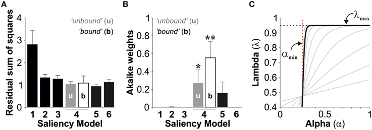
Figure 3. Best model selection. The bar plots display the group average residual sum of squares (A) and the Akaike weights (B) for the saliency models tested (Average ± S.E.M). (C) Plot of lambda vs. alpha using the best parameter fits described in Figure 2 (“bound” conditions). The pattern resembles a Heaviside step function suggesting that lambda does not depend on alpha.

TABLE 2

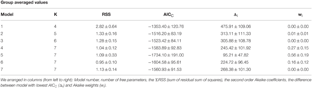
Table 2. Comparison of model fits with different free parameters.

We next solved lambda (Equation 9) by using the best parameter fits with the best model (model 4, bound conditions). The obtained relationship between lambda and alpha resembled a Heaviside step function indicating that these two variables are independent from each other (Figure 3C). Therefore, this means that we can treat lambda as a constant, yet this does not impair our conclusions because the equations we used to describe lambda covered this scenario (λ(α) → λ_max when s → ∞).

Evolution of Acquired Salience with Learning

The previous results revealed that a salience representation using effective plus acquired salience provided a better description of the learning curves compared to models considering the effective salience only. Yet, how does the acquired salience evolve with acquisition? Salience could increase or decrease depending on how good or bad a stimulus predicts its consequences (Mackintosh, 1975). Alternatively, the salience could decrease (or increase) as the stimulus becomes a better (or worse) predictor of its consequences (Pearce and Hall, 1980). To distinguish these two possible scenarios in our data, we solved the salience equations employing the best parameter fits with the best predictive model. In Figure 4, we illustrate the numeric solutions for the effective [ϕ(SSIM); left], acquired [ε(t); middle] and total salience [α(t) = ϕ(SSIM) +ε(t); right] with “unbound” (upper row; Figure 4A) and “bound” (lower row; Figure 4B) conditions. The trajectories for these saliency variables were quite similar for both solutions. As expected, the effective salience ϕ varied with an opposite slope with respect to changes in similarity (SSIM), because it is proportional to 1-SSIM (see Materials and Methods). The acquired salience, on the other hand, increased monotonically for all training programs except SSIM_{inc, wide} (Mackintosh, 1975). For this group, the acquired salience had a region of negative slope linked to the systematic drop in effective salience and the decay of V(t) (green arrow, Figures 4A,B, middle). As a result, almost for all groups, the total salience grew slowly (on average) because it consisted of the sum of effective plus acquired salience. Only the SSIM_{inc, wide} group had a minor portion with monotonic reduction in net salience, because it combined the decay for both the effective and the acquired salience. These results are consistent with the idea that the acquired salience grows as a stimulus becomes a better predictor of an outcome (Mackintosh, 1975).

FIGURE 4

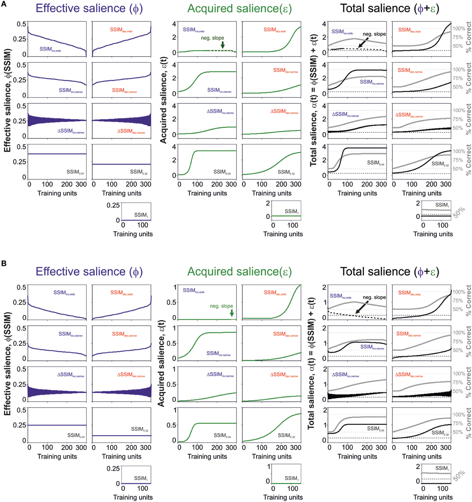
Figure 4. Changes in effective and acquired salience through training. Dynamic changes in effective (blue lines), acquired (green lines), and total (black lines) salience for the best predictive model parameters using “unbound” (0 > ϕ ≥ ∞; 0 > ε ≥ ∞; A) and “bound” (0 > ϕ ≥ 1; 0 > ε ≥ 1; B) salience conditions. The gray lines on the right panels correspond to the predicted associative strength curves.

The Learning Trajectory Determines the Maximum Acquired Salience

In this last section, we explored some of the possible predictions derived from the dual salience model. To do so, we defined a virtual training program based on two epochs. For the first epoch (trials 1–300), we used linear arrays of SSIM changing through discrete training steps (step-size = 1). These numbers represented training stimuli with different similarities yet the programs consisted of the same stimuli, sorted in ascending (blue), or descending (red) order, respectively. Note that subtracting these two scenarios maximizes the relative difference in SSIM between training programs. The second epoch (trials 301–600), consisted of training with constant SSIM ensuring a total salience above α_min. To simulate the discriminative learning, we took the virtual SSIM programs described above (Figure 5A) and, using the optimized parameters from the best predictive model (i.e., model 4 “bound” conditions), we solved Equation (1) by using the Runge-Kutta method with discretized time-steps (see Materials and Methods). We then extracted the values for the effective (Figure 5B), acquired (Figure 5C), and net (Figure 5D) saliencies, and also for the associative strength (Figure 5E). As expected, the temporal arrangement of SSIM determined the shape of the learning curves. When stimuli had a total salience below α_min, they were undetectable, V(t) did not increase, and the learning curves decayed toward chance level due to the lack of reinforcement [0 ≤ V(t) ≤ 1]. Notably, when similarity was held constant during the second epoch, the group trained with positive SSIM changes always performed below the group trained with negative SSIM gradients (Figure 5E). To further explore these differences, we took the peak values for the acquired and net saliencies observed during the first 300 trials (shaded region in the panels) and plotted them against the SSIM slope during training. Interestingly, although the maximum acquired salience was similar for the groups trained with positive and negative SSIM slopes (Figure 5F), the peak net salience was always bigger for negative (red lines) than for positive (blue lines) SSIM gradients (Figure 5G). This demonstrates that the differences in the trajectories in associative strength were due to the different arrangements of effective salience during training leading to a bigger net saliencies for the group trained with negative SSIM. Such differences in net salience provide a satisfactory explanation as to why the temporal arrangement of stimuli with the same effective salience can produce profoundly different learning curves (Treviño et al., 2013).

FIGURE 5

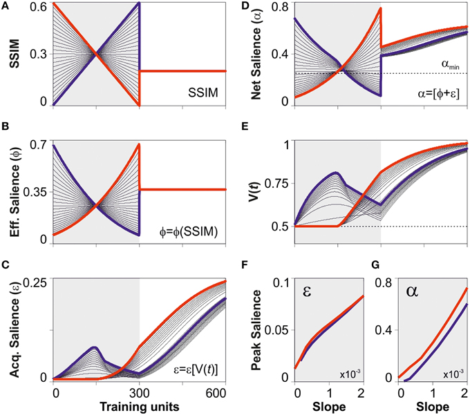
Figure 5. Differences in peak salience for training programs with identical stimuli. (A) Synthetic creation of SSIM training programs consisting of a variable SSIM epoch followed by a constant one. The first, “variable” epoch (from trial 1 to 300) was created using linear ramps with positive (blue) and negative (red) SSIM slopes. (B) These arrangements consist of the same stimuli, sorted in ascending (blue) or descending (red) order, respectively. The second, “constant” epoch (trials 301–600) consisted of training with the same constant SSIM, one that led to a net salience α(SSIM) > α_min. Solving Equation (7) (see Materials and Methods) we display the effective (B), acquired (C), and net (D) salience. To simulate discriminative training, we took the optimized parameters from the best predictive model displayed in Figure 2D (“bound” salience; green dotted line) and numerically solved Equation (1) (see Materials and Methods). We illustrate the predicted learning curves in panel (E). The overall differences in the learning curves can be explained by the differences in net (G) but not in acquired (F) peak salience during training.

Discussion

We adapted a mathematical model in order to predict the choice records from nine groups of mice trained with heterogeneous visual stimuli (Treviño et al., 2013). Specifically, we compared the predictive power of a simple associative learning rule coupled to six different saliency descriptions with the idea of gaining insight into the salience mechanisms involved in the learning process. Several studies have assumed that the contribution of the conditioned stimuli to learning is fixed (Bush and Mosteller, 1951; Rescorla and Wagner, 1972). Here, we explored a complementary view: we tested whether our empirical data could be explained by learning rules that involved a more flexible representation for stimulus associability, as suggested by other authors (Mackintosh, 1975; Pearce and Bouton, 2001; Le Pelley, 2004; Esber and Haselgrove, 2011). Indeed, we coupled our learning model to functions that allowed us to represent the stimulus salience in different relevant ways. By using the Akaike Information Criterion (AIC), we found that the best predictive model was one in which we defined the total salience as the sum of effective plus acquired components. The effective salience was a fixed quantity that depended only on the physical attributes of the stimuli whereas the acquired salience depended on how the associative strength changed during acquisition. This second component allowed the net salience to change as a result of learning about the outcome of the trained stimuli (Lawrence, 1949, 1950; Mackintosh, 1975; Esber and Haselgrove, 2011).

The exact definitions for effective and acquired saliencies were relatively unimportant to us because there are multiple other ways in which they could be formulated. Yet, we avoided some specific combinations of variables due to analytical reasons. For example, variables that are introduced into formulas as multiplicative factors are not structurally identifiable. This is because there is an infinite number of possible values that such variables could adopt to solve the mathematical problem: “a change in one parameter can be compensated by a proportional shift in the other one, still producing a satisfying fit between experimental data and model predictions” (Dochain and Vanrolleghem, 2001).

The structural similarity index (SSIM; Wang et al., 2004) constitutes a useful quantitative tool for assessing perceptual similarity both in humans (Wang et al., 2004) and mice (Treviño et al., 2013). We used this index to compare the similarity among images and defined the effective salience as a non-linear function of it. Moreover, we assumed that the effective salience of a stimulus could be represented by the salience of any other stimulus times the similarity between them (Mackintosh, 1975; Pearce, 1994; Treviño et al., 2011). This notion implied that the changes in associative strength were extracted through generalizations across stimuli (Lawrence, 1952; Shepard, 1987; Dosher and Lu, 2007; Cleland et al., 2009). Behavioral generalization is a process in which similar stimuli become associated with the same contingency and has been used to assess perceptual similarity in diverse animal models (Lawrence, 1949, 1952; Pearce, 1987; Shepard, 1987; Dosher and Lu, 2007). The psychometric function that describes how different stimuli group together is called generalization gradient and decreases with perceptual similarity distance (Shepard, 1987). It would be of particular interest to explore how the changes in effective salience during training influence the shape of the generalization gradient.

Many learning models propose that conditioned stimuli are processed with constant salience (v.gr. Rescorla and Wagner, 1972). In nature, however, salience is variable because context and experience change dynamically. Indeed, there is ample evidence that saliency signals depend on prior experience as they can be acquired via contiguity (Lawrence, 1949; Sutherland and Mackintosh, 1971). Recently, Esber and Haselgrove (2011) developed an attentional model based on effective (i.e., stimulus-driven) plus acquired salience. Inspired by their model, we defined our equations in such a way that the acquired salience would evolve with the associative history of trained stimuli (Mackintosh, 1975; Pearce, 2008; Esber and Haselgrove, 2011). This formulation allowed the net stimulus salience to grow or decay slowly, depending on how the subjects learned about the predictive power of the stimuli (i.e., the learning trajectory; Mackintosh, 1975). Our analytical results revealed that, as suggested previously, training with a fixed stimulus increased the acquired salience through learning (Mackintosh, 1975). One important implication of this explanatory frame is that stimuli with the same effective salience (i.e., identical stimuli) can have different net saliencies and vice versa (i.e., different stimuli having the same net salience).

Theories of selective attention propose that learning about a stimulus requires attending to that particular stimulus on the first place. They also claim that a spatial “saliency map” can describe the salience of an entire visual scene, allowing the detection of locations with distinctive visual attributes (Gottlieb et al., 1998; Itti and Koch, 2001). The activity of some neurons in the visual cortex is involved in the computation of elementary features of the stimulus including a “preliminary” saliency map (Itti and Koch, 2001; Li, 2002). Such an initial salience computation in the visual cortex is a “bottom-up”, stimulus-driven signal that contains information about how different is a stimulus from its surroundings (Koch and Ullman, 1985; Ahissar and Hochstein, 1993; Desimone and Duncan, 1995; Reynolds et al., 2000; Li, 2002; Baker et al., 2004; Gutnisky, 2009). Our results support this view that, indeed, the physical properties of a stimulus determine its initial salience, but then, along longer time scales, the stimulus salience will also evolve with experience. We propose that the effective stimulus salience is thus a perceptual consequence of a complex interaction of the target stimulus with other surrounding stimuli. This information is then processed by cortical sensory neurons, which change their response properties based on prior experience (Gilbert et al., 2009; Sasaki et al., 2010). Other brain areas involved in processing salience signals include the ventral visual pathway (Mazer and Gallant, 2003; Serences and Yantis, 2007), the frontal eye fields (FEF; Thompson and Bichot, 2005; Serences and Yantis, 2007), the orbitofrontal cortex (Lucantonio et al., 2012; Ogawa et al., 2013) and some subcortical structures such as the superior colliculus (SC; Kustov and Robinson, 1996) and the pulvinar (Robinson and Petersen, 1992).

A multitude of factors can trigger changes in stimulus salience. Rescorla and Wagner (1972) acknowledged the fact that the salience of a stimulus could decrease through pre-exposure to the stimulus. This pre-exposure effect to the CS⁺ is generally referred to as “latent inhibition” (LI) and has been demonstrated in a number of animal species (Lubow and Moore, 1959; Le Pelley, 2004). One common interpretation for LI is that it arises from a reduced stimulus salience as a result of an experience with the stimulus without consequence in the non-reinforced “pre-exposure” phase (Lubow and Moore, 1959). Such a reduction in the learning rate produced by LI could reflect the capacity of individuals not to attend to, or to ignore, stimuli that predict no significant consequences (Weiner, 2003). Interestingly, LI is disrupted in rodents injected with amphetamines (which promote dopamine [DA] release) leading to psychotic symptoms, and this is reversed by treatment with antipsychotic drugs (which potentiate LI). Pharmacological disruption LI is thus considered to provide an animal model of some of the symptoms of schizophrenia (Weiner, 2003).

To make optimal decisions, animals must integrate information about their previous actions and compare them with their current needs (Lucantonio et al., 2012). They are particularly receptive to events that violate their expectations, which in turn facilitate associative learning (Mackintosh, 1975; Pearce and Bouton, 2001). Such a mismatch between expectancy and experience constitutes a prediction-error, driving learning through the allocation of attention to specific stimuli in the environment (Rescorla and Wagner, 1972; Mackintosh, 1975). Prediction errors and expectancies of reward are represented by midbrain DA neurons (Schultz, 2013) which send projections to the prefrontal and orbitofrontal cortices (Gottfried et al., 2003; Corlett et al., 2007; Mainen and Kepecs, 2009). A current proposal is that a dysregulated, hyperdopaminergic state in patients with psychiatric disorders like schizophrenia (and also in drug addiction), leads to disrupted prediction-error processing and aberrant assignment of salience. From this point of view, psychotic states are preceded by an exaggerated release of DA providing motivational significance to irrelevant stimuli (Kapur, 2003; Corlett et al., 2007; Lucantonio et al., 2012). Notably, psychostimulant agents that trigger DA release (v.gr. amphetamines) are associated with de novo psychosis, whereas antipsychotics that reduce DA transmission, assist in the resolution of the symptoms (Kapur, 2003; Weiner, 2003). For these reasons, we believe that understanding how salience is acquired will be a fundamental step to understand sensory information processing in normal and pathological conditions. The analytical tools that we developed in this work could enable the characterization of aberrant salience acquisition in animal models of schizophrenia.

Author Contributions

MT conceived, designed and performed the data analysis. MT made figures and wrote the manuscript.

Funding

Support was provided from the Mexican Consejo Nacional de Ciencia y Tecnología (CONACYT: 220862, 07384, 251406).

Conflict of Interest Statement

The author declares that the research was conducted in the absence of any commercial or financial relationships that could be construed as a potential conflict of interest.

Acknowledgments

We thank Dr. Rafael Gutiérrez for critical comments to the manuscript; E. Aguilar-Garnica and L. Sanchez-Carrasco for useful suggestions; R. Gutiérrez and E. Matute for constant support.

References

Ahissar, M., and Hochstein, S. (1993). Attentional control of early perceptual learning. Proc. Natl. Acad. Sci. U.S.A. 90, 5718–5722. doi: 10.1073/pnas.90.12.5718

PubMed Abstract | CrossRef Full Text | Google Scholar

Baker, C. I., Olson, C. R., and Behrmann, M. (2004). Role of attention and perceptual grouping in visual statistical learning. Psychol. Sci. 15, 460–466. doi: 10.1111/j.0956-7976.2004.00702.x

PubMed Abstract | CrossRef Full Text | Google Scholar

Burnham, K. P., and Anderson, D. R. (2002). Model Selection and Multimodel Inference; A Practical Information-theoretic Approach. New York, NY; Berlin; Heidelberg: Springer-Verlag.

Google Scholar

Bush, R. R., and Mosteller, F. (1951). A mathematical model for simple learning. Psychol. Rev. 58, 313–323. doi: 10.1037/h0054388

PubMed Abstract | CrossRef Full Text | Google Scholar

Cleland, T. A., Narla, V. A., and Boudadi, K. (2009). Multiple learning parameters differentially regulate olfactory generalization. Behav. Neurosci. 123, 26–35. doi: 10.1037/a0013991

PubMed Abstract | CrossRef Full Text | Google Scholar

Corlett, P. R., Murray, G. K., Honey, G. D., Aitken, M. R., Shanks, D. R., Robbins, T. W., et al. (2007). Disrupted prediction-error signal in psychosis: evidence for an associative account of delusions. Brain 130, 2387–2400. doi: 10.1093/brain/awm173

PubMed Abstract | CrossRef Full Text | Google Scholar

Desimone, R., and Duncan, J. (1995). Neural mechanisms of selective visual attention. Annu. Rev. Neurosci. 18, 193–222. doi: 10.1146/annurev.ne.18.030195.001205

PubMed Abstract | CrossRef Full Text | Google Scholar

Dochain, D., and Vanrolleghem, P. (2001). Dynamical Modelling and Estimation in Wastewater Treatment Processes. London: IWA publishing.

Google Scholar

Dosher, B. A., and Lu, Z. L. (2007). The functional form of performance improvements in perceptual learning: learning rates and transfer. Psychol. Sci. 18, 531–539. doi: 10.1111/j.1467-9280.2007.01934.x

PubMed Abstract | CrossRef Full Text | Google Scholar

Esber, G. R., and Haselgrove, M. (2011). Reconciling the influence of predictiveness and uncertainty on stimulus salience: a model of attention in associative learning. Proc. Biol. Sci. 278, 2553–2561. doi: 10.1098/rspb.2011.0836

PubMed Abstract | CrossRef Full Text | Google Scholar

Gilbert, C. D., Li, W., and Piech, V. (2009). Perceptual learning and adult cortical plasticity. J. Physiol. 587, 2743–2751. doi: 10.1113/jphysiol.2009.171488

PubMed Abstract | CrossRef Full Text | Google Scholar

Gottfried, J. A., O'Doherty, J., and Dolan, R. J. (2003). Encoding predictive reward value in human amygdala and orbitofrontal cortex. Science 301, 1104–1107. doi: 10.1126/science.1087919

PubMed Abstract | CrossRef Full Text | Google Scholar

Gottlieb, J. P., Kusunoki, M., and Goldberg, M. E. (1998). The representation of visual salience in monkey parietal cortex. Nature 391, 481–484. doi: 10.1038/35135

PubMed Abstract | CrossRef Full Text | Google Scholar

Griffiths, O., and Mitchell, C. J. (2008). Selective attention in human associative learning and recognition memory. J. Exp. Psychol. Gen. 137, 626–648. doi: 10.1037/a0013685

PubMed Abstract | CrossRef Full Text | Google Scholar

Gutnisky, D. A., Hansen, B. J., Iliescu, B. F., et al. (2009). Attention alters visual plasticity during exposure-based learning. Curr. Biol. 19, 555–560. doi: 10.1016/j.cub.2009.01.063

PubMed Abstract | CrossRef Full Text | Google Scholar

Harris, J. A. (2006). Elemental representations of stimuli in associative learning. Psychol. Rev. 113, 584–605. doi: 10.1037/0033-295X.113.3.584

PubMed Abstract | CrossRef Full Text | Google Scholar

Herrera, D., and Trevino, M. (2015). Undesirable choice biases with small differences in the spatial structure of chance stimulus sequences. PLoS ONE 10:e0136084. doi: 10.1371/journal.pone.0136084

PubMed Abstract | CrossRef Full Text | Google Scholar

Itti, L., and Koch, C. (2001). Computational modelling of visual attention. Nat. Rev. Neurosci. 2, 194–203. doi: 10.1038/35058500

PubMed Abstract | CrossRef Full Text | Google Scholar

Jiang, Y., and Chun, M. M. (2001). Selective attention modulates implicit learning. Q. J. Exp. Psychol. A 54, 1105–1124. doi: 10.1080/713756001

PubMed Abstract | CrossRef Full Text | Google Scholar

Kapur, S. (2003). Psychosis as a state of aberrant salience: a framework linking biology, phenomenology, and pharmacology in schizophrenia. Am. J. Psychiatry 160, 13–23. doi: 10.1176/appi.ajp.160.1.13

PubMed Abstract | CrossRef Full Text | Google Scholar

Karni, A., and Sagi, D. (1993). The time course of learning a visual skill. Nature 365, 250–252. doi: 10.1038/365250a0

PubMed Abstract | CrossRef Full Text

Koch, C., and Ullman, S. (1985). Shifts in selective visual attention: towards the underlying neural circuitry. Hum. Neurobiol. 4, 219–227.

PubMed Abstract | Google Scholar

Kustov, A. A., and Robinson, D. L. (1996). Shared neural control of attentional shifts and eye movements. Nature 384, 74–77. doi: 10.1038/384074a0

PubMed Abstract | CrossRef Full Text | Google Scholar

Lawrence, D. H. (1949). Acquired distinctiveness of cues; transfer between discrimination on the basis of familiarity with the stimulus. J. Exp. Psychol. 39, 770–784. doi: 10.1037/h0058097

PubMed Abstract | CrossRef Full Text | Google Scholar

Lawrence, D. H. (1950). Acquired distinctiveness of cues: selective association in a constant stimulus situation. J. Exp. Psychol. 40, 175–188. doi: 10.1037/h0063217

PubMed Abstract | CrossRef Full Text | Google Scholar

Lawrence, D. H. (1952). The transfer of a discrimination along a continuum. J. Comp. Physiol. Psychol. 45, 511–516. doi: 10.1037/h0057135

PubMed Abstract | CrossRef Full Text | Google Scholar

Le Pelley, M. E. (2004). The role of associative history in models of associative learning: a selective review and a hybrid model. Q. J. Exp. Psychol. B 57, 193–243. doi: 10.1080/02724990344000141

PubMed Abstract | CrossRef Full Text | Google Scholar

Li, Z. (2002). A saliency map in primary visual cortex. Trends Cogn. Sci. 6, 9–16. doi: 10.1016/S1364-6613(00)01817-9

PubMed Abstract | CrossRef Full Text | Google Scholar

Lubow, R. E., and Moore, A. U. (1959). Latent inhibition: the effect of nonreinforced pre-exposure to the conditional stimulus. J. Comp. Physiol. Psychol. 52, 415–419. doi: 10.1037/h0046700

PubMed Abstract | CrossRef Full Text | Google Scholar

Lucantonio, F., Stalnaker, T. A., Shaham, Y., et al. (2012). The impact of orbitofrontal dysfunction on cocaine addiction. Nat. Neurosci. 15, 358–366. doi: 10.1038/nn.3014

PubMed Abstract | CrossRef Full Text | Google Scholar

Mackintosh, N. J. (1975). A theory of attention: variations in the associability of stimuli with reinforcement. Psychol. Rev. 82, 276–298.

Google Scholar

Mainen, Z. F., and Kepecs, A. (2009). Neural representation of behavioral outcomes in the orbitofrontal cortex. Curr. Opin. Neurobiol. 19, 84–91. doi: 10.1016/j.conb.2009.03.010

PubMed Abstract | CrossRef Full Text | Google Scholar

Mazer, J. A., and Gallant, J. L. (2003). Goal-related activity in V4 during free viewing visual search. Evidence for a ventral stream visual salience map. Neuron 40, 1241–1250. doi: 10.1016/S0896-6273(03)00764-5

PubMed Abstract | CrossRef Full Text | Google Scholar

McFarland, D. J. (1971). Feedback Mechanisms in Animal Behaviour. London: Academic Press Inc.

Google Scholar

Ogawa, M., van der Meer, M. A., Esber, G. R., et al. (2013). Risk-responsive orbitofrontal neurons track acquired salience. Neuron 77, 251–258. doi: 10.1016/j.neuron.2012.11.006

PubMed Abstract | CrossRef Full Text | Google Scholar

Pearce, J. M. (1987). A model for stimulus generalization in Pavlovian conditioning. Psychol. Rev. 94, 61–73. doi: 10.1037/0033-295X.94.1.61

PubMed Abstract | CrossRef Full Text | Google Scholar

Pearce, J. M. (1994). Similarity and discrimination: a selective review and a connectionist model. Psychol. Rev. 101, 587–607. doi: 10.1037/0033-295X.101.4.587

PubMed Abstract | CrossRef Full Text | Google Scholar

Pearce, J. M. (2008). Animal Learning & Cognition, 3rd Edn. New York, NY: Psychology Press.

Pearce, J. M., and Bouton, M. E. (2001). Theories of associative learning in animals. Annu. Rev. Psychol. 52, 111–139. doi: 10.1146/annurev.psych.52.1.111

PubMed Abstract | CrossRef Full Text | Google Scholar

Pearce, J. M., and Hall, G. (1980). A model for Pavlovian learning: variations in the effectiveness of conditioned but not of unconditioned stimuli. Psychol. Rev. 87, 532–552. doi: 10.1037/0033-295X.87.6.532

CrossRef Full Text | Google Scholar

Rescorla, R. A., and Wagner, A. R. (1972). “A theory of Pavlovian conditioning: variations in the effectiveness of reinforcement and non reinforcement,” in Classical Conditioning II: Current Research and Theory, eds A. H. Black and W. F. Prokasy (New York, NY: Appleton-Century-Crofts), 64–99.

Reynolds, J. H., Pasternak, T., and Desimone, R. (2000). Attention increases sensitivity of V4 neurons. Neuron 26, 703–714. doi: 10.1016/S0896-6273(00)81206-4

PubMed Abstract | CrossRef Full Text | Google Scholar

Robinson, D. L., and Petersen, S. E. (1992). The pulvinar and visual salience. Trends Neurosci. 15, 127–132. doi: 10.1016/0166-2236(92)90354-B

PubMed Abstract | CrossRef Full Text | Google Scholar

Roelfsema, P. R., van Ooyen, A., and Watanabe, T. (2010). Perceptual learning rules based on reinforcers and attention. Trends Cogn. Sci. 14, 64–71. doi: 10.1016/j.tics.2009.11.005

PubMed Abstract | CrossRef Full Text | Google Scholar

Sasaki, Y., Nanez, J. E., and Watanabe, T. (2010). Advances in visual perceptual learning and plasticity. Nat. Rev. Neurosci. 11, 53–60. doi: 10.1038/nrn2737

PubMed Abstract | CrossRef Full Text | Google Scholar

Schultz, W. (2013). Updating dopamine reward signals. Curr. Opin. Neurobiol. 23, 229–238. doi: 10.1016/j.conb.2012.11.012

PubMed Abstract | CrossRef Full Text | Google Scholar

Serences, J. T., and Yantis, S. (2007). Spatially selective representations of voluntary and stimulus-driven attentional priority in human occipital, parietal, and frontal cortex. Cereb. Cortex. 17, 284–293. doi: 10.1093/cercor/bhj146

PubMed Abstract | CrossRef Full Text | Google Scholar

Shepard, R. N. (1987). Toward a universal law of generalization for psychological science. Science 237, 1317–1323. doi: 10.1126/science.3629243

PubMed Abstract | CrossRef Full Text | Google Scholar

Sutherland, N. S., and Mackintosh, J. (1971). Mechanisms of animal Discrimination Learning. New York, NY: Academic Press.

Google Scholar

Thompson, K. G., and Bichot, N. P. (2005). A visual salience map in the primate frontal eye field. Prog. Brain Res. 147, 251–262. doi: 10.1016/S0079-6123(04)47019-8

PubMed Abstract | CrossRef Full Text | Google Scholar

Treviño, M. (2014). Stimulus similarity determines the prevalence of behavioral laterality in a visual discrimination task for mice. Sci. Rep. 4:7569. doi: 10.1038/srep07569

PubMed Abstract | CrossRef Full Text | Google Scholar

Treviño, M., Aguilar-Garnica, E., Jendritza, P., Li, S. B., Oviedo, T., Köhr, G., et al. (2011). Discrimination learning with variable stimulus ‘salience’. Int. Arch. Med. 4:26. doi: 10.1186/1755-7682-4-26

PubMed Abstract | CrossRef Full Text | Google Scholar

Treviño, M., Frey, S., and Kohr, G. (2012). Alpha-1 adrenergic receptors gate rapid orientation-specific reduction in visual discrimination. Cereb. Cortex 22, 2529–2541. doi: 10.1093/cercor/bhr333

PubMed Abstract | CrossRef Full Text | Google Scholar

Treviño, M., Oviedo, T., Jendritza, P., Li, S. B., Köhr, G., and De Marco, R. J. (2013). Controlled variations in stimulus similarity during learning determine visual discrimination capacity in freely moving mice. Sci. Rep. 3:1048. doi: 10.1038/srep01048

PubMed Abstract | CrossRef Full Text | Google Scholar

Wang, Z., Bovik, A. C., Sheikh, H. R., and Simoncelli, E. P. (2004). Image quality assessment: from error visibility to structural similarity. IEEE Trans. Image Process. 13, 600–612. doi: 10.1109/TIP.2003.819861

PubMed Abstract | CrossRef Full Text | Google Scholar

Weiner, I. (2003). The “two-headed” latent inhibition model of schizophrenia: modeling positive and negative symptoms and their treatment. Psychopharmacology (Berl). 169, 257–297. doi: 10.1007/s00213-002-1313-x

PubMed Abstract | CrossRef Full Text | Google Scholar