Reading as active sensing: a computational model of gaze planning in word recognition

Introduction

The human visual system is essentially active, its processing strategies being tightly coupled with the specific demands of an ongoing task (Yarbus, 1967 ; Ballard, 1991 ; Johansson et al., 2001 ; O’Regan and Nöe, 2001 ). There is ample evidence that in everyday activities, such as driving, walking or reading, gaze shifts are used to gather task-relevant information (Triesch et al., 2003 ; Hayhoe and Ballard, 2005 ; Land, 2006 ). Whenever possible, this is done through efficient, timely selection of the specific information required for a given stage of the task to be carried out, with no need to store information (Ballard et al., 1995 ). In most tasks, since visual information is required at the very early stages of action planning, the strategy gives rise to anticipatory saccades (e.g., by fixating objects that are manipulated shortly later, or even seconds later).

One visual task that has been the focus of intense investigation is text reading. Somewhat contrary to commonsense, it does not consist in the serial fixation of written words from left-to-right, but it is a truly active task. In reading a text, some words are skipped, and occasionally a gaze regression is made to words that were either already fixated, or skipped. Patterns of eye movements (including, among other things, the time spent on each fixation and the average distance the eyes move along while scanning a text) are complex and depend on a number of factors, including word frequency, lexical predictability and ambiguity, complexity in the syntactic structure of input text etc. (see Rayner, 2009 for a recent review).

In line with this evidence, the present paper intends to investigate the interlocked relationship between processes of self-organizing lexical storage and learning on the one hand, and, on the other hand, active sensing strategies for reading that exploit expectations on stored lexical representations to drive gaze planning. For this purpose, we shall capitalize on currently emerging views on morphological processing and on the role of anticipatory processes in reading.

Word processing has recently been conceptualized as the outcome of simultaneously activating patterns of cortical connectivity, reflecting (possibly redundant) distributional regularities in the input at the graphemic, morpho-syntactic and morpho-semantic levels (Burzio, 2004 ; Baayen, 2007 ; Post et al., 2008 ). This view argues for a more complex and differentiated neurobiological substrate for human language than both classical dual-route (Pinker and Prince, 1988 ; Prasada and Pinker, 1993 ; Pinker and Ullman, 2002 ; Ullman, 2004 ) and connectionist one-route models (McClelland and Patterson, 2002 ; Westermann and Plunkett, 2007 ) can posit. Brain areas devoted to word processing appear to maximize the opportunity of using both general and specific information simultaneously (Libben, 2006 ), rather than maximize processing efficiency and economy of storage.

Topological models of lexical self-organization can shed light on such a dynamic view of word processing from a computational perspective (Pirrelli, 2007 ; Pirrelli et al., in press ). In these models, lexical storage and learning is based on the concurrent self-organization of “spatial” word-based information (e.g. segmental or graphemic patterns) and temporal (i.e. sequential) information, accounting for concomitant effects of redundant morphological structure and predictive parsing, as well as for short-term and long-term memory effects in the encoding and processing of symbolic sequences. This makes spatio-temporal self-organizing networks of this kind ideally suitable for investigating anticipatory processes in word recognition and reading.

Experimental studies based on ERP (event-related potentials) and eye-movement evidence show that people use prior (lexical and semantic) contextual knowledge to anticipate upcoming words (Altmann and Kamide, 1999 ; Federmeier, 2007 ). DeLong et al. (2005) demonstrate that expected words are pre-activated in subjects’ brain in a graded fashion, reflecting their expected probability. This body of evidence provides a solid empirical ground to the probabilistic approach to lexical prediction and gaze planning proposed here. In our model, the probability distribution of stored lexical representations is the main input to the gaze planner, since (parts of) words predicted with high accuracy can be skipped safely during reading (as demonstrated empirically by Ehrlich and Rayner, 1981 ; Rayner and Well, 1996 ). Moreover, new information that is (retrospectively) judged as unpredictable and surprising can determine longer fixations, regressions, or revision of lexical representations.

The aforementioned evidence provides the foundations of our modeling approach to gaze planning, in which two components interact: a lexical representation network, and a gaze planner proper. We offer a model of how lexical representations and lexical predictions can be exploited as a basis for an active reading strategy, and analyze the developmental trajectory of the system in a word recognition task as a function of increasing lexical competence and lexical prediction ability. It is worth noting that the interactions between (predictive) learning of task representations and active sensing strategies during task learning and execution are not confined to the linguistic domain, addressed here, but are characteristic of a wide variety of sensorimotor tasks: hence the interest of our approach in developmental robotics studies in general.

Materials and Methods

Model Architecture and Components

Our gaze planning model consists of a lexical representation network, and the gaze planner proper. The lexical representation network is implemented as a Temporal Hebbian Self-Organizing Map (THSOM; Koutnik, 2007 ), an extension of Kohonen’s Self-Organizing Maps (SOMs; Kohonen, 2001 ) that, in addition to developing topological patterns of input data, models their temporal sequences and supports prediction.

Based on the input provided by a THSOM trained on written words, the gaze planner implements an active sensing strategy for reading. The model actively selects where the next fixation should be placed, rather than passively scanning all text input, from left-to-right at an even pace. We model the problem of planning gaze sequences in reading as a Bayesian sequential decision process. The eye/gaze controller plans an optimal active sensing strategy (under uncertainty) by weighting up future (lexical) information gain and costs. In particular, our target function is to maximize the (expected) information gain (i.e., how much new lexical information is gained through each gaze), minimize the amount of uncertainty in lexical representations (i.e., disambiguate between competing words, say, “house” and “horse”), and minimize costs (i.e., time spent, effort required for short and long saccades). We tested the gaze planner at different stages of lexical acquisition and analyzed the developmental trajectories of eye-movement patterns as a function of (i) the growing lexical complexity of input text, and (ii) the level of reader’s lexical competence modeled by a THSOM. Our gaze planning algorithm was eventually compared with two (Bayesian) strategies that use complete information on word statistics.

The Lexical Network

(Topological) Temporal hebbian self-organizing map (T⁽²⁾HSOM)

SOMs define a class of unsupervised clustering algorithms that mimic the behavior of medium to small aggregations of neurons in the cortical area of the brain, involved in the specialized processing of classes of sensory data. Processing in such neural aggregations (called brain maps) consists in the activation (or firing) of one or more neurons, each time a particular stimulus is presented. A crucial feature of brain maps is their topological organization (Penfield and Rasmussen, 1950 ; Penfield and Roberts, 1959 ): nearby neurons in the map are fired by similar stimuli. Although some brain maps are taken to be genetically pre-programmed, there is evidence that at least some aspects of such global neural organization emerge as a function of the sensory experience accumulated through learning (Kaas et al. 1983 ; Jenkins et al. 1984 ). Functionally, brain maps are thus dynamic memory stores, directly involved in input processing, and exhibiting effects of dedicated long-term topological organization.

A THSOM is a SOM augmented with a temporal connection layer (Figure 1 ). Classical components of a SOM are parallel processing nodes (or receptors) arranged in a grid or map. Each node in the map is synaptically connected with all elements of the input layer, where input vectors are encoded. Each connection is treated as a communication channel with no time delay, whose synaptic strength is modeled by a weight value. Each receptor is thus associated with one space weight vector defined on the spatial connection layer. We distinguish here the input space, staked out by the defining dimensions of the input layer, from the map space, i.e. the (usually two-dimensional) grid where receptors are spatially located.

FIGURE 1

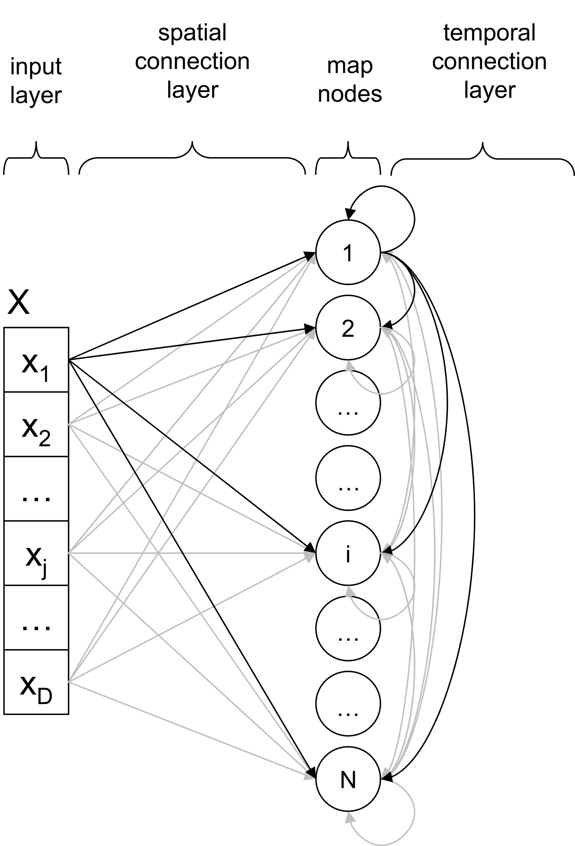
Figure 1. Architecture of a THSOM.

In a classical SOM, learning is measured in time steps, with each step corresponding to exposure to a single stimulus token. A time step includes three phases: input encoding, input activation and input learning. When a stimulus is encoded on the input layer, all map nodes are activated in parallel as a function of how close their weights are to values of the current input vector. Learning consists in adjusting weights on the spatial connection layer for them to get closer to the corresponding values on the input layer. Weight adjustment does not apply evenly across map nodes and time steps, but depends on similarity to the input vector, learning rate and space topology. At each time step, the most strongly adjusted node is the most highly firing one, or Best Matching Unit (BMU). All other nodes are adjusted as a function of their distance from BMU on the map (or neighborhood function). Weights of nodes that lie close to BMU are made more similar to input values than weights of nodes lying further away from BMU. After adjustment, the time step counter is increased by one tick, the map activation is reset and another input stimulus is encoded. Both learning rate (α) and neighborhood function (ν) vary through time to simulate the behavior of a brain map losing its plasticity.

A THSOM models synchronization between two BMUs firing at consecutive time steps. This means that a THSOM can remember, at time t, its state of activation at time t−1 and can make an association between the two states. This is possible by augmenting traditional SOMs with an additional layer of synaptic connections between each single node and all other nodes on the map (Figure 1 ). For each node, this defines a further association with a time weight vector. Connections on this layer (referred to in Figure 1 as the temporal connection layer) are treated as communication channels whose synaptic strength is modeled by a weight value updated with a fixed one-step time delay. Weights on the temporal layer are adjusted with a Hebbian learning strategy (Hebb, 1949 ) based on activity synchronization of BMU at time t−1 and BMU at time t.

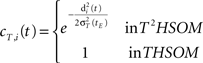
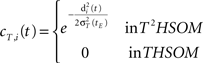
During training, the temporal connection between the two BMUs is potentiated (Figure 2 A), while the temporal connections between all other nodes and BMU at time t are depressed (Figure 2 B). Logically, this amounts to enforcing the entailment BMU_t → BMU_t−1. Finally, unlike classical SOMs, the level of activation of a THSOM node at time t is determined by the summation of two vector distances: the distance between the current input vector and the node’s space weight vector (as in traditional SOMs), and the distance between the node’s time weight vector and the state of activation of the whole map at time t−1.

FIGURE 2

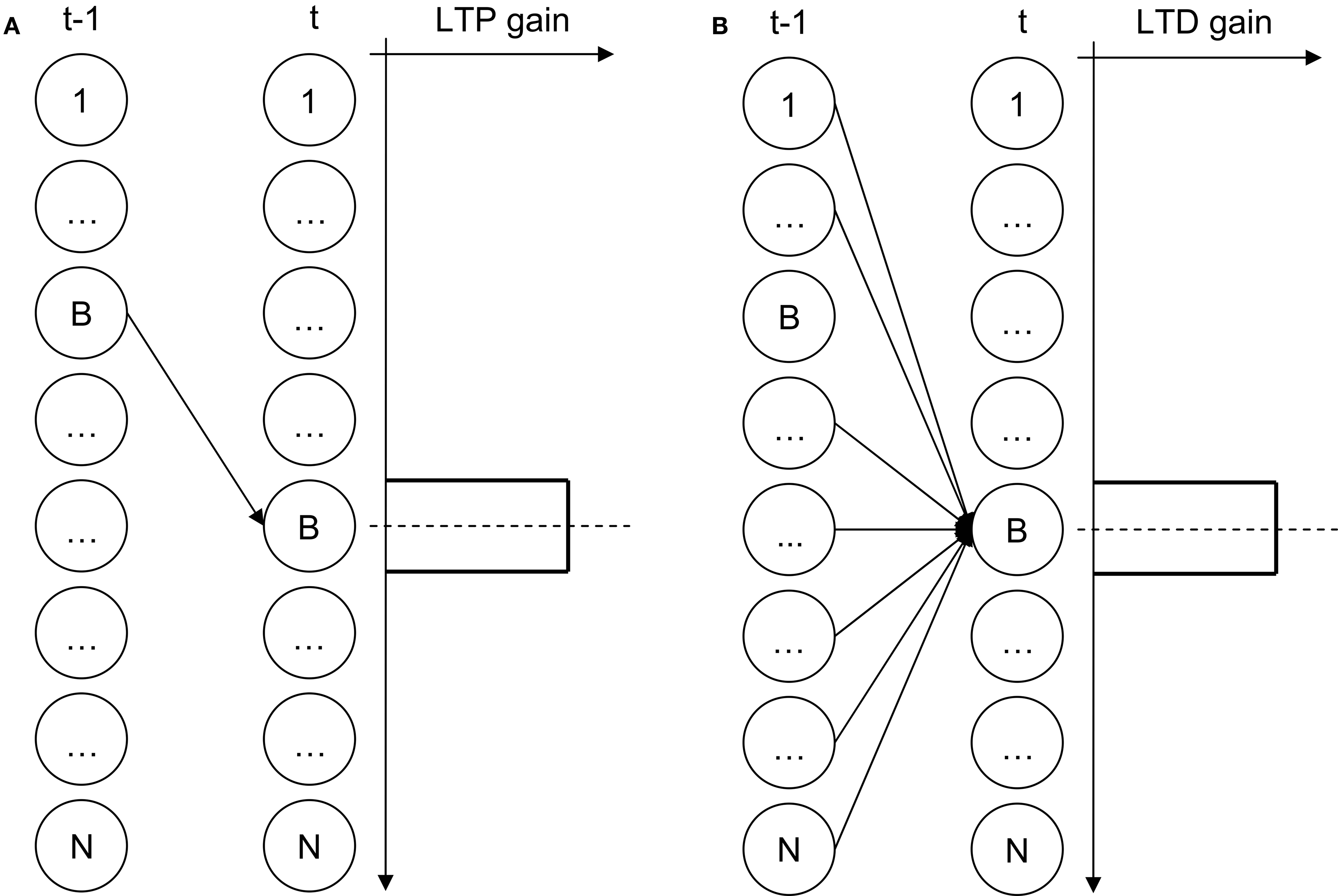
Figure 2. THSOM temporal layer plasticity. (A) potentiation; (B) depression.

When trained on time series of input vectors, a THSOM develops (i) a topological organization of receptors by their sensitivity to similar input vectors (or spatial similarity) and (ii) a first-order time-bound correlation between BMUs activated at two consecutive time steps.

Knowledge of a trained THSOM is stored in the synaptic weights of its nodes. We can calibrate the map by assigning a label to each map node. A label is the input symbol which the node is most sensitive to, that is whose input vector matches the node’s space vector best. Labeling reveals the topological coherence of the resulting organization (Figure 4 ). Receptors that are fired by similar input vectors tend to stick together in the map space. Large areas of receptors are recruited for frequently occurring input vectors. In particular, if the same input vector occurs in different contexts, the map tends to recruit specialized receptors that are sensitive to the specific contexts where the input vector is found. The more varied the distributional behavior of an input vector, the larger the area of dedicated receptors (space allowing).

This dynamics is coherent with a learning strategy that minimizes entropy over inter-node connections. For each map node n_j, we transform connection weights into transition probabilities by simply normalizing the weight of a single outgoing (post-synaptic) connection by the summation of the weights over all outgoing connections from n_j. The resulting transition matrix is used to analyze the performance of the model at recall and in particular: (1) the entropy level of each node according to Shannon and Weaver’s equation; (2) variation in the entropy of an input sequence as it unfolds its activation over the map; (3) the ability of the map to predict an input sequence, expressed in terms of average (un)certainty in guessing the next transition.

We shall return to a detailed analysis of these aspects later in the paper. Suffice it to say at this juncture that the topological dynamics of a map constrains the degree of freedom to recruit dedicated receptors, as all receptors compete for space on the map. As a result, low-frequency input vectors may lack dedicated receptors after training. By the same token, dedicated receptors may generalize over many instances of the same input vector, gaining in generality but losing in modeling their distributional behavior. The main consequence of a poor modeling of the time-bound distribution of input vectors is an increasing level of entropy, as more context-free nodes present more post-synaptic connections. However, topological generalization is essential for a map to learn symbolic sequences whose complexity exceeds the map’s memory resources (i.e. the number of available nodes). Moreover, lack of topological organization makes it difficult for a large map to converge on learning simple tasks, as the map has no pressure to treat identical input tokens as instances of the same type.

Pirrelli et al. (in press) originally extend Koutnik’s THSOM architecture by using the neighborhood function as a principle of organization of connections on the temporal connection layer (Figures 3 A,B). An additional depressant Hebbian rule penalizes the temporal connections between BMU at time t−1 and all nodes lying outside the neighborhood of BMU at time t (Figure 3 C). This is equivalent to the logical entailment BMU_t−1 → BMU_t. Taken together, the temporal connections depicted in Figure 3 enforce a bi-directional entailment between BMU_t−1 and BMU_t inducing a bias for biunique first-order Hebbian connections. THSOMs that are augmented with this bias are called Topological Temporal Hebbian Self-Organizing Map (T²HSOM).

FIGURE 3

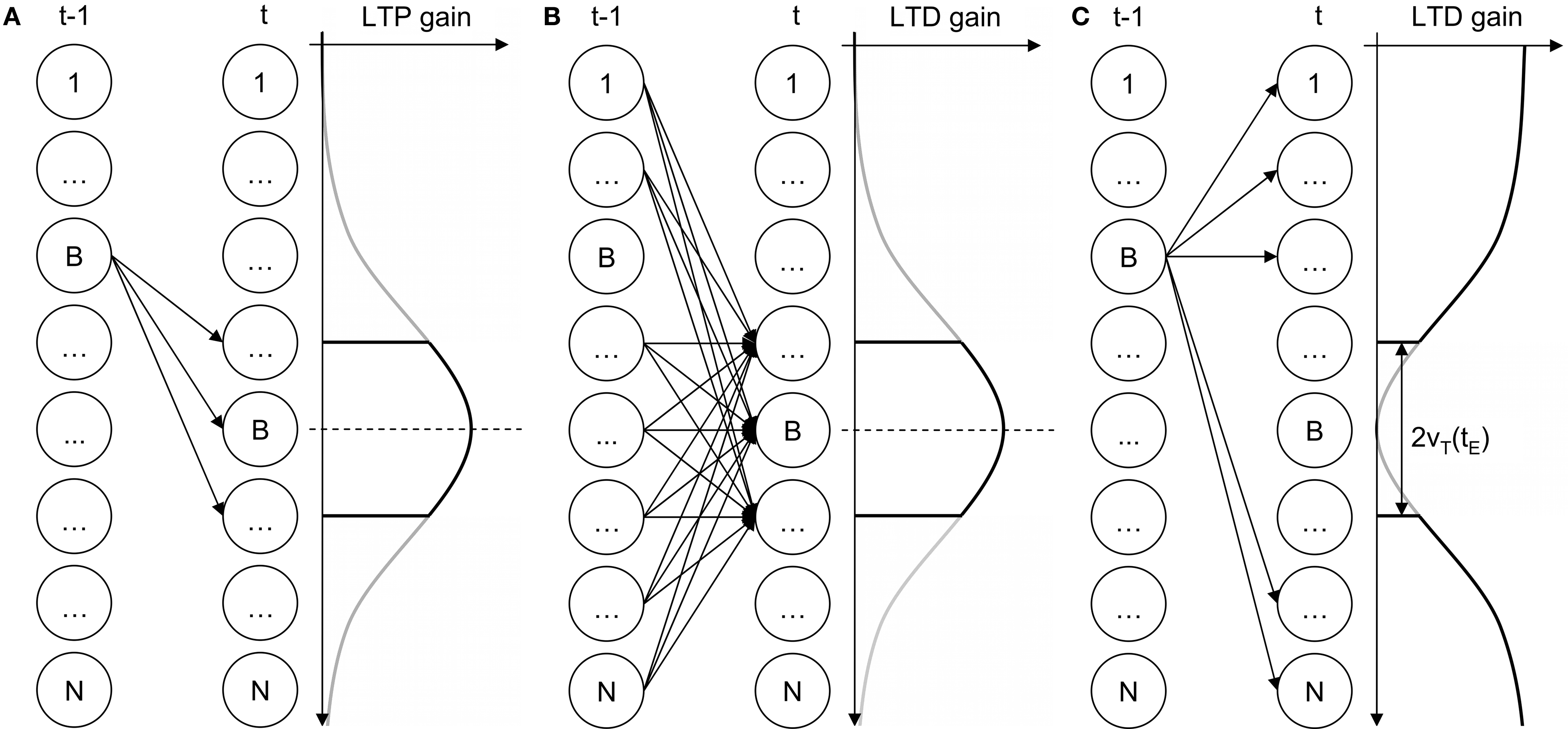
Figure 3. T²HSOM temporal layer plasticity. (A) potentiation; (B,C) depression.

In T²HSOM, input vectors can be similar for two independent and potentially conflicting reasons: (i) they have vector representations that are close in the input space; (ii) they distribute similarly, i.e. they tend to be found in similar sequences. Unlike a THSOM, which is sensitive to space similarity only, a T²HSOM tries to optimize topological clustering according to both criteria for similarity at the same time. Pirrelli and colleagues show that the dynamic cooperation/competition between the two criteria for similarity is instrumental in capturing paradigmatic effects in the topological organization of the morphological lexicon.

To sum up this long excursus, the overall organization of a T⁽²⁾HSOM ¹ after training can be characterized as follows: (1) if space allows, one topologically connected cluster is present for each symbol; for lack of space, receptors can act as abstract states, fired by a class of similar symbols; (2) receptors that are sensitive to similar symbols are close on the map; (3) the temporal distribution of a symbol may carve out hierarchical sub-clusters within the main cluster for that symbol; (4) the size of a cluster depends on both frequency and the temporal distribution of the corresponding symbol. In the following section we illustrate how T⁽²⁾HSOM can be used to develop lexical representations.

Building a lexical network with a T⁽²⁾HSOM

A T⁽²⁾HSOM can learn word forms as time series of alphabetic characters flanked on either side by a start-of-word symbol (‘#’) and an end-of-word symbol (‘$’), as in “#,F,A,C,C,I,O,$”.

At each time step, the map is exposed to one single character in its left-to-right order of appearance. Upon exposure to the end-of-word symbol ‘$’, the map resets its Hebbian connections thus losing memory of the correlation between two consecutive word forms. In fact, word forms are repeatedly presented to the map in a random order as a function of their frequency in the training data set. Such a deliberately simplified version of the language learning task helps the map to focus on aspects of word-internal structure, abstracting away from other potentially confounding factors.

By being trained on several lexical sequences of this kind, a T⁽²⁾HSOM (i) develops internal representations of alphabetic characters, (ii) connects them through first-order Hebbian links, (iii) clusters developed representations topologically. The three steps are not taken one after the other but dynamically interact in non trivial ways. From a logical view point, step (i) corresponds to learning individual symbols by recruiting specialized receptors that are increasingly more sensitive to one symbol or class of symbols. Generally speaking, low-frequency symbols are slower in recruiting dedicated receptors than high-frequency symbols are. Step (ii) allows the map to develop selective paths through consecutively activated BMUs. This corresponds to learning word forms or recurrent parts of them. Once more, this is a function of the frequency with which symbol sequences are presented to the map. Finally, step (iii) uses either spatial information only (THSOMs) or both spatial and temporal information (T²HSOMs) to cluster nodes topologically. Accordingly, nodes that compete for the same symbol stick together on the map. Moreover, they tend to form sub-clusters to reflect distributionally different instances of the same symbol. For example, the symbol A in “#,F,A,C,C,I,O,$” (faccio, ‘I do’) will fire, if space allows, a different node than the same symbol in “#,S,E,M,B,R,A,$” (sembra, ‘it seems’).

An example of a trained lexical map is shown in Figure 4 . The map is calibrated, with each node being labeled by the alphabetic character that most strongly activates it. Arrows pictorially represent synaptic connections between consecutively activated BMUs. In the figure, shades of grey represent different transition probabilities (connection weights), from black (high values) to light grey (low values).

FIGURE 4

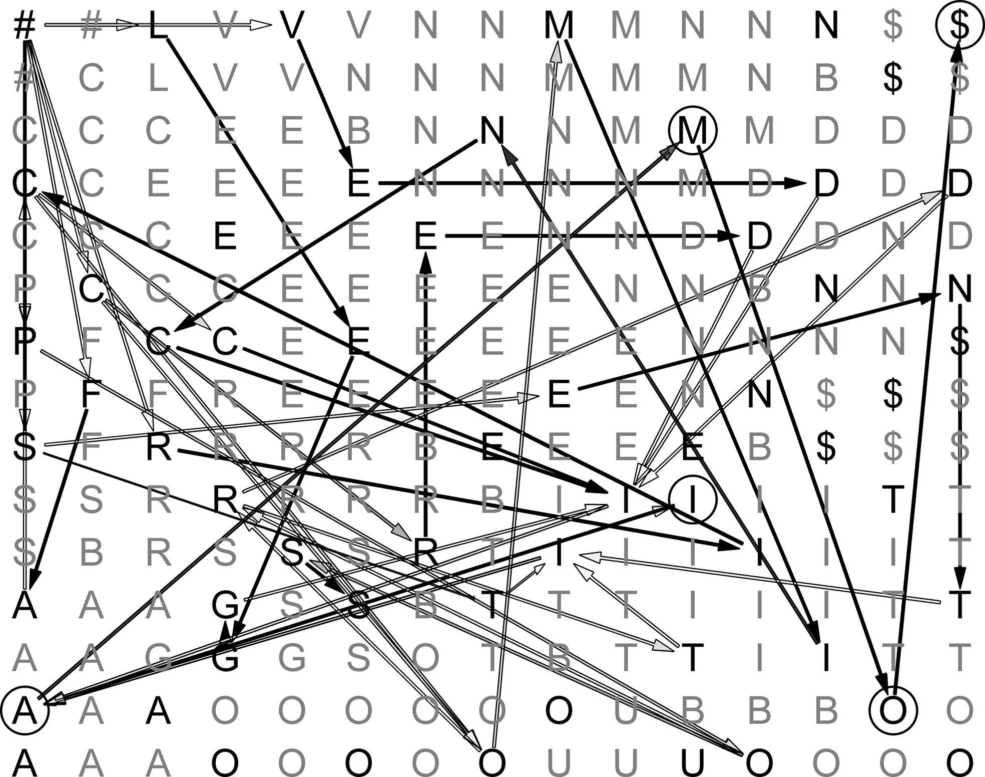
Figure 4. Sample map during learning. Darker edges represent more probable transitions, and lighter edges represent less probable ones.

In some cases, it is possible to follow a continuous path of connections going from ‘#’ (start-of-word) to ‘$’ (end-of-word). Only high-frequency word forms, however, are associated with a full path of inter-node connections after training. In the vast majority of cases, only recurring subsequences of activated nodes show strong connection patterns. These may correspond to inflectional endings (such as “I,A,M,O,$” in the figure), verb stems or parts of them.

Gaze Planning in Reading: A Bayesian Ideal-Observer Perspective

The second component of our model is the gaze planner. A gaze planner can be conceptualized as a Bayesian ideal-observer, i.e. “a theoretical device that performs a given task in an optimal fashion, given the available information and some specified constraints” (Geisler, 2003 , p. 825) spelled out in the framework of Bayesian statistical decision theory. In this framework, one typically assumes that in vision tasks humans behave as (approximate) optimal Bayesian decision makers. Alternatively, one can use the ideal-observer perspective to derive an optimal strategy, without assuming that humans use it, and compare human performance against it with the objective to discover analogies and differences.

In Bayesian analysis, one important aspect of information acquisition is the reduction of uncertainty over the variables that are relevant to the task at hand (e.g., location of objects in space, and/or their orientation, etc.). Reduction of uncertainty is not only valuable per se, but also in connection with action execution and behavioral decisions to be taken in the task. This aspect is captured by the notion of value of information (Howard, 1966 ): information has a value, which depends on the extent to which it is expected to disambiguate alternative beliefs and (particularly) make behavioral choice effective. That is, new information that could prompt a decision change is more valuable. By estimating the expected value of gazes, a system can select the gaze planning strategy that maximizes the value of acquired information (Sprague and Ballard, 2003 ; Nelson and Cottrell, 2007 among others).

To design our gaze planning algorithms, we drew inspiration from the Bayesian ideal-observer analysis. Here ‘task knowledge’ consists in lexical representations, and the task to be performed is recognizing written words in a text by reading a variable number of characters from left-to-right. Note that word recognition is simpler than reading, as only the latter requires a grapheme-to-phoneme mapping function. In word recognition, a Bayesian ideal-observer strategy makes use of lexical predictions to estimate the expected value gain of prospective gazes. This is conducive to gaze plans that aim to maximize such gain under time constraints and in the presence of uncertainty. On the basis on this general idea, we tested three gaze planning algorithms.

Algorithm 1

The first algorithm implements a simplified prediction-based procedure, which consists in skipping all characters that can be predicted reliably (i.e., above a given threshold) by a T⁽²⁾HSOM.

All characters (with the exception of the start-of-word symbol ‘#’) making up a written input word are initially masked by ‘*’. For example, at the outset, the word “#,F,A,C,C,I,O,$” is shown to the gaze planner as the string ‘#,*,*,*,*,*,*,*’. The algorithm starts from the first unmasked character ‘#’ and looks into a trained T⁽²⁾HSOM for a set of (probabilistic) predictions over all ‘#’-ensuing characters. This is done by looking at the most highly activated node (BMU) when the input symbol ‘#’ is shown to the map, and by inspecting the set of current BMU’s post-synaptic connections (i.e. its outgoing transitions). The gaze planner then decides whether the coming written character(s) should be skipped or not depending on how accurate the T⁽²⁾HSOM’s prediction(s) are. If the highest weight of a BMU’s post-synaptic connection (say ‘#’ → ‘C’) is above a set threshold, then an input character is skipped in reading and the gaze planner takes ‘C’ as the next input character. If no post-synaptic weight exceeds the threshold, control is returned to reading and the ensuing written character is unmasked. When the system reaches the end-of-word symbol ‘$’, then the sequence of guessed/read symbols is returned and evaluated against the current input word.

Note that the gaze planner is provided with a fovea that fixates only one character at a time (there being no periphery). In other terms, each landing position provides information about one character at a time. Due to the absence of periphery, the system cannot use the strategy that appears to be the most widely used by human readers, i.e., planning the landing positions around the word center (with an additional systematic error, which might derive from Bayesian estimation; see Engbert and Krügel, 2010 ). For the sake of simplicity, we further assume here that there are no landing errors, and that gazed characters are perfectly recognized. The algorithm, intended to focus on the importance of prediction, is not only (computationally) simpler than minimizing vocabulary entropy (as in Algorithm 3 below), but takes into account at the same time reduction of uncertainty and sequential nature of the reading task, without introducing motor costs for planning saccades of different amplitude (i.e. longer saccades are more costly for the motor system to execute, and more noisy on average).

Algorithms 2 and 3

Like Algorithm 1, Algorithm 2 scans an input word from left-to-right, starting from the first symbol and trying to make predictions about the upcoming characters on the basis of information on their immediate predecessor. Transition probabilities are estimated here through complete statistical information about the distribution of characters in the full training lexicon. If transition probabilities exceed a set threshold, a prediction is made and the corresponding letter in the input word is skipped. If the guessed character is not ‘$’, then a novel belief about another upcoming character is entertained, based on the previously guessed information.

Algorithm 3 makes no full left-to-right scanning of the input text and tries to minimize the number of reading steps required to identify the full word correctly. At each reading step, it places the gaze upon that position in the input string associated with the lowest possible entropy score. Entropy here is defined as a function of the number (and frequency) of outstanding word candidates that remain to be evaluated once the character in the selected position is read off. Suppose, for the sake of concreteness, that the lexicon is made up out of two strings only, say ABC and ABD. In this case, to establish which of the two words is currently input, reading either the first or the second character would not minimize entropy, as it does not reduce the number of possible candidates. Only the character in third position would reduce uncertainty to zero and thus represents the optimal character to be gazed at. In realistic scenarios, at each reading step new entropic scores are estimated on the basis of a shrinking set of candidate words, until one candidate word only is left.

Results and Discussion

The three algorithms were tested in two different experiments. For all of them, we used the same set of training data. Training data and testing data were identical in all reported simulations.

Experiment 1

We tested the Algorithm 1 from Section “Gaze planning in reading: a Bayesian ideal-observer perspective”, where gaze planning is based on the capacity of a trained T⁽²⁾HSOM to predict written lexical representations. A THSOM and a T²HSOM were independently trained on the same set of Italian written verb forms and results on both trials were compared. Both SOMs were bi-dimensional square grids of 25 × 25 nodes.

Training materials

The training data set contained distinct present indicative forms of 10 Italian verbs, for a total of 66 different forms, whose frequency distributions were sampled from the Calambrone section of the Italian CHILDES sub-corpus (MacWhinney, 2000 ), of about 110,000 token words. The average word length was 6.5 characters (see the frequency distribution in Figure 7 A). Forms were mostly selected from regular, formally transparent morphological paradigms. Nonetheless, some subregular high-frequency forms were introduced in the training set to monitor their representational trajectories during learning.

Written forms were represented as sequences of alphabetic characters between ‘#’ and ‘$’. To train the lexical network, alphabetic characters were encoded through a distributed, grapheme-based representation consisting of a 20-element vector, with each element encoding a specific feature of the graphical rendering of orthographic symbols cast into the grid of Figure 5 .

FIGURE 5

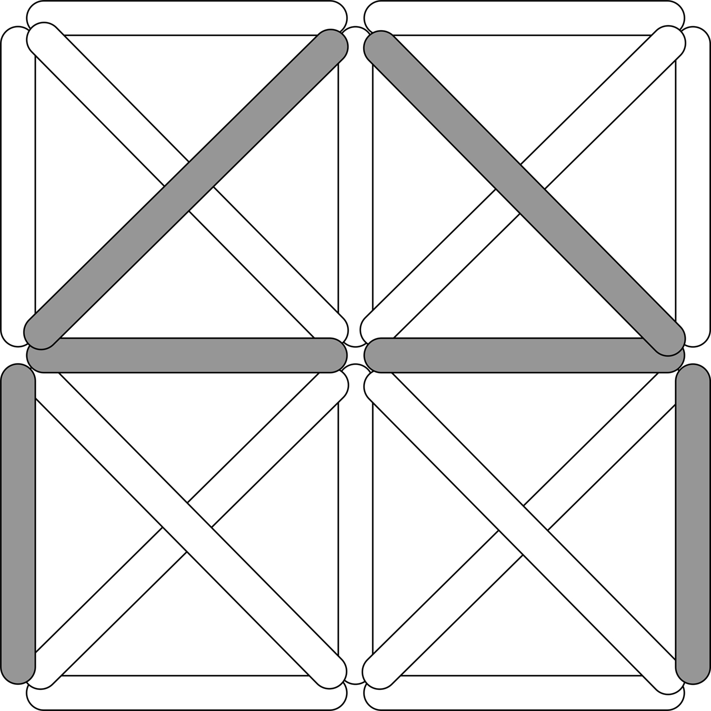
Figure 5. Representation of a capital “A” in the graphical grid.

Training protocol

Lexical network. Both maps were trained over 100 epochs. For each epoch, the training data set was treated as an urn containing verb forms. In the urn, the number of (identical) verb forms of the same type reflected the frequency of the verb type in our reference corpus. One verb form at a time was drawn from the urn, and its spelling retrieved. Each character in the spelling was converted into a distributed grapheme-based input vector and was shown to a T⁽²⁾HSOM in its order of appearance. When the ‘$’ symbol of the current input word form was shown, the internal clock of the map was reset and the word discarded. Another word was then drawn from the lexical urn and the whole training process was repeated over again until the urn was emptied.

Gaze planner. The same set of verb forms used for training the SOMs was then used for testing the gaze planner. Word forms are presented as dynamically unmasked sequences of characters (see “Gaze planning in reading: a Bayesian ideal-observer perspective”).

Figure 6 shows the results of the two networks in the word recognition task, broken down by learning epochs (which is also an indirect evaluation of the topological organization of the trained SOMs, see Pirrelli et al., in press ). The values reported in Figure 6 are averaged over repeated (10) experiments for each network. In particular, we measured the algorithm’s accuracy rate (the percentage of words that were identified correctly) and prediction rate (the percentage of characters that were predicted, not necessarily correctly, and thus skipped in reading) over 100 learning epochs, by plotting them against increasing levels of confidence (x axis). Low levels of confidence indicate that the gaze planner has a tendency to skip characters even though they are not strongly predicted by the network connections. Higher confidence thresholds correspond to a more conservative attitude towards reading, whereby only highly predictable ensuing characters are skipped. Clearly, lower thresholds yield less accurate results (the ascending solid line in the panels) and higher percentages of guessed symbols (descending dashed line in the panels).

FIGURE 6

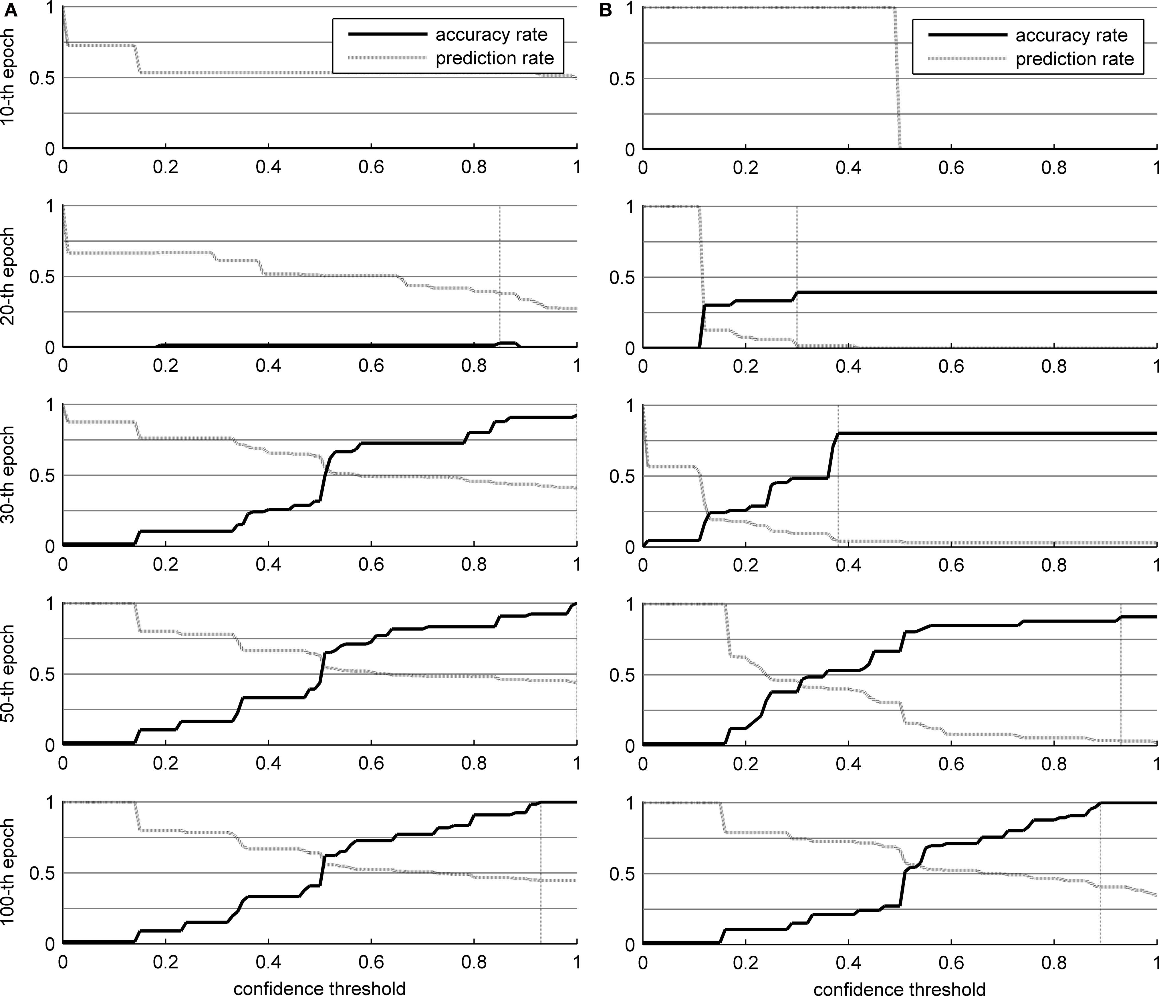
Figure 6. Results of the word identification experiment for 66 words in the corpus. The vertical dotted line indicates the optimal confidence threshold. (A) THSOM model; (B) T²HSOM model.

Careful analysis of the developmental trajectories of both models throws some notable phenomena in relief. Both models increase their overall accuracy rate as learning progresses. At the beginning, there are no specialized receptors for each character in the alphabet. Hence, networks are not able to recognize every single character. For instance, it might happen that a ‘C’ is presented to a network, but the corresponding BMU is labeled as a ‘G’. This explains the poor performance in the first 20 epochs, even when almost all characters are read. In addition, over the first 30 epochs, transition probabilities are too low to be used effectively, and nearly every character has to be read.

Observe the different developmental stages the two networks go through (Figure 6 ). Both maps converge on full scale accuracy rates (i.e. 100%) and comparable prediction rates, with Koutnik’s THSOM averaging 44.7% per word prediction at a 0.93 level of confidence, and the T²HSOM scoring 40.6% per word prediction at 0.89, after 100 learning epochs. Note, however, that Koutnik’s THSOM converges remarkably more quickly than T²HSOM. THSOM exhibits a tendency to retain longer stretches of input words at a faster pace than T²HSOM, as shown by the overall number of saccades of varying length in the two models (Figures 7 B,C respectively). The reason for this behavior lies in the capacity of THSOMs to “pack” more nodes that are competing for the same symbol in a comparatively smaller area of the map. Recall that, in T²HSOMs, competing receptors strongly inhibit each other and can coexist only at a distance. The same constraint does not hold for THSOMs, where context-sensitive receptors of the same symbol do not fight for short-range survival. A wider range of context-sensitive receptors minimizes the number of post-synaptic connections, thereby minimizing per node entropy and facilitating memorization of longer symbol chains.

FIGURE 7

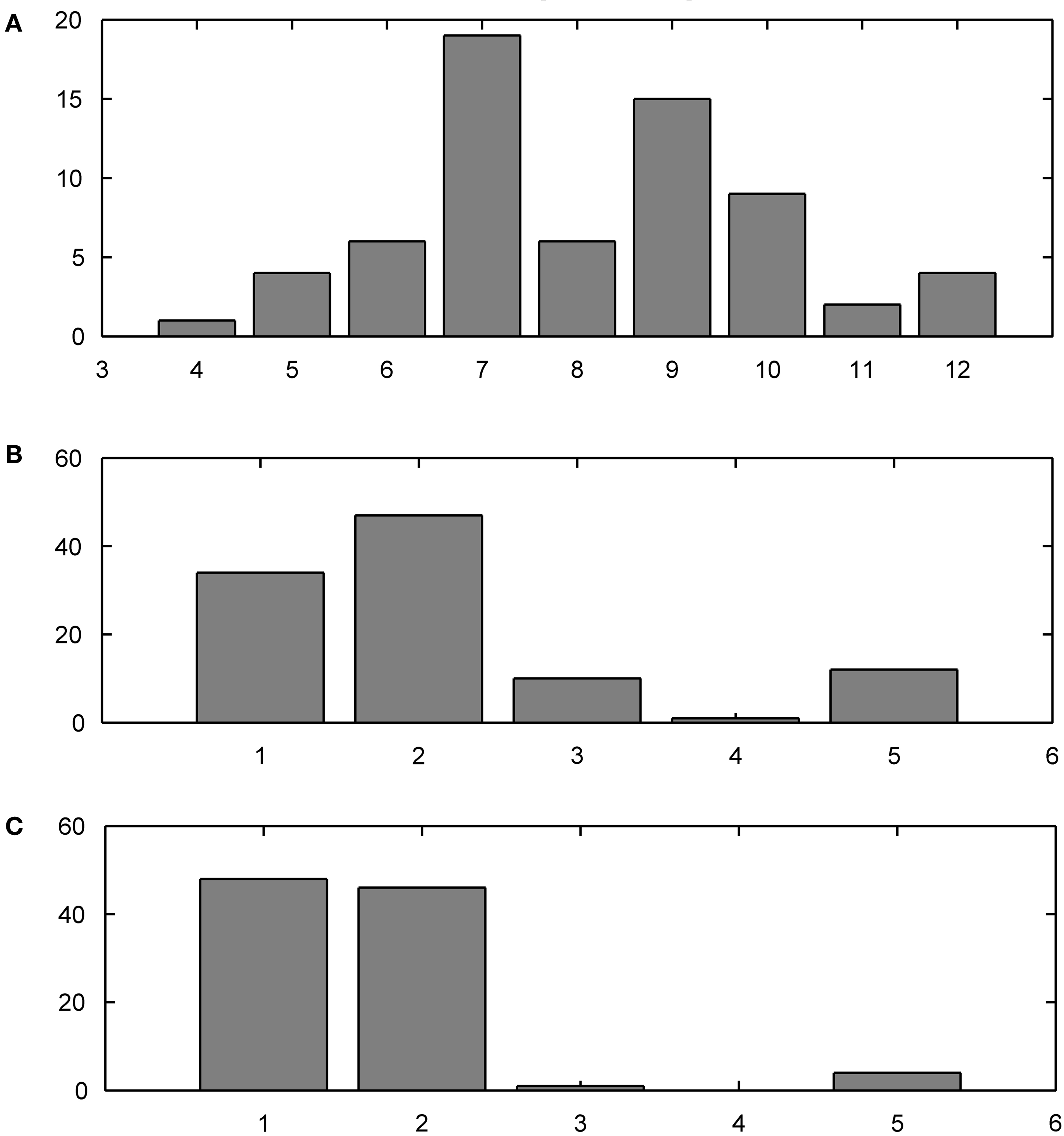
Figure 7. Training corpus word frequency histogram (A) and saccade frequency histogram test results; (B) THSOM model; (C) T²HSOM model.

On the other hand, strong competition between symbol tokens in complementary distribution is helpful in learning morphological structure. Tested on the task of identifying morpheme boundaries within inflected forms, the two maps show a reversed accuracy pattern: T²HSOMs are consistently better at finding morpheme transitions than THSOMs are. A 15 × 15 nodes T²HSOM is able to identify morpheme boundaries with 71% accuracy, while a THSOM of the same size has an accuracy of 64% on the same task and test data. Once more, when map size increases, accuracy scores of the two maps level out. Figure 8 shows transition probabilities at morpheme boundaries in the present indicative forms of the verb CREDERE (‘believe’), plotted against learning epochs. In a THSOM (Figure 8 A) lack of inhibition between complementarily distributed endings blots out the difference in frequency distribution among them. On the other hand, a T²HSOM proves to be sensitive to the uneven distribution of forms in the paradigm (Figure 8 B). This is shown to have important consequences in learning and access of lexical representations in human speakers (Baayen, 2007 ) and is demonstrably related to levels of difficulty in reading morphologically complex words by dyslexic and non dyslexic subjects (Burani et al., 2008 ).

FIGURE 8

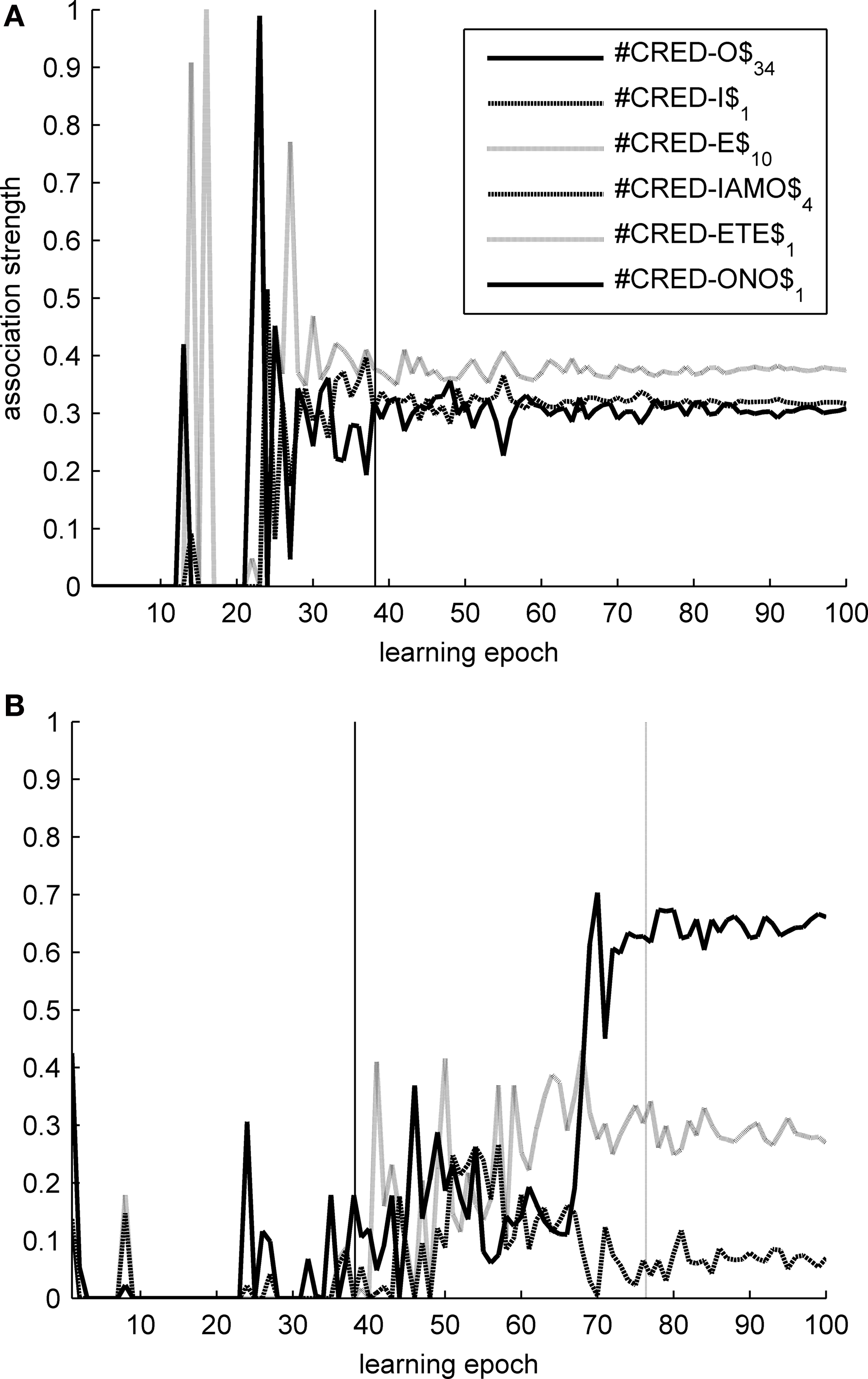
Figure 8. Transition probabilities over morpheme boundaries in CREDERE (‘believe’). (A) THSOM model; (B) T²HSOM model.

Experiment 2

In this experiment we tested the results of the two Bayesian models of gaze planning informally described in Section “Gaze planning in reading: a Bayesian ideal-observer perspective”. Like our T⁽²⁾HSOM based models, Algorithm 2 skips upcoming characters that are predicted reliably, but operates on complete word statistics and uses Bayes rules to update transition probabilities. Results are illustrated in Figure 9 , plotted against levels of confidence. Unsurprisingly, the performance of the system is better; in particular, with a threshold of 0.85, the system reaches 100% performance and predicts 54% of the characters. In addition, even with lower thresholds the correctness rate is high; this is due to the high prediction accuracy of the system. Therefore, the main lesson learned from this comparison is that the lexical representation network is still limited in its prediction ability, due to its local learning steps and its incrementality. We argue that this is the price we have to pay for modeling human behavior in a more realistic way. In fact, it is dubious that children can supposedly be engaged in a search for global optimization strategies in learning word reading.

FIGURE 9

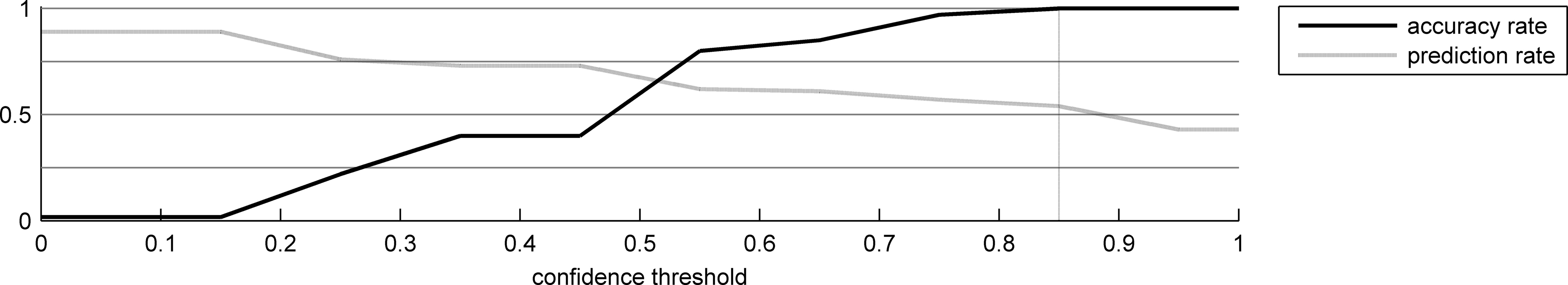
Figure 9. Results of the first algorithm having complete knowledge of the word statistics.

Algorithm 3 (also adopted in the design of Mr. Chips, Legge et al., 1997 , 2002 ) implements the Bayesian ideal-observer procedure described above ² . It calculates the expected information gain (i.e., difference between future and present entropy) of each possible character, and gazes the one with the highest information gain, independently of its position in the word. This is done again until the word is identified with 100% probability. This algorithm is optimal in Bayesian terms, with 2.42 gazes on average per word (from 2 to 4 gazes), corresponding to 30.1% read characters only, with a variance of 0.09. Recognition is 100% accurate. As expected, its performance is significantly better than the other algorithms presented here, at the cost of stronger assumptions (complete knowledge and indifference to the order of characters in words). The comparison sheds light on the difficulty of the task we designed. Indeed, our results show that the number of characters that could be skipped while preserving optimal performance is limited (consider however that in human reading and comprehension, predictions can be done at multiple levels, e.g., lexical, syntactic, semantic; see Pickering and Garrod, 2007 ).

Our experimental results, on the other hand, cannot be compared directly to human reading data. Not only human reading skills are considerably more sophisticated compared to our algorithm, but there are differences in the task requirements too. The human fovea can see about four or five characters around the fixation point with 100% acuity, and up to 10 times more with increasingly less acuity. On the contrary, we used a ‘fovea’ that only extracts 1 character per time. For this reason, it is reasonable that human saccades are on average 2–3 times longer (7–9 characters) than those obtained in our experiments (2–3 characters on average). In addition, the task we used was simplified compared to reading. For instance, humans ‘backtrack’ while reading (probably for correcting implausible interpretations). Our system was not allowed to backtrack, instead; wrong interpretations counted as errors.

Discussion and Concluding Remarks

We have implemented a computational model of eye movements in language reading that integrates two components: a lexical representation network and a gaze planner. The lexical representation network is a temporal self-organizing map, combining overlaying memory patterns with chains of first-order weighted Hebbian connections. From a cognitive perspective, this novel network architecture has two interesting implications.

A trained temporal map behaves like a first-order stochastic Markov chain, with inter-node connections building expectations about possible word forms on the basis of a global topological organization of already known forms. The model prompts a reappraisal of the traditional melee between one-route and dual-route models of morphology processing and learning, as it contextually represents lexical memory patterns and rule-like predictions. Furthermore, the architecture has something to say about the representation of serial order information in short-term and long-term memory structures.

Botvinick and Plaut (2006) contrast two general computational approaches to modeling short-term memory for serial order: weight-based models and activation-based models. In weight-based approaches (see, e.g., Grossberg, 1986 ; Houghton, 1990 ; Burgess and Hitch, 1992 , 1999 ; Houghton and Hartley, 1996 ; Hartley and Houghton, 1996 ; Henson, 1996 , 1998 ; Brown et al., 2000 ), serial encoding and recall depend on transient associative links between item and context representations, with associative links being established by changing the connection weights between processing units, upon presentation of a sequence to be recalled. Weight-based models may differ in the nature of the context representation they use, but they all agree that serial recall does not involve incremental learning. Thus, although they prove to be able to replicate a wide range of detailed behavioral findings about human subjects, they have so far failed to simulate effects of background long-term knowledge (e.g. Baddeley’s so-called bigram frequency effect, Baddeley, 1964 ).

Unlike weight-based approaches, activation-based memory mechanisms (such as recurrent neural networks and the T⁽²⁾HSOMs presented here) adjust weights gradually, over many learning trials, but performance of network recall is evaluated by holding weights constant and using sustained activation patterns. Botvinick and Plaut (2006) show that recurrent neural networks can account for long-term memory effects, while, at the same time, replicating several behavioral facts of human recall. However, this is achieved by accounting for short-term effects of serial recall on the basis of long-term memory effects. This is somewhat questionable. First, it makes short-term memory entirely depend on long-term memory mechanisms. In a developmental perspective, the causal relationship is in fact reversed (although reciprocal effects are also observed). For example, problems with short-term memory processing are known to cause delays in child vocabulary acquisition (Shallice and Vallar, 1990 ; Papagno et al., 1991 ; Service, 1992 to mention a few). As observed by Baddeley (2007) , children with higher short-term memory capacity are able to hold on to new words for longer, increasing the likelihood of long-term lexical learning. Finally, Botvinick and Plaut’s (2006) approach makes the paradoxical suggestion that human performance on immediate serial recall develops through direct practice on the task, rather than using the task to probe short-term memory capacities.

In T⁽²⁾HSOMs, the learning regime is unsupervised and memory effects are not based upon recall performance. Moreover, short-term memory and long-term memory work according to two different dynamics. Serial encoding in a temporal map requires sustained activation of BMUs and their one-way associative connections. Sustained activation chains of this kind are triggered upon presentation of an input sequence (see Building a Lexical Network with a T⁽²⁾HSOM above). We further argue here that, by smoothing the decay function over consecutive time steps, activation chains can also simulate effects of immediate serial recall. Serial learning, on the other hand, adjusts connection weights gradually, for them to keep track of the most frequently activated connections. Hence long-term entrenchment of one-way Hebbian connections is the result of repeated exposure to frequent time series of symbols. When long-term entrenchment sets in, it can affect immediate recall through anticipatory activation of the most frequently activated connection chains. In fact, this is the same mechanism we used in this paper to predict upcoming words. Temporal maps thus point to a profound continuity between word prediction, repetition and learning. Nonetheless they assume that short-term memory and long-term memory are based on different temporal dynamics, in line with neurobiological approaches (Pulvermüller, 2003 ) according to which long-term memory refers to consolidation of associative networks and short-term memory is (transient) activation of the same networks.

The gaze planner is motivated by a Bayesian ideal-observer perspective. It bears resemblances to Mr. Chips (Legge et al., 1997 , 2002 ), the first computational model based on an ideal-observer analysis, to the Bayesian reader (Norris, 2006 ), and to other Bayesian computational models of reading (Sprague and Ballard, 2003 ; Nelson and Cottrell, 2007 ). In all these systems, lexical predictions drive attention in such a way that uncertainty about environmental variables that are task relevant is reduced. This is done either by minimizing entropy, or by minimizing a combination of entropy and movement (i.e. saccade amplitude) costs. Compared to these models, our system adopts the simpler principle of gazing at the next character that cannot be reliably predicted, and works on top of learned (self-organized) lexical representations and lexical predictions.

Since a T⁽²⁾HSOM modifies its lexical representations and predictions during learning, our computational model allows us to analyze how gaze planning varies during reading, depending on the system’s lexical knowledge. In particular, it offers a framework to study the interrelated developmental trajectories of (lexical) knowledge acquisition and gaze planning during reading. To the best of our knowledge, there is no extensive empirical study of this aspect in reading, whereas relevant data exist related to other tasks. For instance, a recent study has investigated how visual strategies change when the subject learns a novel visuomotor task (Sailer et al., 2005 ). The authors found that better performance correlated with changes in gaze planning. At a first stage, hit rate was low and gaze was reactive, whereas in the second and third stages hit rate was higher and gaze become increasingly more predictive. In our experiments, we observed the same pattern of behavior, with the development of increasingly reliable predictions that were conducive to planning anticipatory strategies.

Surely, this developmental pattern is not confined to the domain of reading or vision. Several studies in other fields, such as motor development (von Hofsten, 2004 ), have revealed that the development of predictive abilities determines an increasing reliance on prospective behavior and is a necessary precondition for the rise of more and more complex cognitive abilities (for a discussion of this topic, see Pezzulo and Castelfranchi, 2007 ; Butz, 2008 ; Pezzulo, 2008 ).

Relevance of Our Study for (Developmental) Robotics

Our approach to reading as an active sensing process is based on representations and predictions that are increasingly refined through learning. This makes our model particular fit for developmental robotic implementations. Through our methodology, lexical representations can be acquired and further exploited to engage in both linguistic and extra-linguistic tasks in human-robot, or robot-robot scenarios. In addition, the model can be extended to study the acquisition of referential capabilities in robots. This could be done, for instance, by coupling many T⁽²⁾HSOMs, one for each domain (visuomotor, linguistic, etc.), for acquiring a combined lexical representation of a word such as ball, a visual representation of balls, and a set of actions to be performed on balls, so that the robot can use language to refer to objects and actions in the world, along the lines of recent computational studies that combine linguistic and sensorimotor processes (Cangelosi and Harnad, 2001 ; Roy, 2005 ; Sugita and Tani, 2005 ; Wermter et al., 2005 ).

It is worth noting that our active sensing methodology is applicable outside the linguistic domain. In general, the problem of how, during development, task representations are acquired and determine increasingly sophisticated active sensing strategies, is characteristic of any form of sensorimotor learning. In addition, as pointed out above, there is substantial evidence that anticipatory processes drive visual strategies in many visuomotor tasks (Hayhoe and Ballard, 2005 ). Therefore, by using T⁽²⁾HSOMs to encode sensorimotor rather than linguistic predictions, our methodology could be adopted for the visual guidance of actions, with attention going where (task) relevant information is expected to be.

Future Work

We rapidly mention here two aspects of our model that are particularly promising for future work. The predictive nature of our model makes room for novelty detection (Bishop, 1994 ), i.e. identification of novel data from on the basis of marginal density. In particular, the model could classify words or sentences as novel. In turn, novelty detection is a fundamental precondition for active learning based on adaptive curiosity, which consists in focusing learning on novel but still predictable parts of the data, for which the system can actually improve its predictions (Schmidhuber, 1991 ). In our current model, the two sub-tasks of lexical acquisition and word recognition are carried out independently. However, they could be combined so that the gaze planning mechanism is active during learning and the novelty detection mechanism can affect learning lexical representations in the T⁽²⁾HSOM. In the first learning stages, when lexical representations in the T⁽²⁾HSOMs are not fully developed and reliable, most input text contributes novel information, with few characters being skipped and lexical representations being frequently revised. When lexical representations in the T⁽²⁾HSOMs get more deeply entrenched and dependable, novelties become more rare, more characters are skipped, and lexical representations get revised only occasionally.

Another possible extension of our model is using a cascaded asynchronous T⁽²⁾HSOM architecture, with higher-level maps sampling the activation state of lower-level maps at increasingly larger time intervals. In this architecture, short-range (i.e., phonological and morphological) serial correlations are captured through low-level maps, and long-range serial correlations (i.e., word sequences) are represented on top-level maps. Although a single T⁽²⁾HSOM could in principle capture correlations at all levels (size allowing), with the benefit of the hindsight (Calderone et al., 2007 ) we conjecture that cascaded architectures of this type can encode correlations more efficiently, avoiding information overload/interference and effectively simulating the interaction of short-term and long-term memory effects in human serial recall.

Appendix

The T⁽²⁾HSOM Model

Short-term dynamics: activation and filtering

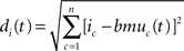
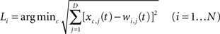
In the topological processing phase, activation of each node is a function of the Euclidean distance in the input space between its weight vector and the input vector. The resulting topological activation of the i-th node at time t is:

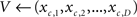
where D is the number of components of the input vector X(t) = [x₁(t),…,x_D(t)], and w_i,j(t) is the synaptic weight of the topological connection between the i-th node and the j-th input component.

In the temporal processing phase, activation of each neuron is a function of the correlation between its temporal synaptic connections and the overall activation state at the previous time step. The resulting temporal activation of the i-th node at time t is:

where N is the number of node of the map, Y(t−1) = [y₁(t−1),…, y_N(t−1)] is the output of the T⁽²⁾HSOM at the previous time step, and m_i,h(t) is the synaptic weight of the temporal connection from the h-th pre-synaptic neuron to the i-th post-synaptic neuron.

The resulting two activation values are summed up, so that the resulting activation value of the i-th neuron at time t is:

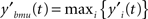
The filtering module identifies BMU at time t by looking for the maximum activation level:

The output is subsequently normalized to ensure the network stability over time:

Long-term dynamics: learning

In T⁽²⁾HSOM learning consists in topological and temporal co-organization.

Topological learning. In classical SOMs, this effect is taken into account by a neighborhood function centered around BMU. Nodes that lie close to BMU on the map will be strengthened as a function of BMU’s neighborhood. The distance between BMU and the i-th node on the map is calculated through the following Euclidean metrics:

where n is 2 when the map is two-dimensional. The topological neighborhood function of the i-th neuron is defined as a Gaussian function with a cut-off threshold:

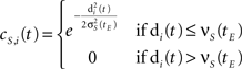
where σ_S(t_E) is the topological neighborhood shape coefficient at epoch time t_E, and ν_S(t_E) is the topological neighborhood cut-off coefficient at epoch time t_E.

The synaptic weight of the j-th topological connection of the i-th node at time t + 1 and epoch t_E, is finally modified as follows:

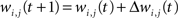
where α_S(t_E) is the topological learning rate at t_E.

Temporal learning

On the basis of BMU at time t−1 and BMU at time t, three learning steps are taken:

• temporal connections from BMU at time t−1 (the j-th neuron) to the neighborhood of BMU at time t (the i-th neurons) are strengthened:

• temporal connections from all neurons except BMU at time t−1 (the j-th neurons) to the neighborhood of BMU at time t (the i-th neurons) are depressed as well:

• temporal connections from BMU at time t−1 (the j-th neuron) to outside the neighborhood of BMU at time t (the i-th neurons) are depressed as well:

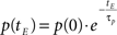
Learning decay. As an epoch ends, an exponential decay process applies to each learning parameter so that the generic parameter p at t_E is calculated according to the following equation:

A complete list of the learning parameters is shown below:

• α_S: learning rate of the topological learning process

• σ_S: shape parameter of the neighborhood Gaussian function for the topological learning process

• ν_S: cut-off distance of the neighborhood Gaussian function for the topological learning process

• α_T: learning rate of the temporal learning process

• σ_T: shape parameter of the neighborhood Gaussian function for the temporal learning process

• ν_T: cut-off distance of the neighborhood Gaussian function for the temporal learning process

• β_T: offset of the Hebbian rule within the temporal learning process

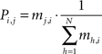
Post processing. At a given epoch t_E, the transition matrix is extracted from the temporal connection weights m_i,j(t_E), so that P_i,j(t_E) is the probability to have a transition from the i-th node to the j-th node of the network (i.e., the j-th node will be the BMU at time t + 1, given the i-th node is the BMU at time t):

At the same time the labeling procedure is applied. A label L_i (i.e., an input symbol) is assigned to each node, so that the grapheme-base coding of the c-th symbol matches the i-th node’s space vector best:

Parameter configuration

The experiments shown in the present work were performed using the following parameter configuration:

• 25 × 25 map nodes

• 20 elements in the input vector (grapheme-based orthographic character coding)

• 100 learning epochs

• learning rates starting from maximum value (i.e. 1.0), exponentially decaying over epochs with a time-constant equal to 25 epochs

• shape parameters starting from a value so that the Gaussian function has a gain equal to 30% at the maximum cut-off distance, with no decay over epochs

• spatial cut-off distance starting from the maximum distance between two nodes in the map, exponentially decaying over epochs with a time-constant equal to 12.5 epochs

• temporal cut-off distance starting from the maximum distance between two nodes in the map, exponentially decaying over epochs with a time-constant equal to 25 epochs

• offset of the Hebbian rule within the temporal learning process starting from 0.01), exponentially decaying over epochs with a time-constant equal to 25 epochs

The THSOM version of the model was tested by using ν_T = 0 and σ_T = ∞.

Algorithm 1

The performance of the T⁽²⁾HSOM model is evaluated in terms of accuracy and prediction rate during the execution of the reading task of single words. During this stage the learning algorithm of the model is turned off. The algorithm takes into account all the words contained in the dictionary, and all the symbols contained in each word. With the aim to identify the optimal confidence threshold θ, the corresponding domain (0 ≤ θ ≤ 1) is sampled in 100 steps and the performance rates are evaluated at each step.

For each word in dictionary, assuming s_i,j represents the j-th symbol of the i-th word, the algorithm starts from the left-most symbol (i.e. j ← 1) and performs the following steps:

(1) the j-th symbol of the i-th input word is collected:

c ← s_i,j

(2) the symbol c is queued in the output word:

s’_i,j ← c

(3) a look-up table provides the D-element vector V representing the grapheme-based coding belonging to the symbol c:

(4) the input vector V is propagated into the model and, as a result, a new BMU gets activated:

k ← BMU

(5) the algorithm looks for the highest transition probability among all the outgoing (post-synaptic) connections from the k-th node of the network:

(6) if P_k,q is above the confidence threshold θ, then the next symbol can be directly obtained (i.e., predicted) as the label of the q-th node of the network:

c ← L_q

(7) if this the case, the algorithm returns to step (2). Otherwise, the next symbol must be collected (i.e., read) from the input word, returning to step (1). In both cases, the algorithm continues with the next symbol (j ← j + 1) of the current word. If the end-of-word is reached, the next word is processed (j ← 1; i ← i + 1) until the end-of-dictionary is reached.

During the previous steps, the algorithm evaluates the following scores:

• for each word, the ratio between the number of predicted symbols and the number of total symbols of the word (the start-of-word symbol is excluded)

• the prediction rate, which is obtained averaging the above mentioned ratio over all the words

• for each word, the Boolean comparison between the input word s_i and the output word s’_i

• the accuracy rate, which is obtained as the ratio between the number of words predicted correctly (i.e., there is no difference between the input and output word) and the total number of words in the dictionary

Algorithm 2

The first algorithm described in Section “Experiment 2” operates with complete knowledge (of the order/probability of the characters in the words) and skips predictable characters. Given the current belief state [i.e. a vector b_t(w_i) that describes the probability that the already gazed characters belong to one of the words in the dictionary (w_i)] and the current position a_t, the algorithm selects the character o_m that has the maximum probability P_m to be the next character (at position a_{t + 1}) in the word being read.

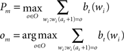
If the maximum probability is more than a threshold θ, the algorithm assumes that o_m has been read (or can be skipped), otherwise it reads the character at position a_t + 1. Then, it updates the belief state b_{t+ 1}(w_i) and sets the new initial position (a_{t + 1}←a_t + 1). This procedure continues until the end of the word.

Algorithm 3

The second algorithm described in Section “Experiment 2” uses the probability distribution of the words in the dictionary, given the characters already read and the priors (of which it has complete knowledge). The aim of the algorithm is selecting the action (i.e., gaze position) that results in an observation (i.e. a read character), which, in turn, minimizes (on average) the expected entropy, or the entropy of the resulting probability distribution of the words in the entire dictionary, given the current belief state (i.e. word probability) ³ . Note that this approach is myopic, since it minimizes entropy of the next step only (not of the entire sequence of gazes). In general, there is no guarantee that a sequence of myopic actions achieves the same decrease of entropy as an optimal non-myopic sequence.

The initial probability of word w_i is b₀(w_i), and corresponds to the frequency of the word in the corpus. The vector b₀ is the belief state of the agent. The following formulas describes how beliefs (b_{t + 1}) are updated based on (i) the previous belief state (b_t), (ii) the new observation (o_{t + 1}), and (iii) the executed action (a_t).

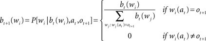
When the algorithm gets the character o_{t + 1} at position a_t, the probability distribution of words is updated as follows: (i) it becomes zero for all words that have a different character in that position, (ii) for all the other words, the previous probability is divided by the sum of the previous probability of all the words that have the character in the right position. Expected entropy (EH), given the current belief and the position gazed (a_t), is calculated as indicated by the next formula:

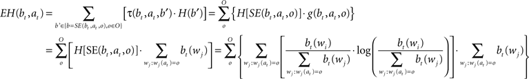
Function τ(b_t,a_t,b’) gives the probability of obtaining the belief state b’ given current belief state b_t and gazing at position a_t, while H(b’) is the entropy of the belief state b’ corresponding to the distribution of probability over the dictionary {w_i}. SE(b_t,a_t,o) is the belief state that, starting from belief state b_t is obtained after the execution of action a_t resulting in the observation o. g(b_t,a_t,o) is the probability of getting observation o by executing action a_t in belief state b_t (i.e., the sum of probabilities of all words matching all read characters and with character o at position a_t).

It is worth noting that the use of this computational approach in realistic reading tasks is hindered by its computational cost (which grows quadratically with the length of the word/text to be read), and by its huge demands in terms of knowledge (it implicitly assumes that all the possible words/texts are already known, and the current task consist in recognizing which word/text one is currently reading). For text reading, a more feasible computational approach could be adopted that uses this method at two or more levels in parallel, for instance at the level of single words and at the same time at the level of whole sentences (using words and not characters as observations, and changing the priors on words). Another limit of this algorithm is that it doesn’t model noise in action (e.g., one can believe to be reading the 5th character, but actually read the 6th) and observation (e.g., one can mistake an “l” for a “i”). Modeling noise would result in more complex algorithms like those for planning in POMDP.

Conflict of Interest Statement

The authors declare that the research was conducted in the absence of any commercial or financial relationships that could be construed as a potential conflict of interest.

Acknowledgments

The research leading to these results has received funding from the European’s Community Seventh Framework Programme under grant agreement no FP7-231453 (HUMANOBS, Humanoids That Learn Socio-Communicative Skills Through Observation).

Footnotes

1. ^ Hereafter, we shall use the acronym T⁽²⁾HSOM when we want to say things that apply to both temporal variants of SOMs illustrated in the present section.
2. ^ The algorithms we present here were selected as benchmarks for their simplicity, and many others could be adopted that implement similar ideal-observer strategy, with the addition of extra constraints. First, note that the strategy implemented here is myopic, in that the information gain is calculated only for the next saccade, and not (cumulatively) for whole sequences of saccades. Although the latter strategy is optimal in principle, it is however extremely demanding in computational terms. In addition, one could take into consideration extra factors, such as (motor) costs for the saccades, so that longer saccades are dispreferred, or costs for errors in the word recognition, so that system must find the minimum cumulative loss instead of simply minimizing the number of saccades. Note also that alternative Bayesian strategies have been proposed such as the “optimal ambiguity resolution” procedure of (Chater et al., 1998 ), which introduces a bias to choose interpretations which make specific predictions, and which might be falsified quickly.
3. ^ The notation used, (action a, belief b and observation o) is typical of POMDP, which is a formalization of the problem of choosing sequences of actions under uncertainty in order to achieve an optimal total reward.

References

Altmann, G. T. M., and Kamide, Y. (1999). Incremental interpretation at verbs: restricting the domain of subsequent reference. Cognition 73, 247–264.

Pubmed Abstract | Pubmed Full Text | CrossRef Full Text

Baayen, H. (2007). “Storage and computation in the mental lexicon,” In The Mental Lexicon: Core Perspectives, eds G. Jarema and G. Libben (Amsterdam: Elsevier), 81–104.

Baddeley, A. D. (1964). Immediate memory and the “perception” of letter sequences. Q. J. Exp. Psychol. 16, 364–367.

CrossRef Full Text

Baddeley, A. D. (2007). Working Memory, Thought, and Action. Oxford: Oxford University Press.

Ballard, D. H. (1991). Animate vision. Artif. Intell. 48, 1–27.

CrossRef Full Text

Ballard, D. H., Hayhoe, M. M., and Pelz, J. B. (1995). Memory representations in natural tasks. J. Cogn. Neurosci. 7, 66–80.

CrossRef Full Text

Bishop, C. M. (1994). Novelty detection and neural network validation. IEE Proc., Vis. Image Process 141, 217–222.

CrossRef Full Text

Botvinick, M. M., and Plaut, D. C. (2006). Short-term memory for serial order: a recurrent neural network model. Psychol. Rev. 113, 201–233.

Pubmed Abstract | Pubmed Full Text | CrossRef Full Text

Brown, G., Preece, T., and Hulme, C. (2000). Oscillator-based memory for serial order. Psychol. Rev. 107, 127–181.

Pubmed Abstract | Pubmed Full Text | CrossRef Full Text

Burani, C., Marcolini, S., De Luca, M., and Zoccolotti, P. (2008). Morpheme-based reading aloud: evidence from dyslexic and skilled Italian readers. Cognition 108, 1, 243–262.

CrossRef Full Text

Burgess, N., and Hitch, G. J. (1992). Toward a network model of the articulatory loop. J. Mem. Lang. 21, 429–460.

CrossRef Full Text

Burgess, N., and Hitch, G. J. (1999). Memory for serial order: a network model of the phonological loop and its timing. Psychol. Rev. 106, 551–581.

CrossRef Full Text

Burzio, L. (2004). “Paradigmatic and syntagmatic relations in Italian verbal inflection,” in Contemporary Approaches to Romance Linguistics, eds J. Auger, J. C. Clements and B. Vance (Amsterdam: John Benjamins), 17–44.

Butz, M. V. (2008). How and why the brain lays the foundations for a conscious self. Constructivist Found. 4, 1–42.

Calderone, B., Herreros, I., and Pirrelli, V. (2007). Learning Inflection: the importance of starting big. Lingue e Linguaggio 2, 175–200.

Cangelosi, A., and Harnad, S. (2001). The adaptive advantage of symbolic theft over sensorimotor toil: grounding language in perceptual categories. Evol. Commun. 4, 117–142.

CrossRef Full Text

Chater, N., Crocker, M. J., and Pickering, M. J. (1998). “The rational analysis of inquiry: the case of parsing” in Rational Models of Cognition, eds M. Oaksford and N. Chater (Oxford: Oxford University Press), 441–469.

DeLong, K. A., Urbach, T. P., and Kutas, M. (2005). Probabilistic word pre-activation during language comprehension inferred from electrical brain activity. Nat. Neurosci. 8, 1117–1121.

Pubmed Abstract | Pubmed Full Text | CrossRef Full Text

Ehrlich, S. E., and Rayner, K. (1981). Contextual effects on word perception and eye movements during reading. J. Verbal Learn. Verbal Behav. 20, 641–655.

CrossRef Full Text

Engbert, R., and Krügel, A. (2010). Readers use Bayesian estimation for eye-movement control. Psychol. Sci. 21, 366–371.

Pubmed Abstract | Pubmed Full Text | CrossRef Full Text

Federmeier, K. D. (2007). Thinking ahead: the role and roots of prediction in language comprehension. Psychophysiology 44, 491–505.

Pubmed Abstract | Pubmed Full Text | CrossRef Full Text

Geisler, W. S. (2003). “Ideal observer analysis,” in The Visual Neurosciences, eds L. Chalupa and J. Werner (Boston: MIT press) 825–837.

Grossberg, S. (1986). “The adaptive self-organization of serial order in behavior: speech, language, and motor control,” in Pattern Recognition by Humans and Machines Vol. 1: Speech Perception, eds E. C. Schwab and H. C. Nusbaum. (New York: Academic Press), 187–294.

Hartley, T., and Houghton, G. (1996). A linguistically constrained model of short-term memory for nonwords. J. Mem. Lang. 35, 1–31.

CrossRef Full Text

Hayhoe, M., and Ballard, D. H. (2005). Eye movements in natural behavior. Trends Cogn. Sci. (Regul. Ed.) 9, 188–193.

Pubmed Abstract | Pubmed Full Text

Hebb, D. O. (1949). The Organisation of Behaviour. New York: Wiley.

Henson, R. N. A. (1996). Short-term memory for serial order. Unpublished doctoral dissertation, MRC Applied Psychology Unit. Cambridge: University of Cambridge.

Henson, R. N. A. (1998). Short-term memory for serial order: The start-end model. Cogn. Psychol. 36, 73–137.

Pubmed Abstract | Pubmed Full Text | CrossRef Full Text

Houghton, G. (1990). “The problem of serial order: a neural network model of sequence learning and recall,” in Current Research in Natural Language Generation, eds R. Dale, C. Nellish and M. Zock (San Diego: Academic Press), 287–318.

Pubmed Abstract | Pubmed Full Text

Houghton, G., and Hartley, T. (1996). Parallel models of serial behaviour: Lashley revisited. Psyche 2, 2–25.

Howard, R. A. (1966). Information value theory. IEEE Trans. Syst. Sci. Cybern. 2, 22–26.

CrossRef Full Text

Jenkins, W., Merzenich, M. M., and Ochs, M. (1984). Behaviorally controlled differential use of restricted hand surfaces induces changes in the cortical representation of the hand in area 3b of adult owl monkeys. Abstr. - Soc. Neurosci. 10, 665.

Johansson, R. S., Westling, G., Bäckström, A., and Flanagan, J. R. (2001). Eye-hand coordination in object manipulation. J. Neurosci. 21, 6917–6932.

Pubmed Abstract | Pubmed Full Text

Kaas, J. H., Merzenich, M. M., and Killackey, H. (1983). The reorganization of somatosensory cortex following peripheral nerve damage in adult and developing mammals. Annu. Rev. Neurosci. 6, 325–356.

Pubmed Abstract | Pubmed Full Text | CrossRef Full Text

Kohonen, T. (2001). Self-Organizing Maps. Heidelberg: Springer-Verlag.

Koutnik, J. (2007). “Inductive modelling of temporal sequences by means of self-organization,” in Proceeding of International Workshop on Inductive Modelling (IWIM 2007), Prague, 269–277.

Land, M. F. (2006). Eye movements and the control of actions in everyday life. Prog Retin Eye Res 25, 296–324.

Pubmed Abstract | Pubmed Full Text | CrossRef Full Text

Legge, G. E., Hooven, T. A., Klitz, T. S., Mansfield, J. S., and Tjan, B. S. (2002). Mr. Chips 2002: New insights from an ideal-observer model of reading. Vision Res. 42, 2219–2234.

Pubmed Abstract | Pubmed Full Text | CrossRef Full Text

Legge, G. E., Klitz, T. S., and Tjan, B. S. (1997). Mr. Chips: An ideal-observer model of reading. Psychol. Rev. 104, 524–553.

Pubmed Abstract | Pubmed Full Text | CrossRef Full Text

Libben, G. (2006). “Why studying compound processing? An overview of the issues,” in The Representation and Processing of Compound Words, eds G. Libben and G. Jarema (Oxford: Oxford University Press), 1–22.

MacWhinney, B. (2000). The CHILDES Project: Tools for Analyzing Talk, volume 2: The Database. Hillsdale, NJ: Lawrence Erlbaum.

McClelland, J., and Patterson, K. (2002). Rules or connections in past-tense inflections: what does the evidence rule out? Trends Cogn. Sci. 6, 465–472.

Pubmed Abstract | Pubmed Full Text | CrossRef Full Text

Nelson, J. D., and Cottrell, G. W. (2007). A probabilistic model of eye movements in concept formation. Neurocomputing 70, 2256–2272.

CrossRef Full Text

Norris, D. (2006). The Bayesian reader: explaining word recognition as an optimal Bayesian decision process. Psychol. Rev. 113, 327–357.

Pubmed Abstract | Pubmed Full Text | CrossRef Full Text

O’Regan, J., and Nöe, A. (2001). A sensorimotor account of vision and visual consciousness. Behav. Brain Sci. 24, 883–917.

Papagno, C., Valentine, T., and Baddeley, A. (1991). Phonological short-term memory and foreign-language learning. J. Mem. Lang. 30, 331–347.

CrossRef Full Text

Penfield, W., and Rasmussen, T. (1950). The Cerebral Cortex of Man. New York: Macmillan.

Penfield, W., and Roberts, L. (1959). Speech and Brain Mechanisms. Princeton: Princeton University Press.

Pezzulo, G. (2008). Coordinating with the future: the anticipatory nature of representation. Minds Machine 18, 179–225.

CrossRef Full Text

Pezzulo, G., and Castelfranchi, C. (2007). The symbol detachment problem. Cogn. Process. 8, 115–131.

Pubmed Abstract | Pubmed Full Text | CrossRef Full Text

Pickering, M. J., and Garrod, S. (2007). Do people use language production to make predictions during comprehension? Trends Cogn. Sci. (Regul. Ed.) 11, 105–110.

Pubmed Abstract | Pubmed Full Text

Pinker, S., and Prince, A. (1988). On language and connectionism: analysis of a parallel distributed processing model of language acquisition. Cognition 29, 195–247.

Pinker, S., and Ullman, M. T. (2002). The past and future of the past tense. Trends Cogn. Sci. 6, 456–463.

Pubmed Abstract | Pubmed Full Text | CrossRef Full Text

Pirrelli, V. (2007). Psychocomputational issues in morphology learning and processing: an ouverture. Lingue Linguaggio 2, 131–138.

Pirrelli, V., Ferro, M., and Calderone, B. (in press). “Learning paradigms in time and space. Computational evidence from Romance languages,” in Morphological Autonomy: Perspectives from Romance Inflectional Morphology, eds M. Goldbach, M. O. Hinzelin, M. Maiden and J. C. Smith (Oxford: Oxford University Press).

Post, B., Marslen-Wilson, W., Randall, B., and Tyler, L. K. (2008). The processing of English regular inflections: Phonological cues to morphological structure. Cognition 109, 1–17.

Pubmed Abstract | Pubmed Full Text | CrossRef Full Text

Prasada, S., and Pinker, S. (1993). Generalization of regular and irregular morphological patterns. Lang. Cogn. Process. 8, 1–56.

CrossRef Full Text

Pulvermüller, F. (2003). Sequence detectors as a basis of grammar in the brain. Theory Biosci. 122, 87–103.

Rayner, K. (2009). Eye movements and attention in reading, scene perception, and visual search. Q. J. Exp. Psychol. 62, 1457–1506.

CrossRef Full Text

Rayner, K., and Well, A. D. (1996). Effects of contextual constraint on eye movements in reading: A further examination. Psychon. Bull. Rev. 3, 504–509.

Roy, D. (2005). Semiotic schemas: a framework for grounding language in action and perception. Artif. Intell, 167, 170–205.

CrossRef Full Text

Sailer, U., Flanagan, J. R., and Johansson, R. S. (2005). Eye-hand coordination during learning of a novel visuomotor task. J. Neurosci. 25, 8833–8842.

Pubmed Abstract | Pubmed Full Text | CrossRef Full Text

Schmidhuber, J. (1991). Adaptive Confidence and Adaptive Curiosity. Institut für Informatik, Technische Universitat, Munchen.

Service, L. (1992). Phonology, working memory and foreign-language learning. Q. J. Exp. Psychol. A. 45, 21–50.

Pubmed Abstract | Pubmed Full Text

Shallice, T., and Vallar, G. (1990). “The impairment of auditory-verbal short-term storage,” in Neuropsychological Impairments of Short-Term Memory, eds G. Vallar and T. Shallice (Cambridge: Cambridge University Press), 121–141.

Sprague, N., and Ballard, D. H. (2003). “Eye movements for reward maximization,” in Proceedings of Advances in Neural Information Processing Systems 16 (NIPS’03), eds S. Thrun, L. Saul and B. Schölkopf (Cambridge: MIT Press), 1467–1474.

Sugita, Y., and Tani, J. (2005). Learning semantic combinatoriality from the interaction between linguistic and behavioral processes. Adapt. Behav. 13, 33–52.

CrossRef Full Text

Triesch, J. J., Ballard, D. H., Hayhoe, M., and Sullivan, B. (2003). What you see is what you need. J. Vis. 3, 86–94.

Pubmed Abstract | Pubmed Full Text | CrossRef Full Text

Ullman, M. T. (2004). Contributions of memory circuits to language: the declarative/procedural model. Cognition 92, 231–270.

Pubmed Abstract | Pubmed Full Text | CrossRef Full Text

von Hofsten, C. (2004). An action perspective on motor development. Trends Cogn. Sci. 8, 266–272.

Pubmed Abstract | Pubmed Full Text | CrossRef Full Text

Wermter, S., Weber, C., and Elshaw, M. (2005). “Associative neural models for biomimetic multi-modal learning in a mirror neuron-based robot,” in Modeling Language, Cognition and Action, eds A. Cangelosi, G. Bugmann and R. Borisyuk (Singapore: World Scientific), 31–46.

Westermann, G., and Plunkett, K. (2007). Connectionist models of inflection processing. Lingue Linguaggio 2, 291–311.

Yarbus, A. (1967). Eye Movements and Vision. New York: Plenum Press.