Impedance Control for Robotic Rehabilitation: A Robust Markovian Approach

1. Introduction

Physical therapy represents a well-accepted procedure for improvements in the recovery of human motor function and promotion of higher performance in Activities of Daily Life (ADLs) (Krebs et al., 2008). Mainly when people have been affected by injuries such as stroke (Hatano, 1976) and Multiple Sclerosis (MS) (Cattaneo et al., 2002). Robotic-assisted therapy is a promising field for the development of rehabilitation tasks. Among the advantages offered by robotic devices are uniformity in the repetition of long-time routines, reliable records of measured variables, and motivation for the patient's participation using interactive environments like serious games (Lum et al., 2002; Chang and Kim, 2013; Gonçalves et al., 2014). However, the fact that these robots interact with humans during therapeutic movement, they require a high degree of security and reliability. Therefore, rehabilitation robots should identify activities performed by the patient to reach only pre-defined training objectives, whose principle is known as Assist-as-Needed Paradigm (Radomski and Trombly, 2013).

Impedance control has been used in the implementation of this kind of paradigm in rehabilitation robotic systems. It was initially proposed for manipulator robots to obtain a safe physical interaction with the environment (Hogan, 1985). Such a controller aims at establishing a dynamic relationship between the force and velocity of an actuator. Series elastic actuators (SEA) provide a simple and efficient solution for the implementation of impedance controllers (Calanca et al., 2016). However, the impedance control of SEAs requires an explicit force control loop whose performance is sensitive to uncertainties and time-varying human dynamics.

Colgate and Hogan (1988, 1989) addressed the problem of interaction control and analyzed the energy exchange between a robotic system and its environment, defined as passive. They also determined stability criteria for a coupled system. Some years later this analysis was brought into the context of human-robot interaction considering three new issues: (1) Human dynamics is now the environment; (2) This dynamics can exhibit passive and active behaviors; and, (3) The stability criterion has been reformulated as complementary stability (Buerger and Hogan, 2007). Such new concepts emphasize the way the human dynamics is taken into account. For example, Vallery et al. (2008) analyzed limits of coupled stability and performance of an SEA actuator for rehabilitation applications considering the human dynamics a spring and damping system. Kong et al. (2009) analyzed those limits considering the human dynamics only as a mass (inertia). In Oh and Kong (2017), the human dynamics was considered as stiffness, damping, and inertia. Li et al. (2017) proposed an adaptive control scheme for SEA-driven robots which consider two operation modes in the adaptation process, namely robot-in-charge and human-in-charge. Similar approaches were proposed in Yu et al. (2015) and Pan et al. (2017), however, the authors did not take into account the fact the human-robot system can be modeled by different operation modes related to abrupt changes in the dynamic behavior.

This paper reports on the implementation of an impedance controller in a robotic platform for ankle rehabilitation based on a Markovian approach. The platform uses an SEA and enables plantarflexion and dorsiflexion movements. The following three operation modes that may occur in the robot-human interaction were defined: (1) fixed mode, in which the platform is mechanically fixed; (2) resistive mode, in which the user makes efforts against the platform movement; and (3) passive mode, in which the user does not make any effort against the platform movement. Such operation modes are modeled as states of a Markov chain. Based on this modeling, a recursive robust regulator for discrete Markov jump linear systems (RR-DMJLS) proposed in Cerri and Terra (2017) is designed to regulate the force control. It guarantees mean square stability and optimal performance for this class of stochastic system (Jutinico et al., 2017). In order to check the effectiveness of the approach, we performed a comparative study with a standard ${{H}}_{\infty }$ force controller proposed in Pérez-Ibarra et al. (2017) which is designed based only on the higher-impedance operation mode (fixed). Although this control approach provides robust stability for the whole system, including all operation modes, its performance was outperformed by RR-DMJLS. We present actual results based on force- and impedance-control for both controllers.

The paper is organized as follows: Section 2 introduces the SEA-based robotic platform and its respective dynamic model; Section 3 describes the design of the robust controllers; Section 4 reports experimental results of a comparative study between the controllers; finally, Section 5 provides the conclusions and some final remarks for future work.

2. System Description and Modeling

The SEA-based Robotic Platform for Ankle Rehabilitation (SRPAR), Figure 1, is a device for robot-assisted training. It works under two conditions: guidance of a physiotherapist during pre-established dorsi/plantarflexion movements of the ankle and active participation of the patient by using serious games. Both conditions benefit individuals who have suffered a stroke. Also, the platform is a tool to evaluate the ankle force and range of movement (Gonçalves et al., 2013).

FIGURE 1

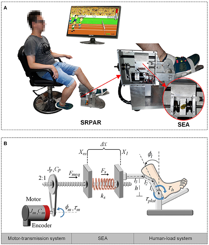
Figure 1. SEA-based Robotic Platform for Ankle Rehabilitation (SRPAR). (A) Platform (Gonçalves et al., 2014). (B) Squematic model.

The platform uses a DC motor (Maxon Motor RE 40, graphite brushes, 150 Watt DC motor) linked to a ballscrew through a belt and pulleys with 2:1 reduction ratio. A recirculating ballscrew nut converts the rotational motion of the screw in a linear motion. A pair of steel springs is attached to the nut and to a movable piece. When the motor is driven, the nut moves forward or backward compressing the springs. The movable part is connected to a kinematic chain which converts linear force into torque which is transferred to the user. We estimate the nut's position by measuring the motor rotation with a magneto-resistant incremental encoder. Finally, we estimate the spring force by measuring the spring deformation. A logarithmic sliding potentiometer is attached to the movable piece located between the springs. The potentiometer's cursor moves along with the piece generating a voltage proportional to the spring deformation.

2.1. Transfer Function Model

In order to describe the dynamic behavior of the system, we define three sub-systems in the SRPAR: motor-transmission system, series elastic element, and human-load system (Figure 1B). A set of assumptions is made to simplify the dynamic modeling, resulting in a linear model for the SRPAR. Although these simplifications can result in a limited model, mainly due to the presence of nonlinearities, the use of robust controllers to deal with uncertain parameters can improve the performance of the system.

Concerning the motor-transmission sub-system, although some studies deal with only the effect of the inertia in the motor model (Vallery et al., 2008; Calanca et al., 2014), in this paper we also consider the influence of the motor damping. The effects of the inertia and damping parameters of the pulley and ballscrew are also considered as in Yu et al. (2013) and dos Santos et al. (2015). In addition, the nonlinear effects of friction, backslash, and efficiency losses in the motor-transmission system are minimized by controlling the motor velocity instead of directly controlling the motor torque or current, as discussed in Wyeth (2006).

Regarding the series elastic configuration, in Petit et al. (2015) is presented a generic model for robotic systems with variable stiffness. They describe the output torque of the actuator by a nonlinear function that depends on the joint deflection and mechanical stiffness variation of the springs. In this paper, the springs are modeled as constant stiffness and operate in a linear region. Since the human limb is attached to the four-bar mechanism of the SRPAR, rotation of the ankle is transformed into a linear movement in the same direction of the spring force by a nonlinear Jacobian. However, due to a small range of allowed movements related to mechanical constraints of the SRPAR, this transformation is approximated by a linear relationship (see Equation 6). The gravity effects on the human foot are also neglected since the distance between the foots center of gravity and the rotation axis of the platform is small.

Different approaches have been proposed to model the dynamics of the human-load sub-system. For example, Tagliamonte and Accoto (2014) used a set of second-order plants to represent human dynamics in order to implement an impedance controller where passivity concepts are explored. In Lee et al. (2016), similar second-order models are used to measure the ankle mechanical impedance in a unified way. In this paper, we model the human dynamics as a set of second-order linear plants subject to parameter uncertainties.

In the following, we present a transfer function between the commanded motor velocity ${\omega }_m^d$ and the spring force F_s.

2.1.1. Dynamics of the Motor-Transmission System

Motor-transmission can be modeled as a second-order control system,

$\begin{array}{cc}{M}_{meq}{\ddot{X}}_w+B_{meq}{\dot{X}}_w=F_{meq}-F_s,& \left(1\right)\end{array}$

where X_w denotes the displacement of ball screw nut, M_meq and B_meq are respectively the equivalent inertia and damping of the system as defined in Equation (2), and F_meq is the output force as defined in Equation (3),

$\begin{array}{cc}{M}_{meq}=M_t+{\rho }^2(J_p+N_p^2{J}_m)\text{and}{B}_{meq}=B_t+{\rho }^2(C_p+N_p^2{C}_m).& \left(2\right)\end{array}$

$\begin{array}{cc}{F}_{meq}=\rho N_p{K}_t{i}_m=\rho N_p{K}_t\left((K_p+\frac{K_i}{s})({\omega }_m^d-{\omega }_m)\right).& \left(3\right)\end{array}$

In Equations (2) and (3), M_t and B_t are the mass and damping of the ball screw nut, J and C are torsional inertia and damping where subscripts _m and _p stand for motor and pulley, respectively. N_p is the pulley ratio, $\rho =\frac{2\pi }{l}$ is a rotational-to-linear factor where l is the ball screw lead. K_t is the motor constant, i_m is the motor current determined by the inner velocity control of the motor, and K_p and K_i are the proportional and integral gains of the controller; ω_m and ${\omega }_m^d$ are actual and desired motor velocities, respectively.

2.1.2. Dynamics of the Human-Load System

Dynamics of the human ankle is modeled by a second-order system with inertia, damping and stiffness parameters given by:

$\begin{array}{cc}{J}_l{\ddot{\varphi }}_l+C_l{\dot{\varphi }}_l+K_h{\varphi }_l+G_l({\varphi }_l)={\tau }_h-{\tau }_{plat},& \left(4\right)\end{array}$

where ϕ_l denotes the angular position of the ankle, τ is the torque, _plat and _h stand for platform and human being, and G_l(ϕ_l) represents the gravitational effects. J_l = J_plat + J_h and C_l = C_plat + C_h are the equivalent inertia and damping of the sub-system, respectively, and K_h is the ankle stiffness.

The linear displacement of the load, X_l, is expressed in terms of the angular movement of the human ankle joint ϕ_l, by:

$\begin{array}{cc}{X}_l=l_1\text{sin }{\varphi }_l+l_2\sqrt{1-{\left(\frac{h-l_1\text{cos }{\varphi }_l}{l_2}\right)}^2}+l_3,& \left(5\right)\end{array}$

where l₁, l₂, l₃, and h are known distances of the platform (see Figure 1B). Based on linear and angular load velocities, we compute the following Jacobian:

$\begin{array}{cc}\begin{array}{l}{J}({\varphi }_l)=\frac{{\dot{X}}_l}{w_l}=l_1\text{cos }{\varphi }_l-\frac{\left(h-l_1\text{cos }{\varphi }_l\right)\left(l_1\text{sin }{\varphi }_l\right)}{\sqrt{l_2^2-{\left(h-l_1\text{cos }{\varphi }_l\right)}^2}},\\ \text{ where }{w}_l={\dot{\varphi }}_l.\end{array}& \left(6\right)\end{array}$

Since we are considering a small range of allowed movements, approximately |ϕ_l| < 0.35 rad, this equation can be simplified by ${J}({\varphi }_l)\approx l_1$. As aforementioned the distance between the foot's center of gravity and the rotation axis of the platform is small, in this case we can neglect the gravitational effect G_l(ϕ_l). Hence, from Equations (4) and (6), the dynamics of the human-load system is given by:

$\begin{array}{cc}{M}_l{\ddot{X}}_l+B_l{\dot{X}}_l+K_l{X}_l=F_s-{{J}}^{-1}{\tau }_h,& \left(7\right)\end{array}$

where M_l, B_l, and K_l are respectively equivalent inertia, damping and stiffness of the human-load system, defined by:

$\begin{array}{cc}{M}_l={{J}}^{-2}{J}_l,B_l={{J}}^{-2}{J}_l\stackrel{.}{{J}}+{{J}}^{-2}{C}_l\text{ and }{K}_l={{J}}^{-2}{K}_h.& \left(8\right)\end{array}$

2.1.3. Dynamics of the Series Elastic Actuator

Taking the Laplace transform of Equations (1) and (7), and solving for X_w and X_l, we obtain:

$\begin{array}{cc}{X}_w(s)=\frac{F_{meq}-F_s}{M_{meq}{s}^2+B_{meq}s},\text{ and }{X}_l(s)=\frac{F_s-{{J}}^{-1}{\tau }_h}{M_l{s}^2+B_{l}s+K_l}.& \left(9\right)\end{array}$

We make use of the Hooke's Law to define output spring force F_s:

$\begin{array}{cc}{F}_s=K_s\Delta X=K_s\left(X_w-X_l\right).& \left(10\right)\end{array}$

From Equations (9) and (10), we have:

$\begin{array}{cc}{F}_s(s)=K_s\frac{F_{meq}{Z}_l+{{J}}^{-1}{\tau }_h{Z}_{meq}}{Z_l{Z}_{meq}s+K_s(Z_l+Z_{meq})},& \left(11\right)\end{array}$

where Z_meq = M_meqs + B_meq and $Z_l=M_{l}s+B_l+\frac{Kl}{s}$ are the mechanical impedances of the motor-transmission and human-load system, respectively. Finally, the spring force F_s(s) is expressed as a function of the desired motor velocity ${\omega }_m^d$ and human torque τ_h, as:

$\begin{array}{cc}{F}_s(s)=K_s\frac{\left(\rho N_{p}Kt{Z}_l\right){\omega }_m^d+\left({{J}}^{-1}{Z}_{meq}\right){\tau }_h}{Z_l{Z}_{meq}s+K_s\left(\frac{Z_{l}s}{(K_{p}s+K_i)}+Z_{meq}\right)},& \left(12\right)\end{array}$

thus, the system dynamics is defined by the transfer functions G_n(s) and G_h(s), given by:

$\begin{array}{cc}{G}_n(s)=\frac{F_s}{{\omega }_m^d}=\frac{\rho N_p{K}_{PI}{K}_s{K}_t{Z}_l}{K_{PI}{Z}_l{Z}_{meq}s+K_s\left(Z_l+Z_{meq}{K}_{PI}\right)},& \left(13\right)\end{array}$

$\begin{array}{cc}{G}_h(s)=\frac{F_s}{{\tau }_h}=\frac{K_s{{J}}^{-1}{Z}_{meq}}{K_{PI}{Z}_l{Z}_{meq}s+K_s\left(Z_l+Z_{meq}{K}_{PI}\right)},& \left(14\right)\end{array}$

where $K_{PI}=K_p+\frac{K_i}{s}$. The nominal SEA model is obtained fixing the output load making X_l = 0 (Robinson et al., 1999; dos Santos et al., 2015). Thus making Z_l → ∞ in Equation (13), we obtain a transfer function G(s) that only considers platform parameters:

$\begin{array}{cc}G(s)={G_n(s)|}_{Z_l\to \infty }=\frac{\rho N_p{K}_s{K}_t{K}_{PI}}{K_{PI}{M}_{meq}{s}^2+K_{PI}{B}_{meq}s+K_s}.& \left(15\right)\end{array}$

2.2. State Space Model

Consider again the system shown in Figure 1B. In order to simplify the model, the inner velocity loop control allows us to model the motor as a pure velocity source; therefore the torque of the motor τ_m is given by:

$\begin{array}{cc}{\tau }_m=K_t{i}_m=J_m\frac{d{w}_m}{dt}+C_m{w}_m\approx C_m{w}_m& \left(16\right)\end{array}$

and, in consequence,

$\begin{array}{cc}{F}_{meq}=\rho N_p{K}_t{i}_m=\rho N_p{C}_m{w}_m.& \left(17\right)\end{array}$

From Equations (1) and (17), and taking into account that the angular position of the motor ϕ_m is described in function of the displacement X_w by ϕ_m = ρN_pX_w, we obtain:

$\begin{array}{cc}{\ddot{\varphi }}_m=\left(\frac{{\rho }^2{N}_p^2{C}_m}{M_{meq}}-\frac{B_{meq}}{M_{meq}}\right)w_m-\frac{\rho N_p}{M_{meq}}{F}_s,\text{ where }{w}_m={\dot{\varphi }}_m.& \left(18\right)\end{array}$

From Equations (7) and (10), we obtain the following expression:

$\begin{array}{cc}\begin{array}{l}{\ddot{F}}_s=\frac{K_s}{\rho N_p}{\ddot{\varphi }}_m-\frac{B_l}{M_l}{\dot{F}}_s-\left(\frac{K_l}{M_l}+\frac{K_s}{M_l}\right)F_s+\frac{K_s{B}_l}{\rho N_p{M}_l}{w}_m\\ +\frac{K_l{K}_s}{\rho N_p{M}_l}{\varphi }_m+\frac{K_s{{J}}^{-1}}{M_l}{\tau }_h.\end{array}& \left(19\right)\end{array}$

Using Equations (6), (8), (18), and (19) it is possible to define the following state space representation of the SRPAR-human system:

$\begin{array}{cc}\underset{{\dot{x}}_a}{\underbrace{\left[\begin{array}{c}{\ddot{F}}_s\\ {\dot{F}}_s\\ {\dot{\varphi }}_m\\ {\dot{\varphi }}_l\end{array}\right]}}=\underset{F_a}{\underbrace{\left[\begin{array}{cccc}-\frac{C_l}{J_l}& \left(\frac{-K_s}{M_{meq}}-\frac{K_h+K_s{{J}}^2}{J_l}\right)& \frac{K_h{K}_s}{\rho N_p{J}_l}& 0\\ 1& 0& 0& 0\\ 0& 0& 0& 0\\ -{(K_s{J})}^{-1}& 0& 0& 0\end{array}\right]}}\underset{x_a}{\underbrace{\left[\begin{array}{c}{\dot{F}}_s\\ F_s\\ {\varphi }_m\\ {\varphi }_l\end{array}\right]}}+\underset{B_a}{\underbrace{\left[\begin{array}{c}\frac{K_s}{\rho N_p}\left(\frac{C_l}{J_l}-\frac{B_{meq}}{M_{meq}}\right)+\frac{\rho N_p{K}_s{C}_m}{M_{meq}}\\ 0\\ 1\\ {(\rho N_p{J})}^{-1}\end{array}\right]}}{w}_m+\underset{G_a}{\underbrace{\left[\begin{array}{c}\frac{K_s{J}}{J_l}\\ 0\\ 0\\ 0\end{array}\right]}}{\tau }_h,& \left(20\right)\end{array}$

$\begin{array}{cc}\begin{array}{l}\underset{y}{\underbrace{\left[\begin{array}{l}{w}_l\hfill \\ {\varphi }_l\hfill \end{array}\right]}}=\underset{C}{\underbrace{\left[\begin{array}{cccc}-{(K_s{J})}^{-1}& 0& 0& 0\\ 0& 0& 0& 1\end{array}\right]}}\begin{array}{l}\left[\begin{array}{c}{\dot{F}}_s\\ F_s\\ {\varphi }_m\\ {\varphi }_l\end{array}\right]\hfill \end{array}+\begin{array}{l}\underset{D}{\underbrace{\left[\begin{array}{c}{(\rho N_p{J})}^{-1}\\ 0\end{array}\right]}}{w}_m,\hfill \end{array}\hfill \end{array}& \left(21\right)\end{array}$

where F_s is the spring force and, ϕ_m and ϕ_l are angular positions for motor and load, respectively. The system control input is the motor angular velocity w_m and τ_h is the human torque which is considered as an input disturbance.

2.3. Experimental Validation

In order to validate the proposed theoretical model, we identify the frequency response function (FRF) of the force modeled in Equation (13). We consider in the human-load interaction, three specific operation modes: (1) a fixed mode, in which the platform is fixed in a neutral position, i.e., ϕ_l ≈ 0 and Z_l → ∞; (2) a resistive mode, where the human being makes effort against the platform in order to hold it in the neutral position; and (3) a passive mode, when the user leaves the platform leads the movement. For all modes, we apply a desired motor velocity given by a chirp signal with an amplitude of 209.4 rad/s (2,000 rpm) and sweeping frequencies between 0 and 20 Hz (Figure 2).

FIGURE 2

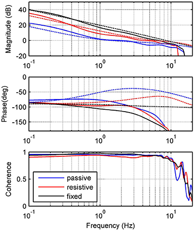
Figure 2. Experimental identification. Frequency response measurements of theoretical (dashed) and experimental (solid) transfer functions between input ${\omega }_m^d$ and output F_s. Graphs show responses for passive (blue), resistive (red) and fixed (black) modes.

Due to variations in the activation level of the muscles acting on the ankle joint, abrupt changes in ankle mechanical impedance are expected. In addition, operation modes defined are properly matched with the phases of human gait pattern. Thus, the fixed mode can be associated with the mid-stance phase; the resistive mode with the initial contact, terminal stance and double support of the stance phase; and the passive mode with the swing phase. Table 1 shows the platform specifications, as well as the human parameters used for each mode and their corresponding lower limits. Parameters for Mode 1 were chosen to satisfy Z_l → ∞, in order to obtain similar results to those presented in Robinson et al. (1999). For Modes 2 and 3, they were chosen from Lee et al. (2016) taking into account the actual human impedance during stance and swing phases of walking, respectively.

TABLE 1

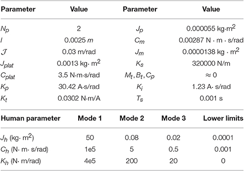
Table 1. Platform and human parameters.

3. Control Approaches

The block diagram of the control system for the SRPAR is presented in Figure 3. The platform uses an EPOS driver that performs two internal control loops for motor velocity and current. They are based on PI controllers with Kp and Ki gains shown in (see Table 1). Platform sensors provide data to a signal conditioning block where SRPAR-human system variables are computed. The sampling frequency used in this process is 1 kHz.

FIGURE 3

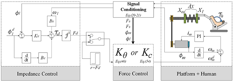
Figure 3. Overall control scheme for the SRPAR.

In order to ensure an appropriate interaction between human and platform, we implement a standard impedance control configuration for SEAs that uses the following internal force control law:

$\begin{array}{cc}{F}_d={{J}}^{-1}\left(K_v({\varphi }_l^d-{\varphi }_l)+B_v({\omega }_l^d-{\omega }_l)\right),& \left(22\right)\end{array}$

where F_d is the desired force computed from a sequence of desired trajectories for load angular position ${\varphi }_l^d$ and velocity ${\omega }_l^d$. It is determined by the virtual stiffness K_v and damping B_v.

We aim to improve the performance and to guarantee the stability of the system for different modes of human activities, where changes among them are modeled as random jumps. In this sense, we design a recursive robust regulator for discrete-time Markov jump linear systems (RR-DMJLS). Disturbances and uncertainties due to human-robot interactions, mainly because of human parameters (inertia, stiffness, and damping), are considered in this control approach. For comparison purposes, we also design an ${{H}}_{\infty }$ force controller that does not take into account these different modes of human activities. We synthesize a fixed-gain controller using a similar approach presented in Mehling and O'Malley (2014) and dos Santos et al. (2015). Both controllers are presented in the following.

3.1. Recursive RR-DMJLS Force Control Design

In this section, we design a robust force controller for the SRPAR (Figure 4A). We present first nominal and uncertain representations for different operation modes of the system. Then, we model the system as a discrete-time Markovian jump linear system (DMJLS). In order to guarantee stability and robust performance, we use the recursive RR-DMJLS algorithm developed in Cerri and Terra (2017).

FIGURE 4

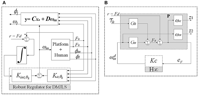
Figure 4. Force control approaches. (A) Recursive Robust Regulator for DMJLS: the block “Platform + Human” corresponds to the state variable model in Equation 20, K_int,θk and K_a,θk are the control gains. (B) ${{H}}_{\infty }$ control configuration of the system: G_n is the process plant, P is the augmented plant including the weight functions and K_c is the controller.

3.1.1. Nominal Model

Consider the model presented in Equation (20),

$\begin{array}{cc}{\dot{x}}_a=F_{a_{\theta }}{x}_a+B_{a_{\theta }}{w}_m+G_{a_{\theta }}{\tau }_h,& \left(23\right)\end{array}$

for each operation mode θ ∈ Θ: = {1, …, s}, where s is the number of nominal models, $F_{a_{\theta }}\in {ℝ}^{nxn}$, $B_{a_{\theta }}\in {ℝ}^{nxm}$, and $G_{a_{\theta }}\in {ℝ}^{nxm}$ are nominal parameter matrices, $x_a\in {ℝ}^n$ is the state vector, $w_m\in {ℝ}^m$ is the input control and ${\tau }_h\in {ℝ}^m$ is the input disturbance.

We discretized this model by using F_{aθ, k} = I + F_aθT_sΩ, B_{aθ, k} = ΩT_sB_aθ, and G_{aθ, k} = ΩT_sG_aθ, with $\Omega =\sum _{k_n=0}^9\frac{F_{a_{\theta }}^{k_n}{T}_s^{k_n}}{(k_n+1)!}$, where T_s = 1 ms is the sample time, for each k ∈ ℤ⁺. To eliminate the steady state error, we augment the model by including an integral action:

$\begin{array}{cc}\begin{array}{l}\underset{x_{k+1}}{\underbrace{\left[\begin{array}{c}{x}_{a_{k+1}}\\ x_{in{t}_{k+1}}\end{array}\right]}}=\underset{F_{\theta ,k}}{\underbrace{\left[\begin{array}{cc}{F}_{a_{\theta ,k}}& 0\\ C_a{T}_s& 1\end{array}\right]}}\underset{x_k}{\underbrace{\left[\begin{array}{c}{x}_{a_k}\\ x_{in{t}_k}\end{array}\right]}}+\underset{B_{\theta ,k}}{\underbrace{\left[\begin{array}{c}{B}_{a_{\theta ,k}}\\ 0\end{array}\right]}}\underset{u_k}{\underbrace{w_{m_k}}}\\ +\underset{B{r}_{\theta ,k}}{\underbrace{\left[\begin{array}{c}0\\ T_s\end{array}\right]}}{r}_k+\underset{G_{\theta ,k}}{\underbrace{\left[\begin{array}{c}{G}_{a_{\theta ,k}}\\ 0\end{array}\right]}}{\tau }_{h_k},\end{array}& \left(24\right)\end{array}$

where r_k is a force reference signal and C_a = [0 − 1 0 0]. F_{θ, k} and B_{θ, k} are nominal matrices for three nominal models according to Equation (20), which are based on parameters presented in Table 1:

$\begin{array}{cc}\begin{array}{l}\text{Mode 1: }{F}_{1,k}=\left[\begin{array}{ccccc}0.134& -3.81& 219& 0& 0\\ 4·{10}^{-4}& 0.998& 0.144& 0& 0\\ 0& 0& 1& 0& 0\\ 0& 0& -1·{10}^{-5}& 1& 0\\ 0& -0.001& 0& 0& 1\end{array}\right],\\ B_{1,k}=\left[\begin{array}{c}55.11\\ 0.036\\ 0.001\\ 3·{10}^{-6}\\ -1·{10}^{-5}\end{array}\right];\end{array}& \left(25\right)\end{array}$

$\begin{array}{cc}\begin{array}{l}\text{Mode 2: }{F}_{2,k}=\left[\begin{array}{ccccc}0.898& -4.26& 7.43& 0& 0\\ 9·{10}^{-4}& 0.998& 0.003& 0& 0\\ 0& 0& 1& 0& 0\\ 9·{10}^{-8}& 0& 0& 1& 0\\ 0& -0.001& 0& 0& 1\end{array}\right],\\ B_{2,k}=\left[\begin{array}{c}6.31\\ 0.003\\ 0.001\\ 6·{10}^{-6}\\ -1·{10}^{-6}\end{array}\right];\end{array}& \left(26\right)\end{array}$

$\begin{array}{cc}\begin{array}{l}\text{Mode 3: }{F}_{3,k}=\left[\begin{array}{ccccc}0.822& -13.1& 2.72& 0& 0\\ 9·{10}^{-3}& 0.993& 0.001& 0& 0\\ 0& 0& 1& 0& 0\\ 9·{10}^{-8}& 0& 0& 1& 0\\ 0& -0.001& 0& 0& 1\end{array}\right],\\ B_{3,k}=\left[\begin{array}{c}10.87\\ 0.005\\ 0.001\\ 6·{10}^{-6}\\ -2·{10}^{-6}\end{array}\right].\end{array}& \left(27\right)\end{array}$

3.1.2. Uncertain Model

Consider the system presented in Section 3.1.1 subject to parametric uncertainties given by:

$\begin{array}{cc}\begin{array}{l}\left[\begin{array}{c}{x}_{a_{k+1}}\\ x_{in{t}_{k+1}}\end{array}\right]=\underset{F_{\theta ,k}^{\delta }=F_{\theta ,k}+\delta F_{\theta ,k}}{\underbrace{\left[\begin{array}{cc}{F}_{a_{\theta ,k}}+\delta F_{{11}_{\theta ,k}}& \delta F_{{12}_{\theta ,k}}\\ C_a{T}_s+\delta F_{{21}_{\theta ,k}}& 1+\delta F_{{22}_{\theta ,k}}\end{array}\right]}}\left[\begin{array}{c}{x}_{a_k}\\ x_{in{t}_k}\end{array}\right]\\ +\underset{B_{\theta ,k}^{\delta }=B_{\theta ,k}+\delta B_{\theta ,k}}{\underbrace{\left[\begin{array}{c}{B}_{a_{\theta ,k}}+\delta B_{{11}_{\theta ,k}}\\ \delta B_{{21}_{\theta ,k}}\end{array}\right]}}{u}_k+\left[\begin{array}{c}0\\ T_s\end{array}\right]r_k\\ +\underset{G_{\theta ,k}^{\delta }=G_{\theta ,k}+\delta G_{\theta ,k}}{\underbrace{\left[\begin{array}{c}{G}_{a_{\theta ,k}}+\delta G_{{11}_{\theta ,k}}\\ \delta G_{{21}_{\theta ,k}}\end{array}\right]}}{\tau }_{h_k}.\end{array}& \left(28\right)\end{array}$

Uncertain matrices δF_{θ, k} and δB_{θ, k} are modeled by:

$\begin{array}{cc}\left[\delta F_{\theta ,k}\delta B_{\theta ,k}\right]=H_{\theta ,k}{\Delta }_{\theta ,k}\left[E_{F_{\theta ,k}}{E}_{B_{\theta ,k}}\right],& \left(29\right)\end{array}$

where $H_{\theta ,k}\in {ℝ}^{nxk}$ is a nonzero matrix, $E_{F_{\theta ,k}}\in {ℝ}^{lxn}$ and $E_{B_{\theta ,k}}\in {ℝ}^{lxm}$ are known matrices, Δ_{θ, k} is an arbitrary matrix that satisfies ||Δ_{θ, k}|| ≤ 1. In order to identify matrices H_{θ, k}, E_{Fθ, k} and E_{Bθ, k}, we analyze frequency responses of the nominal and uncertain models described in Equations (24) and (28), where τ_hk = 0, by:

$\begin{array}{cc}\begin{array}{l}{x}_n(z)={\left(zI-F_{\theta ,k}\right)}^{-1}(B_{\theta ,k}u(z)+B{r}_{\theta ,k}r(z)),\hfill \\ \to G_{n_{\theta }}(e^{j\omega T_s})={\left(e^{j\omega T_s}I-F_{\theta ,k}\right)}^{-1}[B_{\theta ,k}{B}_{r_{\theta ,k}}],\hfill \end{array}& (30)\end{array}$

$\begin{array}{cc}\begin{array}{l}{x}_{un}(z)={\left(zI-F_{\theta ,k}^{\delta }\right)}^{-1}(B_{\theta ,k}^{\delta }u(z)+B{r}_{\theta ,k}r(z)),\hfill \\ \to G_{u{n}_{\theta }}(e^{j\omega T_s})={\left(e^{j\omega T_s}I-F_{\theta ,k}^{\delta }\right)}^{-1}[B_{\theta ,k}^{\delta }{B}_{r_{\theta ,k}}],\hfill \end{array}& (31)\end{array}$

with $z=e^{j\omega T_s}\approx \frac{1+j\omega T_s/2}{1-j\omega T_s/2}$. For each operation mode, we compute a transfer function W_{a, θ} in order to satisfy:

$\begin{array}{cc}\Vert {\sigma }_{W_{a,\theta }(e^{j\omega T_s})}\Vert \ge \Vert {\sigma }_{G_{n_{\theta }}(e^{j\omega T_s})}-{\sigma }_{G_{u{n}_{\theta }}(e^{j\omega T_s})}\Vert ,\forall \omega & \left(32\right)\end{array}$

where σ_Gnθ and σ_Gunθ are singular values of the nominal and uncertain models, respectively, see Figure 5. Notice that upper bounds defined by singular values of W_{a, θ} are effective for frequencies until 1.7 Hz for resistive mode and 3.8 Hz for passive mode.

FIGURE 5

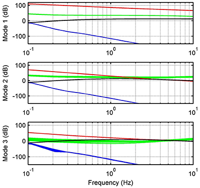
Figure 5. Relative errors and upper bounds. Relative errors between nominal and uncertain models with respect to inputs u_k (green) and r_k (blue). Graphs also show upper bounds for inputs u_k (red) and r_k (black).

Finally, matrices H_{θ, k}, E_{Fθ, k}, and E_{Bθ, k} are found using a genetic algorithm considering Equation (32):

$\begin{array}{cc}{H}_{1,k}=H_{2,k}=H_{3,k}={\left[\begin{array}{ccccc}-1187& -10.3& -0.5& {10}^5& 10\end{array}\right]}^T,& \left(33\right)\end{array}$

and

$\begin{array}{cc}\{\begin{array}{ll}{E}_{F_{1,k}}=\left[\begin{array}{ccccc}-0.86& -330.0& 0& 0& 1308\end{array}\right],\hfill & E_{B_{1,k}}=\left[\begin{array}{c}-118.00\end{array}\right],\text{ for Mode 1};\hfill \\ E_{F_{2,k}}=\left[\begin{array}{ccccc}-0.43& -661.0& 0& 72& 4448\end{array}\right],\hfill & E_{B_{2,k}}=\left[\begin{array}{c}-59.30\end{array}\right],\text{ for Mode 2};\hfill \\ E_{F_{3,k}}=\left[\begin{array}{ccccc}-0.31& -79.4& 0& 72& 3768\end{array}\right],\hfill & E_{B_{3,k}}=\left[\begin{array}{c}-47.46\end{array}\right],\text{ for Mode 3}.\hfill \end{array}& \left(34\right)\end{array}$

3.1.3. Probability Matrix

Time transitions among modes defined in Section 2.3 for the system presented in Equation (28) can be modeled by a Markov chain ${\left\{{\theta }_k\right\}}_{k=0}^{{N}-1}$, where θ_k is called the jump parameter and belongs to a finite set Θ: = {1, …, s}. Transitions among these different modes are determined by a probability matrix for state transitions $\mathbb{P}=\left[p_{ij,k}\right]\in {ℝ}^{s\times s}$ where each input must satisfies the following constraints:

$\begin{array}{cc}\begin{array}{l}Prob[{\theta }_{k+1}=j|{\theta }_k=i]=p_{ij,k},Prob[{\theta }_0=i]=p_{i,k},\\ {\displaystyle \sum _{j=1}^s{p}_{ij,k}}=1,0\le p_{ij,k}\le 1.\end{array}& \left(35\right)\end{array}$

ℙ is defined heuristically based on empirical observations of the respective operation modes:

$\begin{array}{cc}\mathbb{P}=\left[\begin{array}{ccc}0.95& 0.05& 0\\ 0& 0.9& 0.1\\ 0& 0.1& 0.9\end{array}\right].& \left(36\right)\end{array}$

Different intervals for load velocity and position can describe different behaviors of the human-robot system. Namely, if the user is passive (1), resistive (2) or if the platform is fixed (3), ω_l and ϕ_l provide the jump parameter where,

$\begin{array}{cc}{\theta }_k=\{\begin{array}{lll}1\hfill & \text{ if }\hfill & {\omega }_{l_k}^f\le 1\text{ and }|{\varphi }_{l_k}|<0.1,\hfill \\ 2\hfill & \text{ else if }\hfill & {\omega }_{l_k}^f\le 2\text{ and }|{\varphi }_{l_k}|\ge 0.1,\hfill \\ 3\hfill & \text{ else if }\hfill & {\omega }_{l_k}^f>2\text{ and }|{\varphi }_{l_k}|\approx 0,\hfill \end{array}& \left(37\right)\end{array}$

for each $k=0,\dots ,{N}-1$, where $w_{l_k}^f$ is the low-pass filtered signal from load velocity absolute value, with f_c = 0.1 Hz and T_s = 1 ms, given by:

$\begin{array}{cc}{w}_{l_k}^f=(1-\varrho )w_{l_{k-1}}^f+\varrho |w_{l_{k-1}}|,\text{ with }\varrho =2\pi f_c{T}_s.& \left(38\right)\end{array}$

Since w_lk is related to the frequency response of the system, the jump parameter θ_k is also related to the robustness of the regulator. In fact, robust stability and optimal performance is only guaranteed in the interval of frequencies in which relative errors are represented by upper bounds ||σ_{Wa, i(jω)}|| (Figure 5).

3.1.4. RR-DMJLS Algorithm

Equation (28) is rewritten as a discrete-time Markov jump linear system subject to parametric uncertainties, by:

$\begin{array}{cc}\begin{array}{l}{x}_{k+1}=\left(F_{{\theta }_k,k}+\delta F_{{\theta }_k,k}\right)x_k+\left(B_{{\theta }_k,k}+\delta B_{{\theta }_k,k}\right)u_k,\\ \text{with }{\theta }_k\in \{1,2,3\}\end{array}& \left(39\right)\end{array}$

for all $k=0,\dots ,{N}-1$, where F_{θk, k} and B_{θk, k} are nominal parameter matrices for each mode given by Equation (25), x_k is the state vector, u_k is an input control, and δF_{θk, k} and δB_{θk, k} are uncertain matrices modeled as:

$\begin{array}{cc}\left[\delta F_{{\theta }_k,k}\delta B_{{\theta }_k,k}\right]=H_{{\theta }_k,k}{\Delta }_{{\theta }_k,k}\left[E_{F_{{\theta }_k,k}}{E}_{B_{{\theta }_k,k}}\right],& \left(40\right)\end{array}$

according to parameters presented in Equations (33) and (34).

Consider the robust control problem to regulate the DMJLS subject to parametric uncertainties defined in Equation (39). The solution for this problem is achieved through the min-max optimization problem:

$\begin{array}{cc}\underset{x_{k+1},u_k}{\min }\underset{{}_{\delta F_{{\theta }_k,k},\delta B_{{\theta }_k,k}}}{\max }\{{\tilde{J}}_K^{\mu }(x_{k+1},u_k,\delta F_{{\theta }_k,k},\delta B_{{\theta }_k,k})\},& \left(41\right)\end{array}$

for each $k={N}-1,\dots ,0$ and θ_k ∈ Θ, where ${\tilde{J}}_K^{\mu }$ is the uncertain penalized-regularized quadratic functional:

$\begin{array}{cc}\begin{array}{l}{\tilde{J}}_K^{\mu }(x_{k+1},u_k,\delta F_{{\theta }_k,k},\delta B_{{\theta }_k,k})={\left[\begin{array}{c}{x}_{k+1}\\ u_k\end{array}\right]}^T\left[\begin{array}{cc}{\Psi }_{{\theta }_k,k+1}& 0\\ 0& R_{{\theta }_k,k}\end{array}\right]\\ \left[\begin{array}{c}{x}_{k+1}\\ u_k\end{array}\right]+(\left[\begin{array}{cc}0& 0\\ I& -B_{{\theta }_k,k}^{\delta }\end{array}\right]\left[\begin{array}{c}{x}_{k+1}\\ u_k\end{array}\right]\\ {-\left[\begin{array}{c}-I\\ F_{{\theta }_k,k}^{\delta }\end{array}\right]x_k)}^T\left[\begin{array}{cc}{Q}_{{\theta }_k,k}& 0\\ 0& \mu I\end{array}\right]\\ \left(\left[\begin{array}{cc}0& 0\\ I& -B_{{\theta }_k,k}^{\delta }\end{array}\right]\left[\begin{array}{c}{x}_{k+1}\\ u_k\end{array}\right]-\left[\begin{array}{c}-I\\ F_{{\theta }_k,k}^{\delta }\end{array}\right]x_k\right),\end{array}& \left(42\right)\end{array}$

where $F_{{\theta }_k,k}^{\delta }$ and $B_{{\theta }_k,k}^{\delta }$ are defined in Equation (28); ${\text{Ψ}}_{{\theta }_k,k+1}=\sum _{j=1}^s{P}_{j,k+1}{p}_{ij,k}$; P_{θk, k} is a positive definite matrix; Q_{θk, k} and R_{θk, k} are semi-definite weighting matrices. The solution to the optimization problem expressed in Equations (41) and (42) that guarantees the optimal state-control sequence ${\left\{(x_{\mu ,k+1}^{*},u_{\mu ,k}^{*})\right\}}_{k=0}^{N-1}$ for a fixed instant k and state θ_k, is given by the following Robust Regulator for Discrete Markov Jump Linear Systems (RR-DMJLS):

Robust Regulator for DMJLS (Cerri and Terra, 2017).

Initial Conditions: Set x₀, θ₀, ℙ, $P_i({N})\succ 0$, ∀i ∈ Θ: = {1, …, s}.

Step 1: (Backward). Calculate for all $k={N}-1,\dots ,0$:

$\begin{array}{cc}\begin{array}{l}{\Psi }_{i,k+1}={\displaystyle \sum _{j=1}^s}{P}_{j,k+1}{p}_{ij,k}\\ \left[\begin{array}{c}{L}_{\mu ,i,k}\\ K_{\mu ,i,k}\\ P_{\mu ,i,k}\end{array}\right]={\left[\begin{array}{ccc}0& 0& 0\\ 0& 0& 0\\ 0& 0& -I\\ 0& 0& {\widehat{F}}_{i,k}\\ I& 0& 0\\ 0& I& 0\end{array}\right]}^T{\left[\begin{array}{cccccc}{\Psi }_{i,k+1}^{-1}& 0& 0& 0& I& 0\\ 0& R_{i,k}^{-1}& 0& 0& 0& I\\ 0& 0& Q_{i,k}^{-1}& 0& 0& 0\\ 0& 0& 0& {{W}}_{i,k}& \widehat{I}& -{\widehat{B}}_{i,k}\\ I& 0& 0& {\widehat{I}}^T& 0& 0\\ 0& I& 0& -{\widehat{B}}_{i,k}^T& 0& 0\end{array}\right]}^{-1}\\ \left[\begin{array}{c}0\\ 0\\ -I\\ {\widehat{F}}_{i,k}\\ 0\\ 0\end{array}\right],\end{array}& \left(43\right)\end{array}$

Step 2: (Forward). Obtain for each $k=0,\dots {N}-1$:

$\left[\begin{array}{c}{x}_{k+1}^{*}\\ u_k^{*}\end{array}\right]=\left[\begin{array}{c}{L}_{\mu ,i,k}\\ K_{\mu ,i,k}\end{array}\right]x_k^{*}$.

Equation (43) uses the following auxiliary matrices:

$\begin{array}{cc}\begin{array}{l}\begin{array}{c}{{W}}_{i,k}\end{array}=\left[\begin{array}{cc}{\mu }^{-1}I-{\widehat{\lambda }}_{i,k}^{-1}{H}_{{\theta }_k,k}{H}_{{\theta }_k,k}^T& 0\\ 0& {\widehat{\lambda }}_{i,k}^{-1}I\end{array}\right],\\ \widehat{I}=\left[\begin{array}{c}I\\ 0\end{array}\right],{\widehat{B}}_{i,k}=\left[\begin{array}{c}{B}_{{\theta }_k,k}\\ E_{B_{{\theta }_k,k}}\end{array}\right],{\widehat{F}}_{i,k}=\left[\begin{array}{c}{F}_{{\theta }_k,k}\\ E_{F_{{\theta }_k,k}}\end{array}\right],\\ {\lambda }_{i,k}>\parallel \mu H_{{\theta }_k,k}^T{H}_{{\theta }_k,k}\parallel .\end{array}& \left(44\right)\end{array}$

In this formulation, μ > 0 is a penalty parameter responsible to guarantee the robustness of the RR-DMJLS. In fact, when μ → +∞ then ${{W}}_{i,k}\to 0$. In consequence, the DMJLS closed-loop response is given by:

$\begin{array}{cc}\{\begin{array}{c}{L}_{\infty ,{\theta }_k,k}=F_{{\theta }_k,k}+B_{{\theta }_k,k}{K}_{\infty ,{\theta }_k,k}\\ E_{F_{{\theta }_k,k}}+E_{B_{{\theta }_k,k}}{K}_{\infty ,{\theta }_k,k}=0,\end{array}& \left(45\right)\end{array}$

which provides the robust optimal response $(x_{k+1}^{*},u_k^{*})$. Details of the necessary and sufficient conditions for existence of the mean square stabilizing solution and robustness of this regulator can be found in Cerri and Terra (2017).

Let μ = 9.998 × 10⁶ and ${\lambda }_{i,k}=1\times {10}^{17}$ in order to satisfy Equations (44) and (45); weighting matrices R_{1, k} = R_2,k = R_3,k = 1, Q_1,k = Q_2,k = Q_3,k = I₅ and $P_1({N})=P_2({N})=P_3({N})=1\times 10^{10}\times I_5$; and the probability matrix ℙ defined in Equation (36). By using the robust regulator presented in Equation (43), we obtain the following control law:

$\begin{array}{cc}{u}_k=K_{\infty ,{\theta }_k,k}{x}_k=K_{a,{\theta }_k}{x}_{a_k}+K_{int,{\theta }_k}{x}_{in{t}_k},& \left(46\right)\end{array}$

where K_a,θk is the gain to the states x_ak and K_int,θk is the gain to the state x_intk. Table 2 shows the control gains obtained for three Markovian modes. We do not consider uncertainties in the third term of E_Fi,k, as a consequence, the algorithm decouples the state variable ϕ_m guaranteeing the controllability of the system (see K₃).

TABLE 2

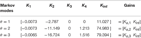
Table 2. Control gains.

Considering the control law presented in Equation (46), the closed-loop response for Equation (28) without considering the disturbance τ_hk, is given by:

$\begin{array}{cc}\begin{array}{l}\left[\begin{array}{c}{x}_{a_{k+1}}\\ x_{in{t}_{k+1}}\end{array}\right]=\underset{F_{\theta ,k}+B_{\theta ,k}{K}_{{\theta }_k}}{\underbrace{\left[\begin{array}{cc}{F}_{a_{\theta ,k}}+B_{a_{\theta ,k}}{K}_{a,{\theta }_k}& B_{a_{\theta ,k}}{K}_{int,{\theta }_k}\\ C_a{T}_s& 1\end{array}\right]}}\left[\begin{array}{c}{x}_{a_k}\\ x_{in{t}_k}\end{array}\right]+B_{r_{\theta ,k}}{r}_k+\\ \underset{\delta F_{\theta ,k}+\delta B_{\theta ,k}{K}_{{\theta }_k}=H_k{\Delta }_k(E_{F_k}+E_{B_k}{K}_{\infty ,{\theta }_k,k})=0}{\underbrace{\left[\begin{array}{cc}\delta F_{{11}_{\theta ,k}}+\delta B_{{11}_{\theta ,k}}{K}_{a,{\theta }_k}& \delta F_{{12}_{\theta ,k}}+\delta B_{{11}_{\theta ,k}}{K}_{int,{\theta }_k}\\ \delta F_{{21}_{\theta ,k}}+\delta B_{{21}_{\theta ,k}}{K}_{a,{\theta }_k}& \delta F_{{22}_{\theta ,k}}+\delta B_{{21}_{\theta ,k}}{K}_{int,{\theta }_k}\end{array}\right]}}\left[\begin{array}{c}{x}_{a_k}\\ x_{in{t}_k}\end{array}\right],\end{array}& \left(47\right)\end{array}$

where δF_k + δB_kK_∞,θk,k = 0 guarantees the robustness of the system according to Equation (45).

3.2. ${{H}}_{\infty }$ Force Control Design

Consider the nominal model:

$\begin{array}{cc}{G}_n(s)=\frac{\rho N_p{K}_s{K}_t{K}_{PI}}{K_{PI}{M}_{meq}{s}^2+K_{PI}{B}_{meq}s+K_s}.& \left(48\right)\end{array}$

We use a mixed-sensitivity shaping approach $S={(1+G_n{K}_c)}^{-1}$ to ensure tracking performance and disturbance rejection, and K_cS to limit the control signal (Skogestad and Postlethwaite, 2007). The ${{H}}_{\infty }$ problem is defined as:

$\begin{array}{cc}\begin{array}{l}\underset{K_c}{\min }\Vert \mathbb{N}(K_c){\Vert }_{\infty },\mathbb{N}={\left[\begin{array}{cc}{w}_{e}S& w_u{K}_{c}S\end{array}\right]}^T={\left[\begin{array}{cc}{z}_1& z_2\end{array}\right]}^T,\\ \Vert \mathbb{N}{\Vert }_{\infty }=\underset{\omega }{\max }\overline{\sigma }(\mathbb{N}(j\omega ))\le \gamma ,\end{array}& \left(49\right)\end{array}$

where w_e(s) and w_u(s) are respectively performance and control weights, K_c is a stabilizing controller that bounds ℕ by an attenuation level γ, and $\bar{\sigma }(\mathbb{N})$ is given by the usual Euclidean vector norm:

$\begin{array}{cc}\overline{\sigma }(\mathbb{N})=\sqrt{|w_{e}S{|}^2+|w_u{K}_{c}S{|}^2}.& \left(50\right)\end{array}$

We define the performance weighting w_e(s) by:

$\begin{array}{cc}{w}_e=\frac{\text{s}/{10}^{(Ms/20)}+{\omega }_b}{\text{s}+{\omega }_b{ϵ}_s},& \left(51\right)\end{array}$

where ${ϵ}_s=10^{-5}$ is the maximum steady-state error, M_s = 2 dB is the maximum peak of S, and ω_b = 10π is related to the close-loop bandwidth. We determine the control input weighting w_u(s) with

$\begin{array}{cc}{w}_u=1/M_u,& \left(52\right)\end{array}$

where M_u = 523.6 rad/s (5,000 rpm) is the maximum value for u. The control system is considered according to Figure 4B. Based on Equations (51) and (52), the ${{H}}_{\infty }$ force controller K_c(s) is obtained:

$\begin{array}{cc}{K}_c(s)=\frac{2.78\text{e}9s^3+2.18\text{e}12s^2+6.95\text{e}13s+6.95\text{e}10}{s^4+5.52\text{e}6s^3+3.34\text{e}11s^2+1.35\text{e}13s+4.3\text{e}6}.& \left(53\right)\end{array}$

Finally, the controller is discretized by using a zero-order hold, with T_s = 1 ms,

$\begin{array}{cc}{K}_c(z)=\frac{6.16z^2-12.11z+5.95}{z^3-1.96z^2+0.96z}.& \left(54\right)\end{array}$

4. Experimental Results

In order to evaluate the stability and performance of the proposed control approaches, time and frequency response tests are performed with a healthy user for three different operation modes presented in Section 2.3. We show a comparative study of force controllers and impedance controllers, according to Figure 4. This study was approved and carried out in accordance with the recommendations of the Ethics Committee of the Federal University of São Carlos (Number 26054813.1.0000.5504).

4.1. Force Controllers

In this section, robust force controllers presented in Section 3, RR-DMJLS and ${{H}}_{\infty }$, are compared. Two performance criteria are used for this purpose. We consider the rise time t_r and a normalized mean error between spring and desired forces defined as

$\begin{array}{cc}{e}_{qc}=\frac{1}{N}{\displaystyle \sum _{k=1}^N\left|\frac{F_d-F_s}{max\left\{F_d\right\}}\right|}·100\%,& \left(55\right)\end{array}$

where N = 8/T_s is the number of samples.

Figure 6 shows time responses of the system using the RR-DMJLS force controller. In these experiments, three different levels (100, 0, and − 100 N) of desired forces, F_d, are set during a total time of T = 8 s. In tests performed for fixed and resistive modes, shown in Figures 6A,B, the Markovian modes remained constant. Notice in the test shown in Figure 6C, the Markov chain changes between Modes 2 and 3. The RR-DMJLS responses are similar for three modes available, maintaining an appropriate tracking despite natural differences between human and robot dynamics. Notice that t_r are similar to the respective desired force levels and the mean errors e_qc are 14.24, 11.97, and 11.9%, for tests shown in Figures 6A–C, respectively.

FIGURE 6

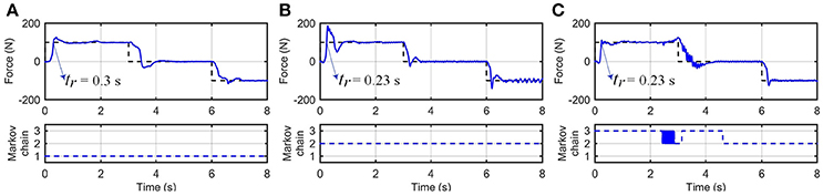
Figure 6. Recursive RR-DMJLS force controller. (A) Fixed mode. (B) Resistive mode. (C) Resistive and passive modes. For each operation mode, graphs show desired (black) and actual (blue) spring forces (top), and Markov chains (bottom).

Figure 7 shows the force control response of the RR-DMJLS while tracking a sinusoidal force reference. In this experiment, the user is asked to be resistive to the movement of the platform during the first fifteen seconds, and then to remain passive during the next fifteen seconds. We observe that force control maintains a similar response despite the abrupt change in the human dynamics (resistive → passive). Notice that jumps between Markovian states reflect time transitions between different operation modes of the system. However, for a condition where the operation modes change more frequently, these transitions would be detected with a certain delay. We hypothesize that this delay is related to the jump parameter identification method considered (Equation 37). It could be improved by estimating alternative variables. For example, the stiffness and damping parameters of the human being.

FIGURE 7

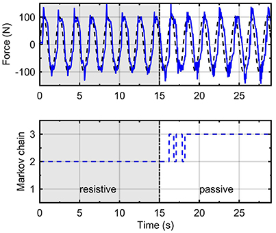
Figure 7. Recursive RR-DMJLS force controller. Force response (solid), sinusoidal force reference (dashed) with a change of operation mode (top). Markov chain (bottom).

Figure 8 presents time responses of the system using the ${{H}}_{\infty }$ force control approach. In this case, also are applied three different levels of desired forces F_d in T = 8 s, for each operation mode: fixed, resistive, and passive. The rise time t_r is lower for fixed and resistive modes in comparison with the passive mode. The mean errors obtained for fixed, resistive and passive modes were 5.89, 8.23, and 23.29%, respectively. Comparing mean errors between both controllers, we obtain better performance for the ${{H}}_{\infty }$ force controller for the fixed mode. For the passive mode, the RR-DMJLS provides better performance. However, when we design the ${{H}}_{\infty }$ control based on the passive mode, it does not stabilize the system when it is operating in the fixed mode. An advantage of the RR-DMJLS is the uniformity of performance obtained for the whole system.

FIGURE 8

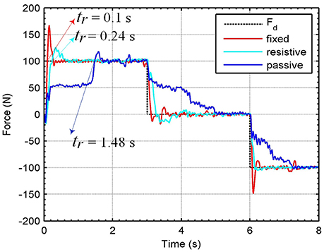
Figure 8. Time response of the system with ${{H}}_{\infty }$ force controller.

Figure 9 shows frequency responses of the closed-loop system using the ${{H}}_{\infty }$ and recursive RR-DMJLS force controllers. For passive and resistive modes, we apply a desired force signal given by a chirp signal with amplitude of 100 N, sweeping frequencies between 0 and 8 Hz. Some indexes for both controllers are compared. For the ${{H}}_{\infty }$ force controller, shown in Figure 9A, we have: maximum magnitude during passive mode, |G_fp|_max = −1.6 dB, and resistive mode, |G_fr|_max = 0.86 dB; bandwidth for passive mode, B_wfp−3dB = 0.2 Hz, and bandwidth for resistive mode, B_wfr−3dB = 1.39 Hz; phase at cut-off frequency for passive mode, ${\alpha }_{fp}=-43^{°}$, and for resistive mode, ${\alpha }_{fr}=-79^{°}$. For the frequency response of the RR-DMJLS shown in Figure 9B, we obtain: |_Gfp|max = 0.9 dB; |_Gfr|max = 0.32 dB; B_wfp−3dB = 1.2 Hz; B_wfr−3dB = 1.5 Hz; ${\alpha }_{fp}=-110^{°}$; and ${\alpha }_{fr}=-75^{°}$. Notice that the bandwidth of the closed-loop system is greater for the RR-DMJLS controller.

FIGURE 9

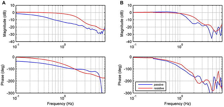
Figure 9. Frequency closed-loop response of the system with force control. (A) ${{H}}_{\infty }$ force control. (B) Recursive RR-DMJLS force control. Graphs show responses for passive (blue) and resistive (red) modes.

4.2. Impedance Control

To obtain the RR-DMJLS force control response during impedance controlled movements, we perform two experiments in which the system must track a kinematic reference. In both cases, the user was asked to be resistive during first ten seconds and then to be passive during the next ten seconds. Figure 10A shows the force and impedance control for a pure stiffness control configuration and Figure 10B a stiffness-damping control configuration. Notice that the torque tracking performance is similar for two modes in spite of the transition between them. Regarding the passive case, the position tracking is better for the pure-stiffness configuration. However, since this configuration has no damping parameter, the velocity tracking is worse. We can include a damping coefficient. However, it can decrease the performance of the position tracking. Thus, there exists a compromise between these control objectives that must be considered by the assistance strategy. Regarding the Markovian states, notice that increasing B_v it reduces the velocity of the system and enforces the system to remain in the same Markovian state, Figure 10B.

FIGURE 10

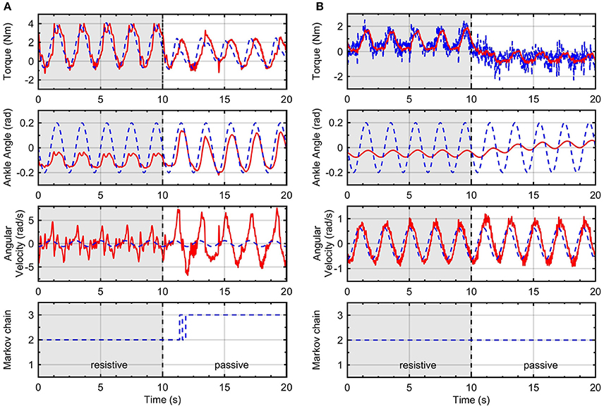
Figure 10. Impedance control with inner RR-DMJLS force control. Torque and impedance control responses for: (A) K_v = 15 N·m/rad and B_v = 0 N·m·s/rad, and (B) K_v = 15 N·m/rad and B_v = 5 N·m·s/rad. Graphs show desired (blue) and measured (red) values for the platform torque (top), angular position of the ankle joint (middle-top), angular velocity of the ankle joint (middle-bottom); and Markov chain (bottom).

Figure 11 shows time responses using the impedance control with the inner ${{H}}_{\infty }$ force control loop, for K = 15 N·m/rad, following a sinusoidal trajectory for ankle angular position. In this case, the user is asked to remain passive during the first ten seconds, and then to be resistive during the next ten seconds. Results show that the torque tracking performance is worse when the human being is in passive mode.

FIGURE 11

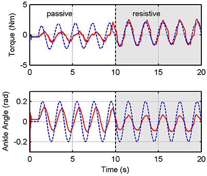
Figure 11. Impedance control with inner ${{H}}_{\infty }$ force control. Graphs show desired (blue) and measured (red) values for the platform torque, τ_plat (top), and angular position of the ankle joint (bottom).

In order to quantify the performance achieved by the proposed controllers, we compute the real stiffness and damping parameters of the system. For this purpose, we calculate the torque τ_Kv generated by the virtual stiffness K_v and the torque τ_Bv generated by the virtual damping B_v with

$\begin{array}{cc}{\tau }_{K_v}={\tau }_{plat}-B_v{\omega }_e\text{ and }{\tau }_{B_v}={\tau }_{plat}-K_v{\varphi }_e,& \left(56\right)\end{array}$

where ${\varphi }_e={\varphi }_l^d-{\varphi }_l$ is the angular position error and ${\omega }_e={\omega }_l^d-{\omega }_l$ is the angular velocity error. We compute the root mean square (RMS) errors of the measured variables in the experiments shown in Figures 10, 11. The RMS of the angular error ϕ_e is given by:

$\begin{array}{cc}\text{RMS}\{{\varphi }_e\}=\sqrt{\frac{1}{N}{\displaystyle \sum _{k=1}^N{\varphi }_{e_k}^2}},& \left(57\right)\end{array}$

where N = 10/T_s is the number of samples in each test (passive or resistive). In a similar way, we calculate RMS values for angular velocity error ω_e, torque generated by virtual stiffness τ_Kv, and damping τ_Bv. Notice that, when B_v = 0 then τ_Bv = 0 and τ_Kv = τ_plat. Actual stiffness K_r and damping B_r are given by:

$\begin{array}{cc}{K}_r=\frac{\text{RMS}\left\{{\tau }_{K_v}\right\}}{\text{RMS}\left\{{\varphi }_e\right\}}\text{ and }{B}_r=\frac{\text{RMS}\left\{{\tau }_{B_v}\right\}}{\text{RMS}\left\{{\omega }_e\right\}},& \left(58\right)\end{array}$

see Table 3. The error between the virtual stiffness and the actual stiffness are calculated, e_Kv = |(K_v − K_r)/K_v|100% and the error between the virtual damping and the actual damping, e_Bv = |(B_v − B_r)/B_v|100%. We compare results of the impedance control with K_v = 15 Nm/rad and B_v = 0 Nms/rad. Impedance control with RR-DMJLS presents higher stiffness accuracy in both passive and resistive modes, 15.28 Nm/rad and 16.13 Nm/rad, respectively. With ${{H}}_{\infty }$ controller, it provides 16.44 Nm/rad in passive mode and 7 Nm/rad in resistive mode. Stiffness errors e_Kv of the RR-DMJLS force control are smaller than the ${{H}}_{\infty }$ force control. This difference can be seen in the passive mode (θ = 3), where the e_Kv error of the ${{H}}_{\infty }$ is approximately seven times greater than the RR-DMJLS. In the test with K_v = 15N·m/ rad and B_v = 5N·m·s/ rad, the performance is preserved.

TABLE 3

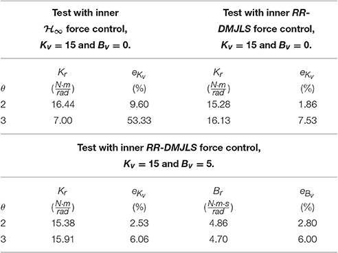
Table 3. Experimental measurements of the system stiffness and damping.

Figure 12 shows the frequency response for the impedance which is measured between output torque and angular position error. For passive and resistive modes, we apply a desired angular position trajectory given by a chirp signal with amplitude 0.2 rad, sweeping frequencies between 0 and 8 Hz. In these experiments, impedance controller is defined as pure stiffness configuration; therefore, magnitude of the impedance should be almost constant. Notice that it is guaranteed only until 1 Hz. Figure 12A shows the behavior of the RR-DMJLS-based impedance control. Figure 12B shows the frequency response for the ${{H}}_{\infty }$-based impedance control. Notice for this controller that the performance decreases when the system operates in the passive mode. We can see that the RR-DMJLS is a more resilient impedance control if compared with ${{H}}_{\infty }$-based control for different operating modes and desired impedances.

FIGURE 12

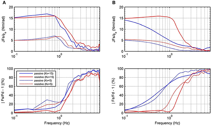
Figure 12. Frequency response for the measured impedance, ${J}{F}_s/{\varphi }_e$, and force error, |F_s/F_d − 1| · 100%, for K_v = 15, K_v = 5 and B_v = 0. (A) Inner recursive RR-DMJLS force control. (B) Inner ${{H}}_{\infty }$ force control.

5. Discussion and Conclusions

The model-based robust force control approach was evaluated in a robotic platform for ankle rehabilitation, improving its impedance control performance. First, the robot-human dynamics was modeled considering the ankle impedance a second-order system with inertia, stiffness, and damping parameters. Since we do not have exact knowledge of the human parameters, our system is subject to parametric uncertainties and we have defined three operation modes related to the human-robot activity whose time transitions were modeled via a Markov chain. For comparison purposes, an ${{H}}_{\infty }$ force controller was also evaluated. Although it can guarantee coupled stability, the force control performance decreases when the system is in the passive operation mode. We have also designed and implemented an RR-DMJLS for dealing with abrupt changes and system uncertainties by guaranteeing robust mean square stability of the system. Experimental results show RR-DMJLS outperformed the ${{H}}_{\infty }$ force controller.

5.1. Related Work

The impedance control configuration used is based on Hogan (1985) and it is aimed at the regulation of the dynamical behavior in the interaction port by variables that do not depend on the environment. The actuator together with the controller are modeled as an impedance, Z_r, with velocity inputs (angular) and force outputs (torque). The environment is considered an admittance, Y_e, in the interaction port. Colgate and Hogan (1988, 1989) presented sufficient conditions for the determination of stability of two coupled systems and explained how two physically coupled systems with Z_r and Y_e with passive port functions can guarantee stability. These concepts have been useful for the implementation of interaction controls for almost three decades. The stability of two coupled systems is given by Z_r and Y_e eigenvalues and the performance is evaluated by through the impedance Z_r.

Buerger and Hogan (2007) described a methodology in which an interaction control is designed for a robot module used for rehabilitation purposes. They considered an environment with restricted uncertain characteristics, therefore the admittance is rewritten as Y_e(s) = Y_n(s) + W(s)Δ(s). The authors also used a second-order dynamics to model the stiffness, damping, and inertia of the human parameters. Complementary stability for interacting systems was defined, where stability is determined by an environment subject to uncertainties. Therefore, a coupled stability problem is considered a robust stability problem.

Regarding the human modeling, the dynamic properties of the lower limbs and muscular activities vary considerably among subjects. This is relevant since SRPAR has been designed for users that suffer diseases that affect the human motor control system, e.g., stroke and other conditions that cause hemiplegia. Typically, such diseases change stiffness and damping in the ankle and knee joints, hence producing spasticity or hypertonia (Lin et al., 2006; Chow et al., 2012). Therefore, the development of a control strategy that guarantees a safe interaction between patient and platform, mainly in virtue of uncertainties related to the human being, is fundamental.

Li et al. (2017) and Pan et al. (2017) proposed adaptive control schemes for SEA-driven robots. They considered two operation modes in the adaptation process, namely robot-in-charge and human-in-charge, which are close related to the passive and resistive operation modes, respectively, proposed in this paper. However, the control adaptation is based on changes in the desired position input of the SEA controller and estimation of coordinate accelerations through nonlinear filtering.

In human-robot interaction control systems, the efficiency of the force actuator operation deserves special attention. Although SEAs are characterized by a low output impedance, an important requirement for improving such efficiency is the achievement of a precise and proportional output torque with respect to the desired input. Pratt (2002), Au et al. (2006), Kong et al. (2009), Mehling and O'Malley (2014), and dos Santos et al. (2015) developed force controllers for ankle actuators using SEA. In this paper, we proposed a force control methodology that can deal with system uncertainties and guarantee robust mean square stability. Similar performance was obtained in different tests performed. Accuracies of 98.14% for resistive mode and 92.47% for passive mode were obtained in the pure stiffness configuration. In the stiffness-damping configuration, with K_v = 15 and B_v = 5, the accuracy obtained in the resistive case was of 97.47% for stiffness and 97.2% for damping, and in the passive case was of 93.94% for stiffness and 94% for damping.

On the contrary, using a fixed-gain control approach based on ${{H}}_{\infty }$ synthesis, the performance was not similar among operation modes. We showed that this strategy can guarantee coupled stability; nevertheless, force control performance decreases when the system is in the passive operation mode. This is reflected in the impedance control accuracy for the pure stiffness configuration, falling from 90.4% in the resistive mode to 46.67% in the passive mode.

5.2. Shortcomings and Possible Improvements

In order to control the SRPAR, we proposed a methodology to force control based on RR-DMJLS. It considers a discrete-time Markovian model with three states associated with the operating modes of the system. The model was augmented for eliminating the steady state error through the inclusion of an integral action. We also found appropriate uncertain matrices considering frequency responses for relative errors between perturbed and nominal models.

Regarding the observation of the operation modes, in Figure 10A there exists a delay in the jump identification from resistive to passive mode, and in Figure 10B the proposed jump identification method was not even able to identify the jump between modes. This behavior is directly related to virtual damping B_v selected since load angular velocity $w_{l_k}^f$ is lower than 2 rad/s. A possible solution to the problem is the estimation of the virtual stiffness and damping of the human being for the definition of the bounds of the identification method.

Based on our observations of the system behavior, we have defined a probability matrix ℙ that models those transitions among different modes. We hypothesize the probabilities may vary in function of the user's physiological conditions, therefore, our probability matrix can be considered partially or completely uncertain. In a future study, we aim at using our methodology subject to uncertain transition probabilities with the unknown Markov chain proposed in Bortolin and Terra (2016).

Other approaches may improve our methodology. For example, a disturbance observer, as proposed in Kong et al. (2009), could compensate the effect of human torque τ_h in Equations (14) and (20). Optimal robust filter for DMJLS (Ishihara et al., 2015) and extended robust Kalman filter proposed in Inoue et al. (2016) could better estimate the states of the SRPAR.

Author Contributions

AJ, JJ, FE, and JP conceived research, performed the experiments and the data analysis, drafted the manuscript, and coded the controllers. MT and AS participated in the design of the controllers and in the draft of the manuscript. All authors read and approved the final manuscript.

Funding

This research is supported by Office of Research Administration of University of São Paulo, Coordination for Improvement of Higher Education Personnel (CAPES), Colciencias (Colombia), National Council for Scientific and Technological Development (CNPq) under grants 132221/2013-6 and 142080/2016-0, and São Paulo Research Foundation (FAPESP) under grants 2011/04074-3 and 2013/14756-0.

Conflict of Interest Statement

The authors declare that the research was conducted in the absence of any commercial or financial relationships that could be construed as a potential conflict of interest.

References

Au, S. K., Dilworth, P., and Herr, H. (2006). “An ankle-foot emulation system for the study of human walking biomechanics,” in Proceedings 2006 IEEE International Conference on Robotics and Automation, 2006. ICRA 2006 (Orlando, FL), 2939–2945.

Google Scholar

Bortolin, D. C., and Terra, M. H. (2016). “Recursive robust regulator for markovian jump linear systems subject to uncertain transition probabilities with unknown markov chain,” in 2016 IEEE Conference on Control Applications (CCA), 774–779. doi: 10.1109/CCA.2016.7587912

CrossRef Full Text | Google Scholar

Buerger, S. P., and Hogan, N. (2007). Complementary stability and loop shaping for improved human ndash;robot interaction. IEEE Trans. Robot. 23, 232–244. doi: 10.1109/TRO.2007.892229

CrossRef Full Text | Google Scholar

Calanca, A., Capisani, L., and Fiorini, P. (2014). Robust force control of series elastic actuators. Actuators 3, 182–204. doi: 10.3390/act3030182

CrossRef Full Text | Google Scholar

Calanca, A., Muradore, R., and Fiorini, P. (2016). A review of algorithms for compliant control of stiff and fixed-compliance robots. IEEE/ASME Trans. Mechatr. 21, 613–624. doi: 10.1109/TMECH.2015.2465849

CrossRef Full Text | Google Scholar

Cattaneo, D., Nuzzo, C. D., Fascia, T., Macalli, M., Pisoni, I., and Cardini, R. (2002). Risks of falls in subjects with multiple sclerosis. Arch. Phys. Med. Rehabil. 83, 864–867. doi: 10.1053/apmr.2002.32825

PubMed Abstract | CrossRef Full Text | Google Scholar

Cerri, J. P., and Terra, M. H. (2017). Recursive robust regulator for discrete-time Markovian jump linear systems. IEEE Trans. Autom. Control. doi: 10.1109/TAC.2017.2707335

CrossRef Full Text | Google Scholar

Chang, W. H., and Kim, Y.-H. (2013). Robot-assisted therapy in stroke rehabilitation. J. Stroke 15, 174–181. doi: 10.5853/jos.2013.15.3.174

PubMed Abstract | CrossRef Full Text | Google Scholar

Chow, J. W., Yablon, S. A., and Stokic, D. S. (2012). Coactivation of ankle muscles during stance phase of gait in patients with lower limb hypertonia after acquired brain injury. Clin. Neurophysiol. 123, 1599–1605. doi: 10.1016/j.clinph.2012.01.006

PubMed Abstract | CrossRef Full Text | Google Scholar

Colgate, E., and Hogan, N. (1989). The Interaction of Robots with Passive Environments: Application to Force Feedback Control. Berlin; Heidelberg: Springer.

Google Scholar

Colgate, J. E., and Hogan, N. (1988). Robust control of dynamically interacting systems. Int. J. Control 48, 65–88. doi: 10.1080/00207178808906161

CrossRef Full Text | Google Scholar

dos Santos, W. M., Caurin, G. A., and Siqueira, A. A. (2015). Design and control of an active knee orthosis driven by a rotary series elastic actuator. Control Eng. Pract. 58, 307–318. doi: 10.1016/j.conengprac.2015.09.008

CrossRef Full Text | Google Scholar

Gonçalves, A., Siqueira, A. A., dos Santos, W. M., Consoni, L. J., do Amaral, L. M., and de OB Franzolin, S. (2013). “Development and evaluation of a robotic platform for rehabilitation of ankle movements,” in 22st International Congress Of Mechanical Engineering (Ribeirão Preto), 8291–8298.

Gonçalves, A. C. B. F., dos Santos, W. M., Consoni, L. J., and Siqueira, A. A. G. (2014). “Serious games for assessment and rehabilitation of ankle movements,” in Serious Games and Applications for Health (SeGAH), 2014 IEEE 3rd International Conference on (Rio de Janeiro), 1–6.

Hatano, S. (1976). Experience from a multicentre stroke register: a preliminary report. Bull. World Health Organ. 54, 541–553.

PubMed Abstract | Google Scholar

Hogan, N. (1985). Impedance control: an approach to manipulation. J. Dyn. Syst. Measure. Control 107(Pt. 1–3), 1–24. doi: 10.1115/1.3140702

CrossRef Full Text

Inoue, R. S., Terra, M. H., and Cerri, J. P. (2016). Extended robust kalman filter for attitude estimation. IET Control Theory Appl. 10, 162–172. doi: 10.1049/iet-cta.2015.0235

CrossRef Full Text | Google Scholar

Ishihara, J. Y., Terra, M. H., and Cerri, J. P. (2015). Optimal robust filtering for systems subject to uncertainties. Automatica 52, 111–117. doi: 10.1016/j.automatica.2014.10.120

CrossRef Full Text | Google Scholar

Jutinico, A. L., Jaimes, J. C., Escalante, F. M., Perez-Ibarra, J. C., Terra, M. H., and Siqueira, A. A. G. (2017). “Recursive robust regulator for discrete-time markovian jump linear systems: control of series elastic actuators,” in 20th IFAC World Congress (Toulouse).

Kong, K., Bae, J., and Tomizuka, M. (2009). Control of rotary series elastic actuator for ideal force-mode actuation in human 2013;robot interaction applications. IEEE/ASME Trans. Mechatr. 14, 105–118. doi: 10.1109/TMECH.2008.2004561

CrossRef Full Text | Google Scholar

Krebs, H. I., Dipietro, L., Levy-Tzedek, S., Fasoli, S. E., Rykman-Berland, A., Zipse, J., et al. (2008). A paradigm shift for rehabilitation robotics. IEEE Eng. Med. Biol. Mag. 27, 61–70. doi: 10.1109/MEMB.2008.919498

PubMed Abstract | CrossRef Full Text | Google Scholar

Lee, H., Rouse, E. J., and Krebs, H. I. (2016). Summary of human ankle mechanical impedance during walking. IEEE J. Transl. Eng. Health Med. 4, 1–7. doi: 10.1109/JTEHM.2016.2601613

PubMed Abstract | CrossRef Full Text | Google Scholar

Li, X., Pan, Y., Chen, G., and Yu, H. (2017). Adaptive human-robot interaction control for robots driven by series elastic actuators. IEEE Trans. Robot. 33, 169–182. doi: 10.1109/TRO.2016.2626479

CrossRef Full Text | Google Scholar

Lin, P.-Y., Yang, Y.-R., Cheng, S.-J., and Wang, R.-Y. (2006). The relation between ankle impairments and gait velocity and symmetry in people with stroke. Arch. Phys. Med. Rehabil. 87, 562–568. doi: 10.1016/j.apmr.2005.12.042

PubMed Abstract | CrossRef Full Text | Google Scholar

Lum, P. S., Burgar, C. G., Shor, P. C., Majmundar, M., and der Loos, M. V. (2002). Robot-assisted movement training compared with conventional therapy techniques for the rehabilitation of upper-limb motor function after stroke. Arch. Phys. Med. Rehabil. 83, 952–959. doi: 10.1053/apmr.2001.33101

PubMed Abstract | CrossRef Full Text | Google Scholar

Mehling, J. S., and O'Malley, M. K. (2014). “A model matching framework for the synthesis of series elastic actuator impedance control,” in 22nd Mediterranean Conference on Control and Automation (Palermo), 249–254.

Google Scholar

Oh, S., and Kong, K. (2017). High-precision robust force control of a series elastic actuator. IEEE/ASME Trans. Mechatr. 22, 71–80. doi: 10.1109/TMECH.2016.2614503

CrossRef Full Text

Pan, Y., Wang, H., Li, X., and Yu, H. (2017). Adaptive command-filtered backstepping control of robot arms with compliant actuators. IEEE Trans. Cont. Syst. Technol. doi: 10.1109/TCST.2017.2695600

CrossRef Full Text | Google Scholar

Petit, F., Dietrich, A., and Albu-Schffer, A. (2015). Generalizing torque control concepts: using well-established torque control methods on variable stiffness robots. IEEE Robot. Autom. Mag. 22, 37–51. doi: 10.1109/MRA.2015.2476576

CrossRef Full Text | Google Scholar

Pratt, G. A. (2002). Low impedance walking robots1. Integr. Comp. Biol. 42:174. doi: 10.1093/icb/42.1.174

CrossRef Full Text | Google Scholar

Pérez-Ibarra, J. C., Alarcn, A. L. J., Jaimes, J. C., Ortega, F. M. E., Terra, M. H., and Siqueira, A. A. G. (2017). “Design and analysis of ${{H}}_{\infty }$ force control of a series elastic actuator for impedance control of an ankle rehabilitation robotic platform,” in 2017 American Control Conference (ACC), 2423–2428. doi: 10.23919/ACC.2017.7963316

CrossRef Full Text | Google Scholar

Radomski, M. V., and Trombly, C. A. (2013). Occupational Therapy for Physical Dysfunction, 7th Edn. Philadelphia, PA: LWW.

Google Scholar

Robinson, D. W., Pratt, J. E., Paluska, D. J., and Pratt, G. A. (1999). “Series elastic actuator development for a biomimetic walking robot,” in Advanced Intelligent Mechatronics, 1999. Proceedings. 1999 IEEE/ASME International Conference on, 561–568. doi: 10.1109/AIM.1999.803231

CrossRef Full Text | Google Scholar

Skogestad, S., and Postlethwaite, I. (2007). Multivariable Feedback Control: Analysis and Design, vol. 2. New York, NY: Wiley.

Google Scholar

Tagliamonte, N. L., and Accoto, D. (2014). Passivity constraints for the impedance control of series elastic actuators. Proc. Inst. Mech. Eng. I 228, 138–153. doi: 10.1177/0959651813511615

CrossRef Full Text | Google Scholar

Vallery, H., Veneman, J., van Asseldonk, E., Ekkelenkamp, R., Buss, M., and van Der Kooij, H. (2008). Compliant actuation of rehabilitation robots. IEEE Robot. Autom. Mag. 15, 60–69. doi: 10.1109/MRA.2008.927689

CrossRef Full Text | Google Scholar

Wyeth, G. (2006). “Control issues for velocity sourced series elastic actuators,” in Proceedings of the Australasian Conference on Robotics and Automation (Auckland), 1–6.

Google Scholar

Yu, H., Huang, S., Chen, G., Pan, Y., and Guo, Z. (2015). Humanrobot interaction control of rehabilitation robots with series elastic actuators. IEEE Trans. Robot. 31, 1089–1100. doi: 10.1109/TRO.2015.2457314

CrossRef Full Text | Google Scholar

Yu, H., Huang, S., Chen, G., and Thakor, N. (2013). Control design of a novel compliant actuator for rehabilitation robots. Mechatronics 23, 1072–1083. doi: 10.1016/j.mechatronics.2013.08.004

CrossRef Full Text | Google Scholar