Quantitative classification of somatostatin-positive neocortical interneurons identifies three interneuron subtypes
- Department of Biological Sciences, Howard Hughes Medical Institute, Columbia University, New York, NY, USA
Deciphering the circuitry of the neocortex requires knowledge of its components, making a systematic classification of neocortical neurons necessary. GABAergic interneurons contribute most of the morphological, electrophysiological and molecular diversity of the cortex, yet interneuron subtypes are still not well defined. To quantitatively identify classes of interneurons, 59 GFP-positive interneurons from a somatostatin-positive mouse line were characterized by whole-cell recordings and anatomical reconstructions. For each neuron, we measured a series of physiological and morphological variables and analyzed these data using unsupervised classification methods. PCA and cluster analysis of morphological variables revealed three groups of cells: one comprised of Martinotti cells, and two other groups of interneurons with short asymmetric axons targeting layers 2/3 and bending medially. PCA and cluster analysis of electrophysiological variables also revealed the existence of these three groups of neurons, particularly with respect to action potential time course. These different morphological and electrophysiological characteristics could make each of these three interneuron subtypes particularly suited for a different function within the cortical circuit.
Introduction
Despite comprising a minority of all neocortical neurons, GABAergic interneurons appear to play an important circuit role by responding to dynamic changes in excitation, perhaps to keep the circuit responsive over a wide range of inputs, synchronize activity, control timing of pyramidal cell firing, or suppress runaway excitation (McBain and Fisahn, 2001 ; Pouille and Scanziani, 2001 ; Markram et al., 2004 ; Trevelyan et al., 2006 ; Klausberger and Somogyi, 2008 ). In support of these roles, GABAergic neurons have been implicated in several pathologies including epilepsy (Cossart et al., 2001 ; Cobos et al., 2005 ; Freund and Katona, 2007 ; Trevelyan et al., 2006 , 2007 ), autism (Tabuchi et al., 2007 ), Rett syndrome (Dani et al., 2005 ), anxiety disorder (Powell et al., 2003 ; Freund and Katona, 2007 ), Tourette syndrome (Kalanithi et al., 2005 ) and schizophrenia (Lewis et al., 2005 ; Gonzalez-Burgos and Lewis, 2008 ).
Interneurons exhibit very diverse morphology, electrophysiology, molecular content and post synaptic targets (Cauli et al., 1997 ; Markram et al., 2004 ; Yuste, 2005 ). Classification of neocortical interneurons is a crucial step in understanding cortical circuits as each subtype of interneuron likely has a different function. In the past, classifications have been based on one or a combination of descriptors, often using qualitative criteria which were not standardized. Therefore, interneuron classifications often differ and it is unclear which set of descriptors are the most relevant to determine a neuronal class and, more generally, how many classes of interneurons actually exist. As a first step, several groups (Cauli et al., 2000 ; Karube et al., 2004 ; Dumitriu et al., 2006 ; Ma et al., 2006 ; Helmstaedter et al., 2008 ; Karagiannis et al., 2009 ) have used quantitative methods, with unsupervised clustering algorithms to seek an objective classification of interneurons. In addition, to facilitate the classification of interneurons, a standardized nomenclature for morphological, physiological and molecular features was agreed upon by the Petilla Interneuron Nomenclature Group (Ascoli et al., 2008 ).
Among GABAergic interneurons, those expressing the neuropeptide somatostatin (SOM) are particularly heterogeneous in their molecular, morphological and electrophysiological features (Sabo and Sceniak, 2006 ). To better understand this variability, we took advantage of a transgenic mouse line where SOM-positive neurons are labeled with GFP (Oliva et al., 2000 ) to explore if subtypes of SOM interneurons could be distinguished objectively. 59 SOM-positive interneurons from mouse primary somatosensory, frontal and visual cortex were quantitatively characterized using their morphological properties measured from reconstructions of biocytin-filled cells and their intrinsic electrophysiological properties, measured from whole cell recordings. Unsupervised cluster analysis revealed a group comprised of the well-known Martinotti cells, as well as two other sub-groups of SOM-positive neurons that, to our knowledge, have not yet been described. The electrophysiological classification agreed well with, and thus confirmed, the morphological classification. Furthermore, significant differences in axon morphology and firing properties between the three groups suggest that the two novel subtypes and Martinotti cells could serve different functional roles in the cortical circuit.
Materials and Methods
Preparation of Brain Slices
Acute brain slices were prepared from GIN mice (Oliva et al., 2000 ), with an average age postnatal 14 days (range P10–18). Mice were quickly decapitated, the skin and skull were cut and the brain was removed and then immediately placed in cold sucrose cutting solution (222 mM sucrose, 2.6 mM KCl, 27 mM NaHCO3, 1.5 mM NaH2PO4, 2 mM CaCl2, 2 mM MgSO4, bubbled with 95% 02, 5%CO2). Slices 300-µm thick were cut using a Vibratome and transferred to a chamber at room temperature with oxygenated ACSF (126 mM NaCl, 3 mM KCl, 2 mM MgSO4, 2 mM CaCl2, 1 mM NaH2PO4, 26 mM NaHCO3 and 10 mM glucose, bubbled with 95% 02, 5%CO2).
Mice Strain
GIN mice reliably label a subset of SOM-positive cells with expression remaining consistent for more than five generations (Oliva et al., 2000 ). Two recent studies have repeated immunohistochemical analysis of this original paper, demonstrating that GFP expressing cells are indeed SOM-positive. One group reported co-localization in 95.9% of layer 2/3 cells, 100% of layer 4 cells and 97.4% of layer 5/6 cells (Ma et al., 2006 ) and the other reported co-localization of 99% for cells in all layers (Halabisky et al., 2006 ). In this study, the percentage of SOM + cells that were GFP labeled was 34.8% in layer 2/3, 26.5% in layer 4 and 10.8% in layer 5/6. To our knowledge no one line of transgenic mice labels all SOM + cells and the most often used GIN line labels a higher percentage of SOM + cells than other lines (Ma et al., 2006 ).
Electrophysiology Recordings
Slices were placed in a recording chamber at room temperature with flowing oxygenated ACSF. Pipettes of 3–7 MΩ resistance were pulled from borosilicate glass. SOM positive cells were identified by expression of GFP. Whole cell recordings were taken in current clamp mode. Only cells with healthy resting membrane potential (between −55 and −80 mV) were selected for recording.
Electrophysiology analysis
Ninteen variables were measured for each neuron by analysis of the recordings in MATLAB. See Table 1 for descriptions.
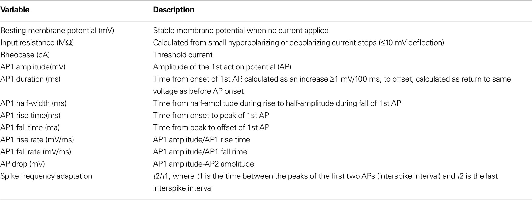
Table 1. Electrophysiological variables. Action potential properties measured from response to twice threshold, 500-ms current injection from first action potential (AP1) and second action potential (AP2). AP2 variables not listed as the same measurements were made for AP2 as listed for AP1.
Histological procedure
Neurons were filled with biocytin by a patch pipette. The slices were kept overnight in 4% paraformaldehyde in 0.1 M phosphate buffer (PB) at 4ºC. The slices were then rinsed three times for 5 min per rinse on a shaker in 0.1 M PB. They were placed in 30% sucrose mixture (30 g sucrose dissolved in 50 ml ddH20 and 50 ml 0.24 M PB per 100 ml) for 2 h and then frozen on dry ice in tissue freezing medium. The slices were kept overnight in a −80ºC freezer. The slices were defrosted and the tissue freezing medium was removed by three 20-min rinses in 0.1 M PB while on a shaker. The slices were kept in 1% hydrogen peroxide in 0.1 M PB for 30 min on the shaker to pretreat the tissue, then were rinsed twice in 0.02 M potassium phosphate saline (KPBS) for 20 min on the shaker. The slices were then kept overnight on the shaker in Avidin-Biotin-Peroxidase Complex. The slices were then rinsed three times in 0.02 M KPBS for 20 min each on the shaker. Each slice was then placed in DAB (0.7 mg/ml 3,3′-diaminobenzidine, 0.2 mg/ml urea hydrogen peroxide, 0.0 6M Tris buffer in 0.02 M KPBS) until the slice turned light brown then immediately transferred to 0.02 M KPBS and transferred again to fresh 0.02 M KPBS after a few minutes. The stained slices were rinsed a final time in 0.02 M KPBS for 20 min on a shaker. Each slice was observed under a light microscope and then mounted onto a slide using crystal mount.
Reconstruction and analysis of morphology
Successfully filled and stained neurons were then reconstructed using Neurolucida software (MicroBrightField). The neurons were viewed with 100× oil objective on an Olympus IX71 inverted light microscope or an Olympus BX51 upright light microscope. The Neurolucida program projects the microscope image onto a computer drawing tablet. The neuron’s processes were traced manually while the program recorded the coordinates of the tracing to create a digital three dimensional reconstruction. The x and y axis form the horizontal plane of the slice, while the z axis is the depth. The user defined an initial reference point for each tracing. The z coordinate was then determined by adjustment of the focus. In addition to the neuron, the pia and white matter were drawn.
The Neurolucida Explorer program was used to measure 67 morphological variables of the reconstruction. See Table 2 for descriptions.
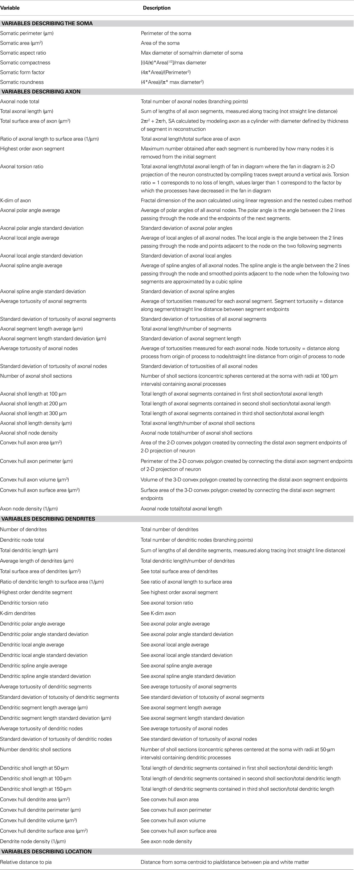
Table 2. Morphological variables. Variables were extracted using the Neurolucida Explorer program by MicroBrightField.
Shrinkage percentage in the z-axis was on average 48.97 ± 1.95%. No shrinkage correction was applied.
Principal component analysis and cluster analysis
The dataset of neurons could now be represented as a matrix, with each row corresponding to a neuron and each column corresponding to a variable. The data was then standardized, where the standardized values of each variable are computed as the difference between the actual value and the mean divided by the standard deviation. PCA reduces the dimensionality of the dataset, while preserving as much of the variance as possible by mapping the coordinate system defined by the old variables to a new lower dimensional coordinate system defined by principal components that are orthogonal, thus uncorrelated, linear combinations of the original variables. As many of the original variables are related, the principal components produced by PCA reduce this redundancy. By PCA, a new space is generated onto which the dataset can be projected and classified by cluster analysis.
The principal components were calculated using the factor analysis function in STATISTICA (StatSoft). The principal components are found by an eigenvalue decomposition of the correlation matrix of the standardized data. The eigenvectors of the correlation matrix are the principal components (PCs) and the corresponding eigenvalues give the variance preserved by each principal component. The number of PCs maintaining a significant amount of variance will always be less than the number of original variables, which is why PCA reduces the dimensionality of the dataset (Jambu, 1991 ).
Several criteria were used to decide how many principal components to retain for cluster analysis. First, only principal components with eigenvalues greater than one are considered. The original variables have an eigenvalue of one, as the data is standardized, thus any principal component with an eigenvalue greater than one describes more of the data’s variance than an original variable. Second, the “scree test” was used (Cattell, 1966 ). A plot of the eigenvalues of the principal components is examined for when the decrease in eigenvalue plateaus. In all cases either 2 or 3 principal components were retained.
Cluster Analysis is then performed on each dataset in the principal component vector space using Clustan (Clustan Ltd.). Hierarchical clustering using Euclidean distance squared as the multi- dimensional distance metric and Ward’s method as the linkage rule was performed. Ward’s method minimizes the distance squared between any two clusters that can be formed at each step of clustering (Ward, 1963 ). Alternatively, cluster analysis was performed on the standardized data before PCA. The results obtained from this method did not dramatically differ from the results obtained with PCA. The only differences were reordering of cells within clusters and movement of cells between neighboring clusters contained in Group 1.
Statistical analysis of clusters
Three statistical tests were done to find the clustering levels which have significance at the 5% level. The Best Cut Test does an analysis of variance on the fusion values (distance at which two clusters join) at every level in the dendrogram. The realized deviates, defined as the standardized difference between a fusion value and the mean fusion value, are compared to find significantly large realized deviates. A large realized deviate is significant if the fusion value is at least 1.96 standard deviations from the mean. The upper tail test applies the upper tailed t-test to the fusion values using t-statistic of realized deviate*(n-1) over n-2 degrees of freedom to find the significant increases in fusion value. The bootstrap test performs 1000 trials of randomizing the data, cluster analysis on the randomized data and then compares the random trees to the actual tree. The data matrix was randomized by randomly permuting the order of entries in each column independently. This scrambles the values of each variable for a given cell, thus disturbing any correlations between variables for each cell, but not changing the distribution of values for each variable. The random trees were compared to the actual tree by plotting fusion value vs. number of clusters for the actual data and the distribution of the randomized data with a confidence interval of 1 standard deviation around the mean. Significant departures of the actual fusion values from random, determined by the t-statistic, indicate a number of clusters that are statistically significant. The first level at which significance was found by all three tests is the partition used (indicated in Figures 1 A, 2 A and 3 C–E by bracketing on the bottom of the dendrogram and cut-off linkage distance by a horizontal line).
Finally, in the morphological or physiological clustering we did not detect any obvious bias towards the individual patching the cell, individual reconstructing the cell, or age of the mouse.

Figure 1. Anatomical classification of SOM neurons. (A) Ward’s method of hierarchical unsupervised clustering based on 67 morphological variables applied to 39 SOM positive interneurons. The first 2 principal components were retained for cluster analysis. The x-axis of dendrogram shows individual cells and the y-axis represents the linkage distance measured by the Euclidean distance squared. Open circles indicate the centroid cell of each cluster. Black brackets outline the clusters statistically significant at the 5% level and a horizontal line indicates this cut-off linkage distance. The groups discussed in the text are colored: group 1 in purple, group 2 in orange and group 3 in green. (B) Scatterplot of dataset in principal component space. The x-axis represents the first principal component (PC1) and the y-axis represents the second principal component (PC2). Centroids of clusters are labeled and circled in red. Orthogonal lines separating the three groups are shown. (C) Neurolucida reconstructions of representative cells of each cluster. Axons are shown in blue and dendrites in red.
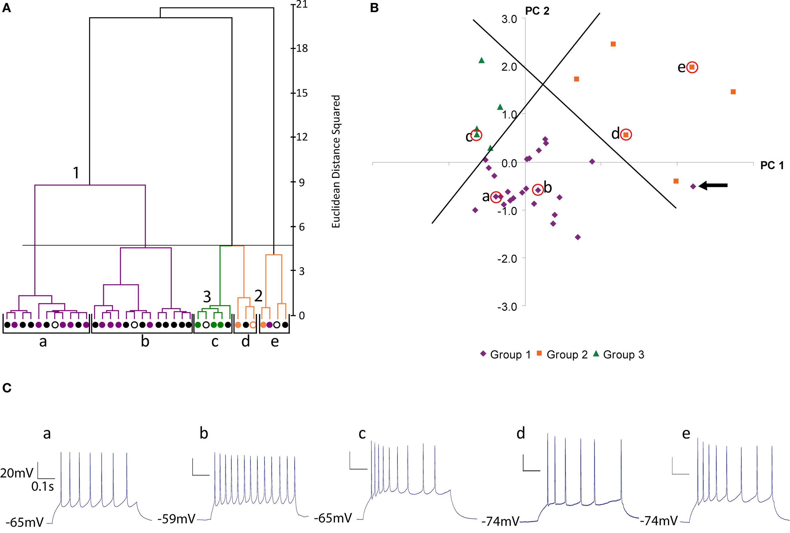
Figure 2. Physiological classification of SOM neurons. (A) Ward’s method of hierarchical unsupervised clustering based on 19 electrophysiological variables applied to 36 SOM positive interneurons. The first 2 principal components were retained for cluster analysis. The x-axis of dendrogram shows individual cells and the y-axis represents the linkage distance measured by Euclidean distance squared. Open circles indicate the centroid cell of each cluster. Black brackets outline the clusters statistically significant at the 5% level and a horizontal line indicates this cut-off linkage distance. Group 1 (Martinotti cells) are shown in purple, group 2 in orange and group 3 in green. This color scheme is based on the clustering by morphological variables (See Figure 1 ) and will be preserved for all figures. Black cells are those without morphological reconstruction. (B) Scatterplot of dataset in principal component space. The x-axis represents the first principal component (PC1) and the y-axis represents the second principal component. Centroids of clusters are labeled and circled in red. Orthogonal lines separating the three groups are shown. The outlier in cluster e is indicated with an arrow. (PC2). (C) Current clamp recording of response to twice threshold current pulse for the centroid cells of each cluster.
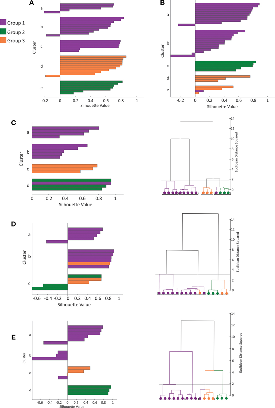
Figure 3. Silhouette analysis. (A) Plot of silhouette values for clustering of 39 cells by morphological variables (see Figure 1 A for dendrogram of this dataset). On the y-axis cells in each cluster are ordered by decreasing silhouette value. The silhouette value can range between −1 and 1. Large positive values indicate clusters are distinct with greater intra-cluster similarity than between cluster similarity (See Materials and Methods for further explanation). The x-axis represents the silhouette value (See Materials and Methods). (B) Plot of silhouette values for clustering of 36 cells by electrophysiolgical variables (see Figure 2 A for dendrogram of this dataset). (C–E) Plot of silhouette values (left) and dendrogram (right) for clustering of the 16 cells with both recordings and reconstructions by morphological variables (C), by electrophysiological variables (D) and by electrophysiological and morphological variables (E). The first 2 principal components were retained for cluster analysis by the morphology variables (C) and electrophysiological variables (D). The first 3 principal components were retained for cluster analysis by both the electrophysiology and morphology variables (E). Again the color scheme is based on the clustering by morphology (see Figure 1 ).
K-means clustering
K-means clustering was performed for each dataset using Clustan’s Focal Point clustering algorithm, with K equal to the number of significant clusters from hierarchical clustering. Focal Point runs the K-means algorithm several times with different initial case orders, which is an important permutation as the K-means algorithm is sensitive to case order. It ranks these solutions based on the minimization of Euclidean distance squared.
Silhouette Analysis
Silhouette analysis measures the quality of the clustering by examining the within cluster distances and between cluster distances (Rousseeuw, 1987 ). The silhouette value of a data point i in cluster A is
s(i) = (b(i)−a(i))/max[a(i),b(i)]
where a(i) is the average Euclidean distance between i and all other datapoint in cluster A, b(i) is the smallest average Euclidean distance between i and all datapoints in any other clusters (the average Euclidean distance between i and all datapoints in cluster B, the nearest neighbor to cluster A). The value of s(i) is between −1 and 1. The silhouette width of a clustering is defined as the average of s(i) for all datapoints. Large positive values indicate that the cluster is compact and distinct from other clusters. In addition to calculation of the silhouette width of each clustering, the silhouette width of randomized clustering for each dataset was calculated. The data was randomized as described above for the bootstrap test. The same procedure for cluster analysis was performed on 500 randomized matrices of each dataset and the silhouette width of each clustering was computed. S(random) is the average of the 500 silhouette widths.
Statistical analysis of variables
To determine which variables are important in distinguishing between the groups identified by cluster analysis, the group mean and standard error was calculated for every variable and the groups were compared for significant differences (Mann Whitney U Test). Additionally, the correlation between the PCs and the original variables was calculated as another measure of which variables are discriminating. Variables highly correlated with the principal components used for cluster analysis are more discriminating. Most of the variables with significant differences between the groups were highly correlated with the PCs (Tables 6 and 7 )
Results
Morphological Classification of Subtypes of Somatostatin Interneurons
To identify subtypes of SOM-positive neurons, morphology and electrophysiology were quantitatively characterized. GFP-positive neurons were patched, recorded from in current clamp mode, filled with biocytin and processed for morphological analysis. 19 electrophysiological variables were measured from current clamp recordings. In addition, 67 morphological variables describing the soma, dendrites, axon and somatic location (relative to the pial surface) were measured from the Neurolucida reconstructions of the patched cells. From a dataset of 59 SOM-positive interneurons from mouse primary somatosensory, visual and frontal cortex, 39 cells had complete reconstructions, 36 cells had high quality electrophysiological recordings, and 16 cells had both complete reconstructions and recordings.
We first explored the statistical structure of the morphological dataset. Cluster analysis using morphological variables was performed with the 39 cells with complete reconstructions, and it revealed five clusters of neurons, grouped into three major branches (Figure 1 A, labeled purple, orange and green). One major group encompassed approximately half of the neurons, and could be subdivided into three clusters (purple cells, clusters a, b and c), and was separated by a large Euclidian distance from the other two clusters (orange-d and green-e). In addition, clusters showed no bias with respect to age of the mouse, cortical area, individual patching the cell, or individual reconstructing the cell (not shown).
We further explored the morphological variability of the neurons by plotting their position in principal component space, using the first two principal components as Cartesian axes (Figure 1 B). In this analysis one seeks to draw lines that separate each group in a different section of the graph. In this PCA space, the first major group of the cluster analysis (purple cells, corresponding to clusters a, b and c) was clearly separated from the other two branches (orange-cluster d and green-cluster e cells). Within this first group (purple cells), no clear subgroups were observed in PCA space. Clusters d (orange) and e (green) were separated from each other by a second line, with one exception (orange neuron on top). Because of these results in PCA space, although the morphological grouping was significant at the 5 cluster level (black brackets in Figure 1 A; see Materials and Method and Statistical Validation section below), we chose to group the data into three classes (named groups 1, 2 and 3, and colored purple, orange and green, for the rest of the study).
Examining the morphologies of the cells revealed that group 1 (n = 21) corresponded to morphologies traditionally associated with Martinotti cells, a well-characterized subtype of SOM interneurons (Wahle, 1993 ; Kawaguchi and Kubota, 1996 ; De Felipe, 2002 ; Wang et al., 2004 ). Martinotti cells are found in layers 2/3, 5 and 6 and have a characteristic ascending axon that sends several collaterals to layer 2/3 and layer 1. The axon branches extensively in these layers, particularly in layer 1 where the collaterals branch horizontally, for distances as long as 400 µm (see Figure 1 C, for representative examples; Figure S1A in Supplementary Material, for all neurons)
On the other hand, group 2 (n = 11) and 3 (n = 7) neurons were quite distinct from Martinotti cells, with very different axonal morphologies. In group 2 and 3 cells, the axon ascended in a very direct course with minimal branching and, in most cases, did not enter layer 1 (Figure 1 C and Figures S1 B,C in Supplementary Material). Axons generally had only one main ascending collateral, or at most, two or three. Initially, we interpreted this sparse axon as a filling or reconstruction artifact, but closer examination of the cells found no evidence of incomplete staining or cut processes. Indeed, endings of their axonal processes did not taper and had apparently normal terminations in the middle of the section (see below). Moreover, group 2 and 3 neurons all had healthy-looking dendrites, without beading, with group 2 cells displaying multipolar morphology and group 3 cells bipolar morphology. Group 2 and 3 cells were found in layers 2/3, 4 and 5.
The combined cluster/PCA analysis indicated that the morphological variance of our database of neurons could be well captured by the hypothesis that they belonged to three major subtypes of cells.
Physiological Classification of Subtypes of Somatostatin Interneurons
We then sought to use the electrophysiological database to test whether the groups defined by the morphological variables were correlated to electrophysiological groups. For this analysis we used neurons with complete physiological data, regardless of their anatomical reconstruction. Therefore, the two datasets, anatomical and physiological, were not identical but partly overlapped.
When the 36 cells with recordings were clustered by electrophysiology variables, we found significant grouping at the 5 cluster level, by several independent statistical tests (Figure 2 A; black brackets; clusters a to e, all neurons with reconstructions colored according to morphological groups described above). The first two clusters (a and b) constituted a group (group 1, purple), in which, remarkably, all of its reconstructed neurons had been previously identified as belonging to the group 1 from the morphological clustering (Figure 1 A, purple cells). Besides this first group, the remaining 3 clusters (c–e) contain all neurons previously identified as belonging to the morphological groups 2 and 3 and, moreover, separated these cells in good agreement with these 2 groups. More specifically, physiological cluster c corresponded to morphological group 3 (green) and physiological clusters d and e correspond to morphological group 2 (orange) with one outlier neuron in cluster e that belonged to the first morphological group (purple).
In addition to the cluster analysis, we again explored the statistical structure of the physiological data by plotting the dataset in principal component space (Figure 2 B). This PCA analysis revealed a less compact grouping than the morphological dataset. Nevertheless, with two orthogonal lines, one could clearly separate neurons belonging to groups 1, 2 and 3, again, with only one exception, the previously mentioned outlier neuron from cluster e (Figure 2 B, purple neuron indicated by arrow). This neuron, interestingly, was close in PCA space to the border between groups 1 and 2.
Inspection of the physiological responses of these three groups of neurons was in agreement with the statistical clustering. Group 1 cells (n = 24) displayed a regular spiking firing pattern, non-stuttering and non-fast spiking, with varying degrees of spike frequency adaptation from small to moderate increases in interspike interval (Figure 2 C, a and b; average spike frequency adaptation 1.674 ± 0.092; see Ascoli et al., 2008 for definition of electrophysiological variables according to the Petilla nomenclature). For the majority of neurons the action potential (AP) amplitude decayed only slightly over the course of a train (average AP drop 2.619 ± 0.479 mV). Group 1 cells also tended to have a lower rheobase (36.042 ± 6.363 pA) than group 2 or 3 cells (49.286 ± 10.025 pA and 55.000 ± 12.845 pA, respectively) and a significantly more depolarized resting membrane potential (Table 3 ). On the other hand, group 2 cells (n = 7) displayed both regular spiking and stuttering firing patterns. There was a greater spike frequency adaptation (2.244 ± 0.385) and amplitude accommodation than group 1 cells. Group 3 cells (n = 5) were regular spiking, with a degree of frequency adaptation similar to group 2 cells (2.657 ± 0.493) and significantly narrower action potentials (Table 3 , AP1 half-width, AP2 half-width). One cell (cell 3, see Figure S2 in Supplementary Material) had an unusual early offset firing pattern of only three to four action potentials per train, and then was silent at a depolarized membrane potential for the remainder of the current pulse. Of the four other group 3 cells, three showed marked amplitude drops in the first few spikes and the other showed amplitude accommodation similar to group 2 cells (Figure S2).
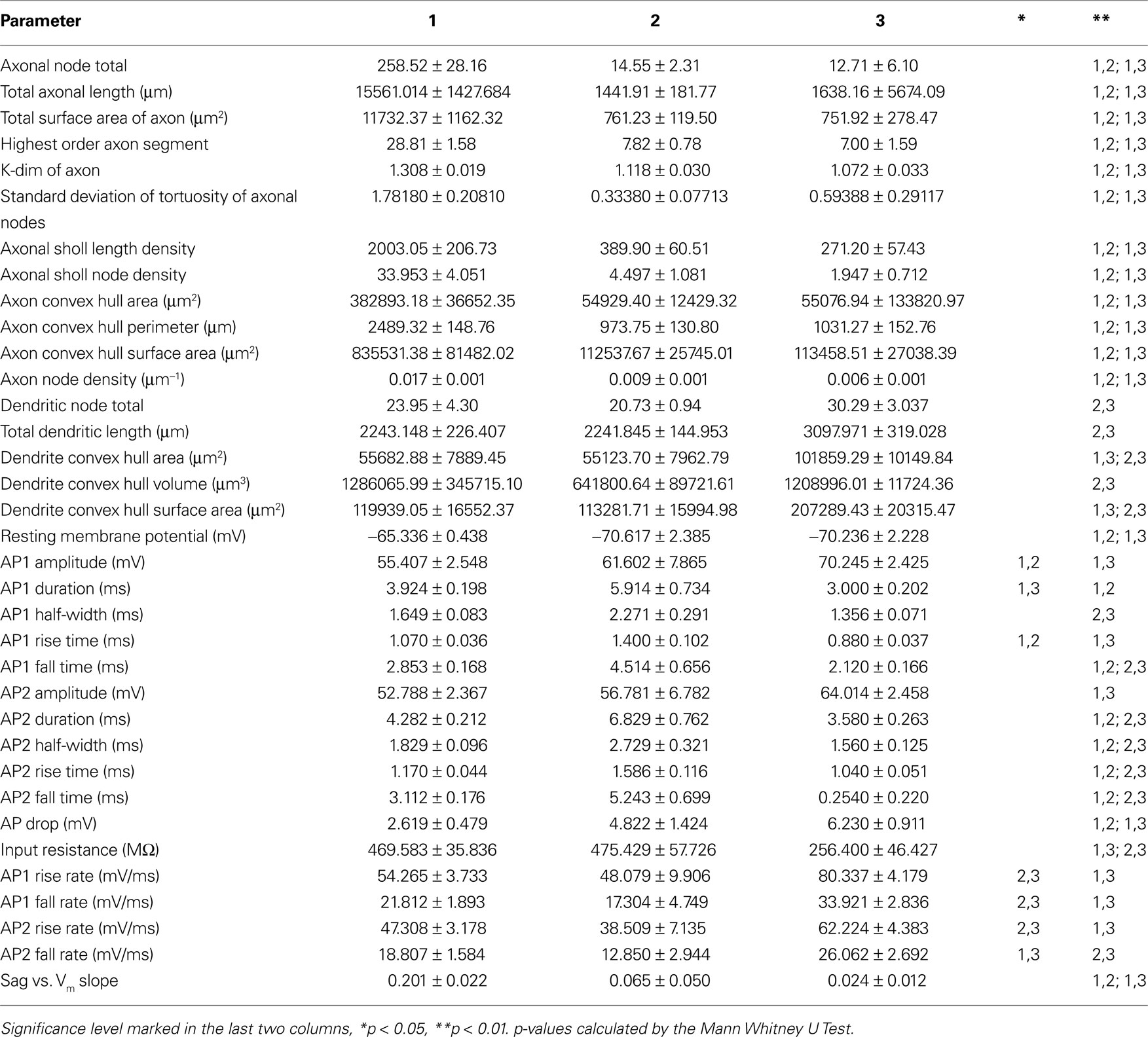
Table 3. Average values ± standard error for the morphological and electrophysiological variables with significant differences between groups.
The joint interpretation of the morphological and physiological clustering and PCA analysis was consistent with a simple model of three basic subgroups of SOM neurons. Group 1 is clear: it is composed of Martinotti cells and is clearly delineated in the morphological and physiological clustering dendrograms. Group 2 and group 3 are also distinct in both morphological and physiological clustering, although they are closer to each other in statistical space. Specifically, the close proximity and some overlap between groups 2 and 3 in the principal component space of the morphology dataset versus their complete separation in the principal component space of the electrophysiology dataset suggests that groups 2 and 3 have morphological similarities, although they are physiologically quite different. One could further subdivide the morphological group 1 into three different subgroups (a, b, c; based on the morphological clustering), or the physiological group 3 into 2 subgroups (d and e; based on the electrophysiological clustering). Nevertheless, for simplicity, for the rest of the study we followed the basic three groups (1, 2 and 3), first apparent from the morphological clustering.
These results display a remarkably good agreement between the morphological and physiological classifications, which because they are based on completely independent datasets, confirm each other. In fact, with this basic classification into three groups every neuron is classified into the same groups in both morphological and physiological analysis, with one exception, the outlier purple cell that clusters with group 3 in the physiology, but which is actually borderline in PCA space. Given the tight correlation between morphological group and electrophysiological group for the 16 cells that are in both morphology and electrophysiology datasets, we propose that morphological groups 1, 2 and 3 correspond to electrophysiological groups 1, 2, 3. We do recognize that for a cell belonging to only one of the datasets it is possible that it does not belong to the corresponding group of the other dataset. However, we find this unlikely given that for 15/16 cells the correspondence between morphological and electrophysiological groups was accurate.
Statistical Validation of Clusters
We then explored how robust the classification based on cluster analysis actually was, using a variety of statistical analyses. We first used three tests (best cut, upper tail and bootstrap) that are routinely applied to test whether the dataset has a non-uniform structure, an important validation as cluster analysis will always return a clustering tree, regardless of the distribution of the data. Specifically, the best cut test distinguishes the clustering profile of a dataset containing groups from the profile of a dataset with a continuum of points by analyzing the fusion values. Cluster analysis performed on a dataset not containing groups would return arbitrary divisions and thus the fusion values would be continuous, with no large jumps. However, if the dataset does contain groups then at the partitions between the groups large fusion values should be seen. The best cut test finds if there is a linkage cut-off distance at which this fusion value profile occurs. The upper tail test also locates significantly large fusion values. The bootstrap test determines the linkage distance at which the results significantly deviate from random. Indeed, using these three tests, the clusters (as marked by brackets in Figures 1 A and 2 A) were found to be statistically significant at 5% level (See Materials and Methods for details). Thus, three independent significance tests all show that the dataset does have a non-uniform structure, and thus could be classified into meaningful clusters.
Following this, we sought to confirm whether the hierarchical classification using Ward’s method was reliable, using K-means clustering with K specified as the number of significant clusters from hierarchical clustering. K-means clustering is a top-down clustering method, in contrast to hierarchical clustering which is a bottom-up method. (MacQueen, 1967 ). While hierarchical classification is inflexible in that cells initially linked stay linked, resulting in a sometimes local optimization rather than global optimization, K-means can reassign cells at a later stage of clustering if it will result in a better optimization. Indeed, the reliability of Ward’s method hierarchical clustering for this dataset was proven by the agreement between the two methods (Table 4 ). Only a small percentage of cells switched clusters and always stayed within the same group, for example in the 39 morphology cluster cell 27 switched from cluster a to cluster b, both of which are included in Group 1 (Table S3 in Supplementary Material). Such stability between two different algorithms demonstrates that the groups are robust.
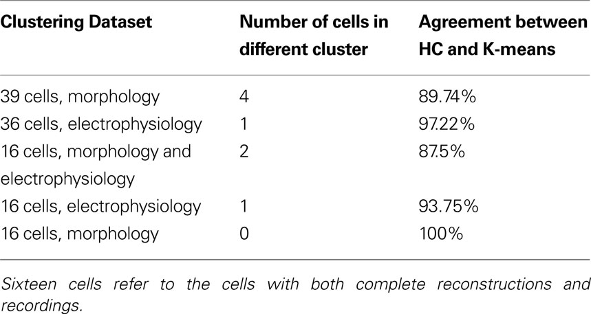
Table 4. Agreement of hierarchical clustering (HC) using Ward’s method with K-means clustering for K = number of clusters determined significant by HC.
In addition, to assess the quality of the hierarchical clusters obtained by Ward’s method, we computed the silhouette width of each clustering (Figures 3 A,B) (Rousseeuw, 1987 , See Materials and Methods). Silhouette width is a measure of the appropriateness of each assignment of a datapoint to a cluster. A silhouette width around 0 indicates the datapoint is intermediate between two clusters, silhouette width close to 1 indicates that the point is well assigned and a silhouette width close to –1 indicates that the point is poorly assigned. Constructing a plot of silhouette widths helps reveal the structure of the dataset, and thus to identify natural groups from artificially imposed groups. Using this analysis, we found that the silhouette widths of the clustering by morphology and clustering by electrophysiology confirmed that a natural structure has been found. Such a silhouette width indicates that the distances within clusters are small in comparison to the distances between clusters. Thus, the dataset has a structure containing discrete and compact clusters with clear separation between clusters. In fact, visually inspecting the silhouette plot for each cluster revealed that the majority of cells are well classified.
As a final additional measure of statistical significance, the silhouette width was computed for 500 trials of randomized data, following the same clustering procedure (Table 5 ). The average silhouette widths for these randomized trials was drastically lower than for the actual datasets, again demonstrating that the datasets have a strong structure which was disrupted by the randomization.
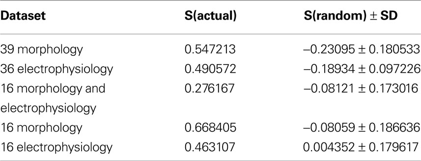
Table 5. Comparison of silhouette widths of each dataset to the mean silhouette width of 500 trials of clustering randomized data.
Quality of Clustering Combining Different Groups of Variables
To determine the quality of classification based on electrophysiological variables, morphological variables and all variables combined, we performed a separate analysis of the 16 cells with both complete reconstructions and recordings (Figures 3 C–E). This dataset was used to control for differences in sample size and non-overlapping data points between the 36 cell electrophysiology and 39 cell morphology datasets. The clusters found by morphology only, electrophysiology only and both morphology and electrophysiology were in good agreement with the three groups previously identified. Each set of variables had one outlier in the clustering therefore clustering using the combined sets of variables was not an entirely better method. Judging the strength of structure of the three datasets by silhouette width revealed that the clustering by morphological variables has the strongest structure, by electrophysiological variables the next strongest, and by all variables the weakest. The low silhouette width of the combined morphological and electrophysiological variables dataset could be due to the strong correlations within clusters between morphological variables and between electrophysiological variables. With all variables combined, the clusters had a less compact shape due to the multimodality of variables. Thus when clustering by electrophysiology variables only or morphological variables only can discriminate between groups as in our case, we found no particular advantage to clustering by morphological and electrophysiological variables combined.
Morphological Characteristics Defining SOM Subgroups
After establishing the reliability and validity of the classification based on three major groups of SOM interneurons, we explored more carefully the physiological and morphological characteristics of each of them. First, we concentrated on the analysis of the morphological variables that were statistical predictors of each of the three subtypes of neurons (Table 3 ). Morphologically, the axon was the most important feature in discriminating between the group 1 and groups 2 and 3, as can be seen by direct inspection of the morphologies. Group 1 cells had typical Martinotti cell axons that extend through layers above the soma and branch extensively, particularly at the pial surface and in the home layer. Group 2 and 3 cells also had an ascending axon, but their axons were much sparser and were contained within a narrow vertical column. Statistically, Group 1 cells had principal component 1 (PC1) values distinct from groups 2 and 3 (Figure 1 B) and, indeed, the first principal component of the dataset is highly correlated with 12 axon variables (Table 6 ). Six of these variables, axonal node total, total axonal length, total surface area of axon, convex hull axon area, convex hull axon perimeter and convex hull axon surface area, describe the size of the axon in both two and three dimensions. The other variables, i.e. highest order axon segment, axonal Sholl length and node densities and axonal node density describe the degree of axon branching and k-dim axon describes the dimensionality of the axon. Given these correlations PC 1 can be interpreted as a measure of axon size and complexity. Accordingly, there were significant differences for several parameters describing the size, shape and dimensionality of the axon between groups 2 and 3 and group 1 (Table 3 ).
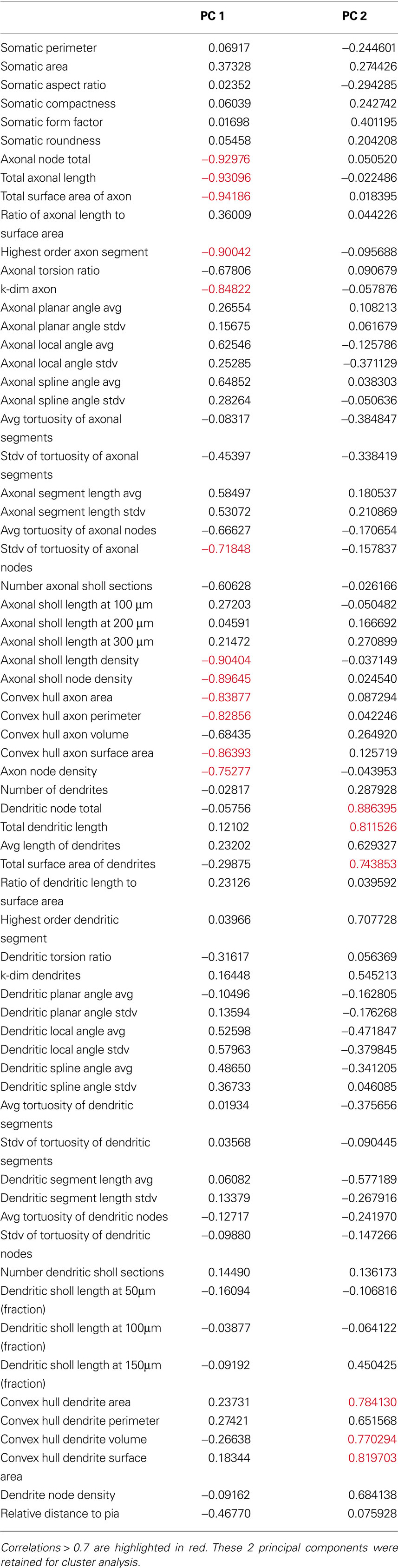
Table 6. Correlations between morphological variables and the first 2 principal components of the 39-cells morphology variables dataset.
The layers targeted by the axon also differed between group 1 and groups 2 and 3. Group 1 cells extensively branched in layer 1, where Martinotti cells are known to synapse on the apical dendrite tufts of pyramidal cells (Wang et al., 2004 ; Silberberg and Markram, 2007 ). In contrast, 13 of the 18 group 2 and 3 cells (72.2%) had axons that avoided layer 1. Some had axons that suddenly terminated at layer 1, while others made an abrupt turn at the layer 1 border and either hooked or continue tangentially along the border (Figure 4 A). Interestingly, there was a striking direction preference of this bend at the layer 1 border; in every single case axons turned medially in the slice. Examination of the axons of these cells showed axonal boutons in layer 2/3 (Figure 4 B). As mentioned, these axons did not taper and were not cut, terminating in an apparently normal fashion, away from the sectioned surface of the slice (Figure S3B in Supplementary Material). In contrast, the termination of cut axons had larger, more roundly swollen ends and darker ends, and always ended at the very edge of the slice (Figure S3C in Supplementary Material).
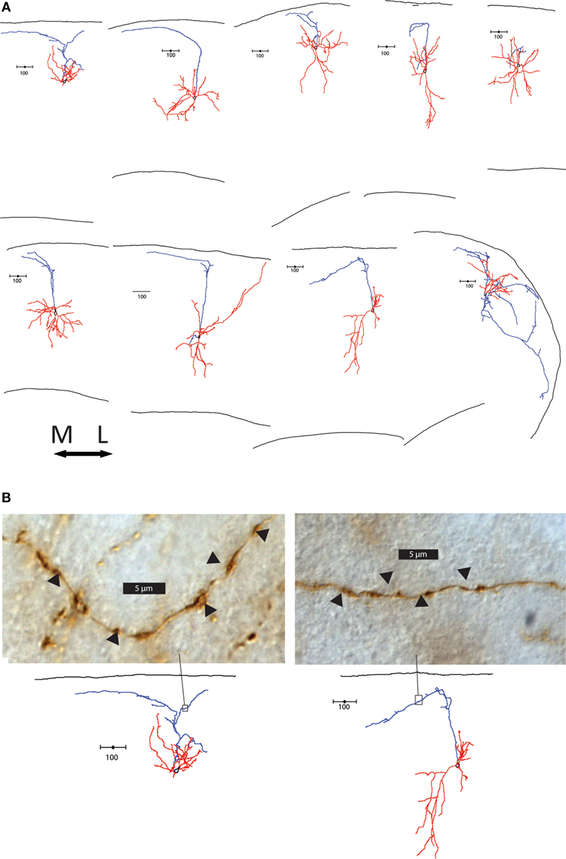
Figure 4. Axonal features of group 2 and 3 cells. (A) Axons of group 2 and 3 cells avoid layer 1. The 9 cells with axons that turn or hook are shown, all oriented with respect to the medial-lateral axis above. Note the preference of direction medially. (B) Light microscope images of section of two cells’ axons in the area boxed in the reconstructions below. Swellings in the axon indicated by arrow heads are possible boutons, found along the axons in layer 2/3.
The size and shape of the dendritic arbor anatomically distinguished groups 2 and 3, which had overall similar axon morphology. While group 1 was separated from groups 2 and 3 on the PC1 axis, groups 2 and 3 were separated from each other on the PC2 axis (Figure 1 B). Examining correlations between the original variables and PC2, revealed that PC2 was highly correlated with several dendrite variables describing the size of the dendrites in two and three dimensions (Table 6 ). This possibility is supported by significant differences between the two groups for several variables describing size of the dendritic processes (Table 3 ). Group 3 cells had the largest dendritic arbor of the three groups, while group 2 cells had the smallest dendritic arbor, by measures of length and convex hull size. Additionally, group 3 cells had bitufted dendrites, while group 2 cells have multipolar dendrites (Figure S1 in Supplementary Material). Group 1 dendrites were varied, with some multipolar, while others show a preference for extending only upward or downward.
Electrophysiological Characteristics Defining SOM Subgroups
We then focused on the electrophysiological parameters, analyzing both passive and active physiological properties, such as resting membrane state and firing pattern (Table 2 , Figure 5 ). There were significant differences among the passive properties of the three groups (Figure 5 A). Group 2 and 3 cells were significantly (p < 0.025) more hyperpolarized at rest (−70.617 ± 2.385 mV and −70.236 ± 2.228 mV respectively) than Group 1 cells (−65.336 ± 0.438 mV). Group 3 cells had significantly (p < 0.025) lower input resistance (256.400 ± 46.427 MΩ) than both group 1 and 2 cells (469.583 ± 35.836 MΩ and 475.429 ± 57.726 MΩ respectively). In response to hyperpolarizing current, only group 1 cells consistently demonstrated a sag response. This variable was not used for clustering as only 32 of the 36 cells (23 of 24 group 1, 5 of 7 group 2 and 4 of 5 group 3 cells) were given a series of hyperpolarizing current steps. The slope of the regression line fitted to the sag vs. membrane potential was used as the variable for comparison, with sag defined as the difference between the most negative membrane potential during a 1s hyperpolarizing current step and the steady membrane potential in the last 100ms of the step. Group 1 significantly differed (p < 0.005 and p < 0.01 respectively) from groups 2 and 3 (Table 3 ). Some cells showed a depolarized rebound after the hyperpolarizing step, but only one cell in group 1 spiked as a result of the rebound depolarization. As Martinotti cells are known to display a sag response, these results further support that groups 2 and 3 are distinct from Martinotti cells.
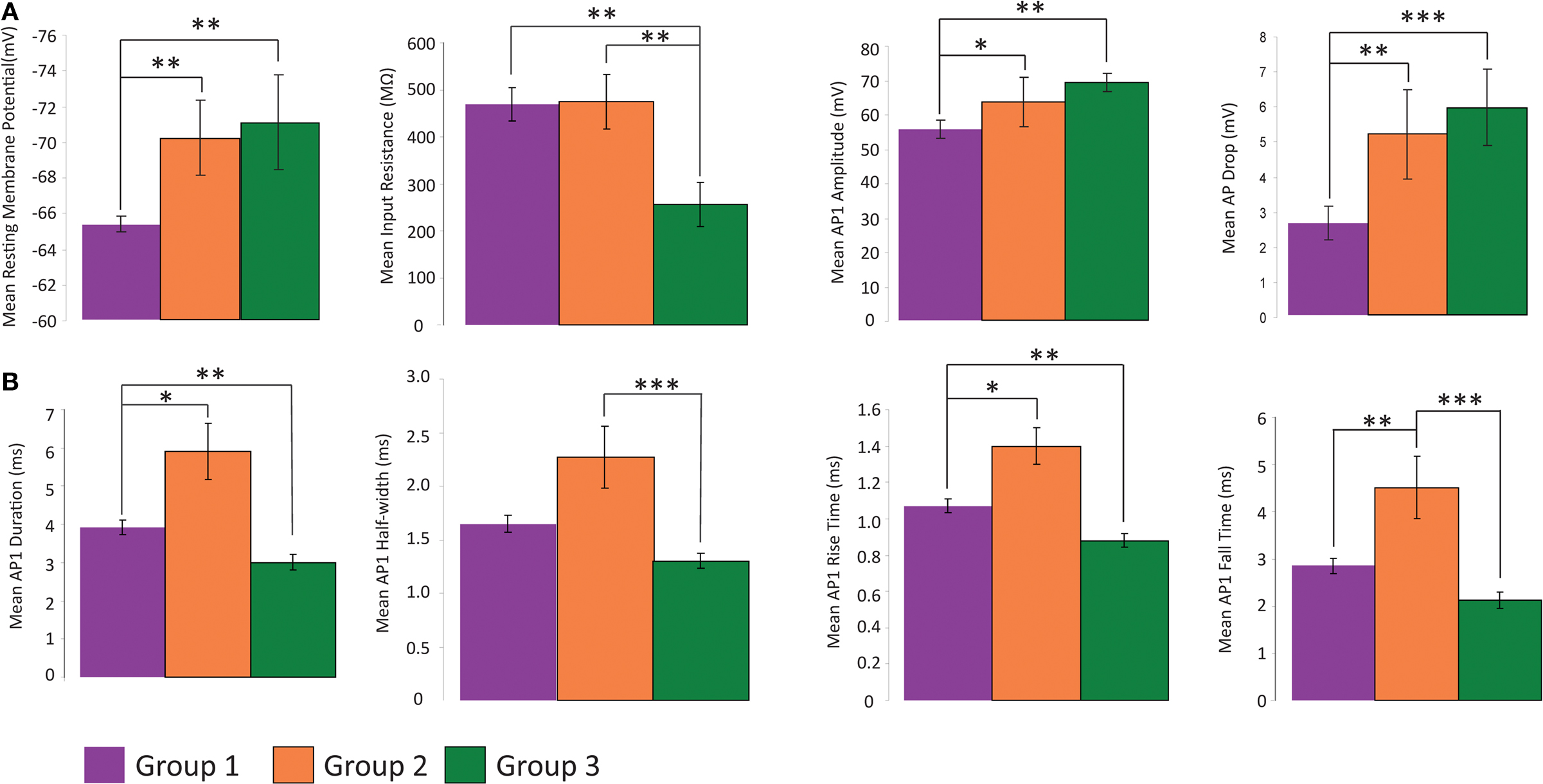
Figure 5. Analysis of electrophysiology variables. Comparison of physiological variables that distinguish the three groups with regards to several variables. All data shown mean ± standard error (A) Groups 2 and 3 are distinct from group 1 with respect to RMP, input resistance, AP amplitude and difference in amplitude between first and second AP of a train. (B) Each group has a distinct time course of AP, with group 1 intermediate between groups 2 and 3. (*p ≤ 0.05, **p ≤ 0.025, ***p ≤ 0.005, Mann Whitney U Test)
We found that the first principal component was highly correlated with the variables measuring the duration, half-width, rise time and fall time of AP1 and AP2 (Table 7 ). Therefore it is not surprising that these variables distinguished all three groups (Figure 5 B). Specifically, the groups had distinct AP duration, with the values of group 1 (AP1 duration 3.924 ± 0.198 ms) being intermediate between groups 3 (AP1 duration 3.000 ± 0.202 ms, p < 0.05) and 2 (AP1 duration 5.914 ± 0.734 ms, p < 0.025). In addition, groups 1 and 3 both had faster half-width (AP1 half-width 1.649 ± 0.083 ms and p < 0.005, 1.356 ± 0.071 ms respectively) rise time (AP1 rise time p < 0.025, 1.070 ± 0.036 ms and p < 0.005 0.880 ± 0.037 respectively), and fall time (AP1 fall time p < 0.025, 2.853 ± 0.168 ms and p < 0.005, 2.120 ± 0.166 ms respectively) than group 2 (AP1 half width 2.271 ± 0.291 ms, AP1 rise time 1.400 ± 0.102 ms and AP1 fall time 4.514 ± 0.656 ms) while groups 1 and 2 had significantly slower (p < 0.025) rise rates (AP1 rise rate 54.265 ± 3.733 mV/ms and 48.079 ± 9.906 mV/ms respectively) and fall rates (AP1 fall rate 21.812 ± 1.891 mV/ms and 17.304 ± 4.749 mV/ms respectively) than group 3 (AP1 rise rate 80.337 ± 4.179 mV/ms, AP1 fall rate 33.921 ± 2.836 mV/ms). The slower rise and fall rate of group 1 was more likely due to group 1 having smaller AP amplitude, while the difference in rise and fall rate between group 2 and 3 resulted from the difference in AP rise and fall time.
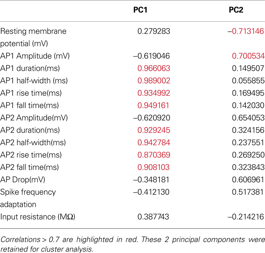
Table 7. Correlations between electrophysiological variables and the first 2 principal components of the 36-cells electrophysiology variables dataset.
In addition, all three groups showed spike frequency adaptation, with group 2 and 3 cells showing a greater degree of adaptation (spike frequency adaptation values group 1: 1.674 ± 0.092, group 2: 2.244 ± 0.385, group 3: 2.657 ± 0.493). Group 2 and 3 cells had greater action potential amplitude as measured from the first two action potentials in a train elicited by twice threshold current injection (AP1 amplitude p < 0.05, 61.602 ± 7.865 mV and p < 0.025, 70.245 ± 2.425 mV respectively) than group 1 (AP1 amplitude 55.407 ± 2.548 mV) and also had a significantly larger (p < 0.025, p < 5 × 10⁻³) drop in amplitude between these first two action potentials (AP drop 4.822 ± 1.424 mV and 6.230 ± 0.911 mV respectively) than Group 1 (AP drop 2.619 ± 0.479 mV; Figure 4 A, Table 3 ).
Most cells were regular spiking, but three group 2 cells (75, 76, 77) were stuttering, defined as the firing of groups of action potentials that are interrupted by silent periods of varying length (Markram et al., 2004 ; Ascoli et al., 2008 ). With only an 8.3% incidence of stuttering cells in the dataset, this is too low a number to conclude that all stuttering cells are group 2 cells, but does indicate that stuttering is a distinctive firing pattern of some group 2 cells. It can additionally be noted that group 2 cells had greater variability in firing patterns, by plotting the dataset in the PC1–PC2 plane (Figure 2 B). Groups 1 and 3 were restricted to a much smaller region of the PC1 values, than are Group 2 cells indicating that Group 2 cells have a larger and separate range of values for those variables correlated with PC1 (AP duration, half-width, rise time and fall time).
Discussion
Three Subtypes of Somatostatin-Positive Interneurons
In this study we used unsupervised cluster analysis to quantitatively classify SOM interneurons based on morphological and electrophysiological characteristics. Using different methods, we find a statistically consistent structure which can be captured well by a simple model of three basic subtypes of cells, already apparent in the first morphological clustering tree (Figure 1 A). This does not mean that there are not further subtypes of SOM neurons, but that with the size of our database and methods used in this study, and within the GFP expression pattern of this particular mouse line, at least these three distinct subtypes are apparent. Specifically, the good agreement between clustering based on two independent sets of variables, electrophysiological and morphological, provided strong validation that the groups found by cluster analysis are meaningful and distinct.
Because of the sparseness of the group 2 and 3 cells’ axons we suspected that their axonal morphology was due to incomplete filling or sectioned processes. However, as discussed, we did not find clear evidence of cut axonal terminations in these neurons. While we also did not observe in group 2 and 3 cells any clear signs of incomplete filling, such as dye blown out of the cells or tapering and spotty filling at the end of visible processes, it is still possible that these cells were incompletely filled without these tell tale signs. Another possibility is that these axons were projecting away from the region and we only revealed its local portion. As with other neuronal classes, the projecting axon could be myelinated, and may be difficult to visualize in its entirety. In any case, given that our data was collected from brain slices, we are the first to admit that in vivo evidence is required to conclusively demonstrate the true morphological nature of the axons from groups 2 and 3 cells. Nevertheless, whether their axons are complete or not does not negate our conclusion that they represent different cell types.
Specifically, there are several pieces of evidence in support of group 2 and 3 being real subtypes. First, the axons of group 2 and 3 neurons bend medially, something difficult to reconcile with the possibility that they represented cut group 1 cells, whose axons do not show a characteristic medial bend.
Second, some of the statistical differences in the axonal structures of group 2 and 3 vs. 1 cannot be due to sectioned processes or incomplete filling. For example, differences in the k-dim of axons, or the standard deviation of the tortuosity of axonal nodes, or the axon node densities are not reliant on the size or length of the axon, but instead measure degree of branching and space filling qualities of the axon. If group 2 and 3 cells were the same as group 1, but with cut axons, one would expect these values not to be significantly different across the three groups, because they reflect differences in the topology of the axonal arbor other than size. To test this directly we performed an additional cluster analysis. We excluded all variables related to the size or length of the axon, recalculated principal components and performed hierarchical cluster analysis using these principal components. The following variables were excluded: axonal node total, total axonal length, total surface are of axon, ratio of axonal length to surface area, highest order axon segment, all axonal Sholl variables (6), and all axonal convex hull variables (4). Based on the three statistical tests, the results are significant at the 6 cluster level, and agree well with our results using all morphological variables. There are two outliers, both cells from group 2. One clustered with group 1, and the other with group 3 (Figure S3 in Supplementary Material).
Third, we excluded four cells from our dataset because 3 had cut processes and 1 was not completely filled. These cells resembled Martinotti cells with the ascending portion of the axon cut. Analysis of their axon parameters agreed with this interpretation. The cut Martinotti cells had a mean total axon length significantly larger than groups 2 and 3, but slightly smaller than group 1 (p < 0.005 for group 2 and p < 0.01 for group 3). These cut cells were also significantly different from group 2 (p < 0.005) and group 3 (p < 0.01) with respect to axonal node total, total axonal length, total surface area of axon, and was not significantly different from group 1 with respect to the same variables. The cut Martinotti cells also had the same axon branching properties as group 1 cells, highly branched and space filling, distinct from the sparse axon branching of groups 2 and 3 (again, not significantly different from group 1 with respect to axonal node total, k-dim axon, stdev of tortuosity of axonal node, axon node density, p < 0.025 for groups 2 and 3 with respect to those same variables).
Finally, in some slices more than one GFP cell was patched, filled and reconstructed. In most cases, all cells were Martinotti neurons. However in two slices there was both a Martinotti cell and a group 2 cell (cell 28 and 29 together and cell 52 and 53 together). Since the axon of the Martinotti cell was large and complete, and the cells were located in a similar section of the slice, it is unlikely that only the axon of the group 2 cell was selectively cut. Moreover, cells 52 and 53 even had overlapping axonal arbors in some portions and there was not evidence of incomplete filling.
Further evidence that group 2 and 3 are real comes from their electrophysiological properties. Specifically, clustering by electrophysiology agreed with clustering by morphology as both separated the Martinotti, group 2 and group 3 cells, providing an independent control for the possibility that the group 2 and 3 cells were poorly filled or reconstructed group 1 cells. The AP durations of the cells are long but consistent with literature values for recordings from juvenile mouse slices at room temperature. We attribute these long APs observed to two reasons. Firstly, juvenile animals have slower action potentials than adults and secondly APs are slower at room temperature than at 35–37ºC (Ali et al. 2007 ). SOM + cells in P13–P16 rat slices recorded at room temperature had AP1 duration of 3.69 ± 0.53 ms and AP2 duration of 4.32 ± 0.55 ms, similar to our Martinotti cells (Wang et al., 2004 ). The AP half-width of our cells is also in line with room temperature recordings in juvenile rat slices from bitufted interneurons, some identified as Martinotti cells (Ali, 2007 ), and from regular spiking interneurons (Cauli et al., 1997 ). AP durations reported for groups 2 and 3 are not unreasonable given the ranges in the literature for recordings in slice from juvenile animals at room temperature. The RMP and input resistance are in a healthy and normal range for all cells. Finally, as mentioned, group 1 and groups 2 and 3 differed statistically in their sag.
The fact that Martinotti cells comprise a subtype of SOM interneurons was already known, thus the separation of the Martinotti cells is an external validation of the results. Finally, the distinction between group 2 and 3 was preserved in both morphological and electrophysiological clustering, suggesting that the non-Martinotti cells are comprised of at least two subtypes. These two groups do not appear to be any of the SOM subtypes previously identified in mouse cortex (Wang et al., 2004 ; Halabisky et al., 2006 ; Ma et al., 2006 ), although they do have some similarities to neurons from the X94 somatostatin positive line, such as avoidance of layer 1 (groups 2 and 3) and stuttering properties (group 2). However, X94 cells have highly branched axons, contained mostly in layer 4. Thus, X94 cells and our group 2 and 3 cells target different layers. Additionally X94 cells are quasi-fast spiking, with much shorter ISI than group 2 or 3 cells. For the four electrophysiological subtypes identified by Halabisky et al., two of the subtypes described have a similar level of spike frequency adaptation to our cells. In addition, like group 3 cells, all four subtypes they identified have a low input resistance with mean input resistance for the four subtypes between 205 and 224 MΩ. However, in this study the sEPSC kinetics in addition to passive and active membrane properties were important in distinguishing between the four subtypes and morphologies of the cells were not recovered. Therefore, comparison of our results to these subtypes is difficult without sEPSC or morphological comparison. In futures studies it will be interesting to determine the molecular phenotype of these SOM- positive interneurons and identify any differentially expressed calcium binding proteins or neuropeptides.
The use of juvenile mice (P10–P18) raises the question of whether the subtypes identified in this study are representative of cell types in adult mice. A comparison of the properties of layer 4 neocortical interneurons in slice from juvenile rats (P18–22) and adults rats (Ali et al., 2007 ) indicates that subtypes identified in juveniles likely are representative of adult cell types. This study found that there was no significant difference in axonal arbor size between the juvenile and adult. Correlations between firing properties and synaptic properties were also conserved from juvenile to adult. The only significant difference identified was that in adult animals, action potential, EPSP and IPSP half-widths were narrower and AP-AHPs were deeper than in juvenile animals. Given that the relationship between firing properties and synaptic properties is not dependent on age, findings in juvenile animals are relevant. In particular the identity of different classes of interneurons described in the study remains the same between juveniles and adults. For example the bitufted interneurons had broad action potentials relative to other interneuron types in both juvenile and adult animals. As all cell types had slower events in juvenile tissue, the differences between groups remain unaffected by age.
Developmental Origin of SOM Interneurons
Given the increasingly sophisticated understanding of SOM interneuron development, it is imperative to discuss whether there is any evidence for different subtypes of SOM interneurons based on this knowledge. Of particular relevance is the clear relation between the neuronal cell type and spatio-temporal anlage of fate determination (Wonders and Anderson, 2006 ; Dasen and Jessell, 2009 ). SOM interneurons, along with the majority of neocortical interneurons, originate from the medial ganglion eminence (MGE) (Xu et al., 2004 ; Wonders and Anderson, 2006 ), although it has been so far difficult to pinpoint exactly the precise spatio-temporal profile of their precursors. By using inducible genetic fate mapping, recent studies have addressed whether different interneuron types originate at different points in development. Based on molecular content and electrophysiology, distinct groups have been reported (Miyoshi et al., 2007 ; Sousa et al., 2009 ). By fate mapping Olig-2 expressing precursors (restricted to MGE where Olig-2 expression is high) at different times in development, it was found that in mouse somatosensory cortex barrel field SOM-positive, calretin (CR) negative interneurons make up 30% of early populations (precursors labeled at E9.5–10.5), but their generation drops as development continues, comprising almost none of the late population (precursors labeled at E15.5) (Miyoshi et al., 2007 ). In an analogous study fate mapping Nkx2.6 precursors, a similar temporal pattern was observed for SOM-positive CR-negative interneurons. In addition they found that SOM-positive CR-positive interneurons make up the majority of the late population (precursors labeled after E12.5; Sousa et al., 2009 ). The SOM positive CR positive interneurons have multipolar dendrite morphology and regular spiking patterns, while the SOM positive CR negative interneurons are identified as Martinotti cells. Therefore it is possible that the three groups identified in this study originated at different developmental points, or perhaps in different spatial positions. We would therefore venture the hypothesis that the lack of consensus in identifying the origin of SOM interneurons reflects their basic heterogeneity, so their classification into three (or potentially more) subgroups could help better delineate the spatio-temporal origin of each subgroup.
The very distinct axon morphology of group 2 and 3 cells may be the result of a common developmental response to molecular cues, and is thus congruous with the groups originating at different times or from different locations in the MGE. The avoidance of layer 1 by group 2 and 3 cells, while group 1 cells have extensive branching in layer 1 could be due to either opposite responses to the layer 1 molecular cues or attraction of group 2 and 3 cells to axon guidance cues in layer 2/3. Such a feature can be seen on some of the layer 4 short axon cells drawn by Lorente de No (1922) .
Possible Functional Consequences
The distinct morphology and physiology of each of the three types implies that each could have a different functional role within the circuit. First, the differently shaped dendritic arborizations mean that the groups have different laminar inputs. In addition, differing axon morphologies imply that downstream targets of the groups are distinct. In particular, Group 2 and 3 cells’ axons avoid layer 1 while Martinotti cells branch extensively in this layer. The modulation of dendritic excitability in layer 1 is important as connections from higher cortical areas are received in layer 1 (Coogan and Burkhalter, 1993 ). Through a connected network of pyramidal cells and Martinotti cells, excitation of a single pyramidal neuron can recruit Martinotti cells which in turn cause inhibition of the apical tuft dendrites of neighboring pyramidal cells (Kozloski et al., 2001Kapfer et al., 2007 ; Silberberg and Markram, 2007 ). This pathway is extremely sensitive, with a supralinear increase in recruited Martinotti cells as the number of pyramidal cells excited increases (Kapfer et al., 2007 ).
The medial directional preference of group 2 and 3 axons suggests that this asymmetry could have a functional purpose. This asymmetry resembles other incidences of neurons with asymmetric processes with potential functions. For example, retinal OFF direction selective ganglion cells have asymmetric dendrites with a dorsal to ventral direction preference. This asymmetry translates to an asymmetric and selective receptive field which allows these cells to detect only upwards movement (Kim et al., 2008 ). These retinal ganglion cells have a distinct molecular identity and “tile” the retina, such that each distinct ganglion cell type covers the retina with minimal overlap (De Vries and Baylor, 1997 ).
In the neocortex there are also examples of asymmetric dendrites and axons. In macaque monkeys, Meynert cells in layer 6 of primary visual cortex have asymmetric basal dendrites, extending up to 600 µm and aligned parallel to the ocular dominance column (Winfield 1983 ; Livingstone, 1998 ). These cells have a direction selective receptive field based in part on the dendritic conduction delays due to asymmetry of the basal dendrites (Livingstone, 1998 ). In primary somatosensory barrel neurons in layer 4 have asymmetric dendrites and axons that are almost always directed toward the center of the barrel (Woolsey 1975 ; Egger et al., 2008 ). It is postulated that this allows the dendrites to receive maximal input from thalamocortical afferents, while the localization of the axon provides minicolumns of recurrent excitation within the barrel. Distinct minicolumns could each process a receptive field for a different quality of whisker movement. A few barrel neurons have axons directed to the neighboring barrel, providing interbarrel connections and allowing for multiwhisker receptive fields (Egger et al., 2008 ). Such examples of structure so clearly relating to a particular function could hold true for group 2 and 3 cells whose axons appear to have a very selective target, given the sparsity and directional preference of the axon.
Cluster Analysis as a Tool for Classification of Neuronal Subtypes
The checkered history of neuronal classification based on qualitative descriptors has led to a multitude of classifications. Unsupervised classification methods appear ideal to objectively identify the subtypes of neurons present in biological circuits using quantitative criteria obtained by blind algorithms. At the same time, it is possible that supervised methods, using available information in the dataset, could outperform clustering algorithms for certain neuronal classification tasks (L. Guerra, L. M. McGarry, P. Larrañaga, V. Robles, C. Bielza and R. Yuste, in prep.), so further methodological research appears necessary.
As cluster analysis becomes a more widely used tool for defining cell types, it is important to note that it should used in such a way as to optimize its power of objective and quantitative classification, but while also controlling for its weaknesses. One problem of cluster analysis is that it always returns a classification of the input data. Thus it is important that the results of cluster analysis are thoroughly validated for statistical significance and evidence of natural groups, rather than artificial or arbitrary divisions. For example, the quality of the clusters should also be examined with silhouette analysis as well as agreement between classifications based on multiple different independent sets of parameters. Additionally the weaknesses of an algorithm being used can bias the results. Thus, comparison to an alternate clustering algorithm, preferably a complementary algorithm such as bottom up hierarchical clustering paired with top down K-means clustering, tests for robustness of the classification. All of these approaches were used in this study to assess our cluster analysis results, allowing us to derive more convincing evidence for our conclusions. Finally, in this study with Wards’ hierarchical clustering, we have encountered no particular advantage to use a multimodal cluster analysis (i.e., one that included physiological and morphological features) over using just one (for example, the morphology, Figure 3 ). While this could reflect the structure of our data, it should be kept in mind as a warning note for future studies using Wards method of multimodal datasets.
Using cluster analysis raises a fundamental question: what should be considered a distinct cell type? As cluster analysis will generate continual division, it becomes necessary to define an endpoint that is both meaningful and useful in addition to being statistically significant. Part of the problem is the uncertainty about the number of neocortical interneuron types, with estimates of as many as 100 cell types (Lorente de No, 1922 ; Stevens, 1998 ). There is still much controversy with regards to definition of a cell type, but several recommendations made by recent reviews have begun to address the issue, proposing some objective criteria, such as tiling of surface (Mott and Dingledine, 2003 ; Masland, 2004 ; Migliore and Shepherd, 2005 ) or their transcription factor expression (Yuste, 2005 ). The eventual goal is to define functionally distinct groups, most often identified through a combination of characteristic morphology, electrophysiology or molecular profile. The continuation of quantitative classification of interneuron subtypes, coupled with new findings on both the developmental origin and functional role of these subtypes will make this goal come closer to realization. Such a complete description of interneuron subtypes is necessary to achieve the final goal of mapping out the cortical circuitry.
Conflict of Interest Statement
The authors declare that the research was conducted in the absence of any commercial or financial relationships that could be construed as a potential conflict of interest.
Acknowledgments
We thank Luis Guerra for advice, members of the laboratory for reconstructions, help and comments and anonymous reviewers for helpful suggestions. Supported by the Kavli Institute for Brain Science and the NEI (EY11787).
Supplementary Material
The Supplementary Material for this article can be found online at http://www.frontiersin.org/neuralcircuits/paper/10.3389/fncir.2010.00012/
References
Ali, A. B., Bannister, P., and Thomson, A. (2007). Robust Correlations between action potential duration and the properties of synaptic connections in layer 4 interneurons in neocortical slices from juvenile rats and adult rat and cat. J. Physiol. (Lond.) 580.1, 149–169.
Ascoli, G. A. Alonso-Nanclares, L., Anderson, S. A., Barrionuevo, G., Benavides-Piccione, R., Burkhalter, A., Buzsáki, G., Cauli, B., Defelipe, J., Fairén, A., Feldmeyer, D., Fishell, G., Fregnac, Y., Freund, T. F., Gardner, D., Gardner, E. P., Goldberg, J. H., Helmstaedter, M., Hestrin, S., Karube, F., Kisyárday, Z. F., Lambolez, B., Lewis, D. A., Marin, O., Markaram, H., Muñoz, A., Packer, A., Petersen, C. C., Rockland, K. S., Rossier, J., Bernardo, R., Somogyi, P., Staiger, J. F., Tamas, G., Thomson, A. M., Toledo-Rodriguez, M., Wang, Y., West, D. C., and Yuste, R. (2008). Petilla terminology: nomenclature of features of GABAergic interneurons of the cerebral cortex. Nat. Rev. Neurosci. 9, 557–568.
Cattell, R. B. (1966). The scree test for the number of factors. Multivariate Behav. Res. 1, 245–276.
Cauli, B., Porter, J. T., Tsuzuki, K., Lambolez, B., Rossier, J., Quenet, B., and Audinat, E. (2000). Classification of fusiform neocortical interneurons based on unsupervised clustering. Proc. Natl. Acad. Sci. U.S.A. 97, 6144–6149.
Cauli, B., Audinat, E., Lambolez, B., Angulo, M. C., Ropert, N., Tsuzuki, K., Hestrin, S., and Rossier, J. (1997). Molecular and physiological diversity of cortical nonpyramidal cells. J. Neurosci. 17, 3894–3906.
Cobos, I., Calcagnotto, M. E., Vilaythong, A. J., Thwin, M. T., Noebels, J. L., Baraban, S. C., and Rubenstein, J. L. (2005). Mice lacking Dlx1 show subtype-specific loss of interneurons, reduced inhibition and epilepsy. Nat. Neurosci. 8, 1059–1068.
Coogan, T. A., and Burkhalter, A. (1993). Hierarchical organization of areas in rat visual cortex. J. Neurosci. 13, 3794–3772.
Cossart, R., Dinocourt, C., Hirsch, J. C., Merchan-Perez, A., De Felipe, J., Ben-Ari, Y., Esclapez, M., and Bernard, C. (2001). Dendritic but not somatic GABAergic inhibition is decreased in experimental epilepsy. Nat. Neurosci. 4, 52–62.
Dani, V. S., Chang, Q., Maffei, A., Turrigiano, G. G., Jaenisch, R., and Nelson, S. B. (2005). Reduced cortical activity due to a shift in the balance between excitation and inhibition in a mouse model of Rett syndrome. Proc. Natl. Acad. Sci. U.S.A. 102, 12560–12565.
Dasen, J. S., and Jessell, T. M. (2009). Hox networks and the origins of motor neuron diversity. Curr. Top. Dev. Biol. 88, 169–200.
De Vries, S. H., and Baylor, D. A. (1997). Mosaic arrangement of ganglion cell receptive fields in rabbit retina. J. Neurophysiol. 78, 2048–2060.
Dumitriu, D., Cossart, R., Huang, J., and Yuste, R. (2006). Correlation between axonal morphologies and synaptic input kinetics of interneurons from mouse visual cortex. Cereb. Cortex 17, 81–91.
Egger, V., Nevian, T., and Bruno, R. M. (2008). Subcolumnar dendritic and axonal organization of spiny stellate and star pyramid neurons within a barrel in rat somatosensory cortex. Cereb. Cortex 18, 876–889.
Gonzalez-Burgos, G., and Lewis, D. A. (2008). GABA neurons and the mechanisms of network oscillations: implications for understanding cortical dysfunction in schizophrenia. Schizophr. Bull. 34, 944–961.
Halabisky, B., Shen, F., Huguenard, J. R., and Prince, D. A. (2006). Electrophysiological classification of somatostatin-positive interneurons in mouse sensorimotor cortex. J. Neurophysiol. 96, 834–845.
Helmstaedter, M., Sakmann, B., and Feldmeyer, D. (2008). The relation between dendritic geometry, electrical excitability, and axonal projections of L2/3 interneurons in rat barrel cortex. Cereb. Cortex 19, 938–950.
Kalanithi, P. S., Zheng, W., Kataoka, Y., DiFiglia, M., Grantz, H., Saper, C. B., Schwartz, M. L., Leckman, J. F., and Vaccarino, F. M. (2005). Altered parvalbumin-positive neuron distribution in basal ganglia of individuals with Tourette syndrome. Proc. Natl. Acad. Sci. U.S.A. 102, 13307–13312.
Kapfer, C., Glickfield, L. L., Atallah., B. V., and Scanziani, M. (2007). Supralinear increase of recurrent inhibition during sparse activity in the somatosensory cortex. Nat. Neurosci. 10, 743–753.
Karagiannis, A., Gallopin, T., Dávid, C., Battaglia, D., Geoffroy, H., Rossier, J., Hillman, E. M., Staiger, J. F., and Cauli, B. (2009). Classification of NPY-expressing neocortical interneurons. J. Neurosci. 29, 3642–3659.
Karube, F., Kubota, Y., and Kawaguchi, Y. (2004). Axon branching and synaptic bouton phenotypes in GABAergic nonpyramidal cell subtypes. J. Neurosci. 24, 2853–2865.
Kawaguchi, Y., and Kubota, Y. (1996). Physiological and morphological identification of somatostatin- or vasoactive intestinal polypeptide- containing cells among GABAergic cell subtypes in rat frontal cortex. J. Neurosci. 16, 2701–2715.
Kim, I. J., Zhang, Y., Yamagata, M., Meister, M., and Sanes, J. R. (2008). Molecular identification of a retinal cell type that responds to upward motion. Nature 452, 478–482.
Klausberger, T. and, Somogyi, P. (2008). Neuronal diversity and temporal dynamics: the unity of hippocampal circuit operations. Science 321, 53–57.
Lewis, D. A., Hashimoto, T., and Volk, D. W. (2005). Cortical inhibitory neurons and schizophrenia. Nat. Rev. Neurosci. 6, 312–324.
Lorente de No, R. (1922). La corteza cerebral del raton, primiera contribucion-la corteza acustica. Trab. Lab. Invest. Biol. Univ. Madrid 20, 47–78.
Ma, Y., Hu, H., Berrebi, A. S., Mathers, P. H., and Agmon, A. (2006). Distinct subtypes of somatostatin-containing neocortical interneurons revealed in transgenic mice. J. Neurosci. 26, 5069–5082.
MacQueen, J. B. (1967). “Some methods of classification and analysis of multivariate observations,” in Proceedings of the Fifth Berkeley Symposium in Mathematical Statistics and Probability, Vol. 1, (Berkeley, CA: University of California), 281–297.
Markram, H., Toledo-Rodriguez, M., Wang, Y., Gupta, A., Silberberg, G., and Wu, C. (2004). Interneurons of the neocortical inhibitory system. Nat. Rev. Neurosci. 5, 793–807.
Migliore, M., and Shepherd, G. M. (2005). An integrated approach to classifying neuronal phenotype. Nat. Rev. Neurosci. 6, 810–818.
Miyoshi, G., Butt, S. J., Takebayashi, H., and Fishell, G. (2007). Physiologically distinct temporal cohorts of cortical interneurons arise from telencephalix Olig2-expressing precursors. J. Neurosci. 27, 7786–7798.
Mott, D. D., and Dingledine, R. (2003). Interneuron research – challenges and strategies. Trends Neurosci. 26, 484–488.
Oliva, A. A. Jr., Jiang, M., Lam, T., Smith, K. L., and Swann, J. W. (2000). Novel hippocampal interneuronal subtypes identified using transgenic mice that express green fluorescent protwin in GABAergic interneurons. J. Neurosci. 20, 3354–3368.
Pouille, F., and Scanziani, M. (2001). Enforcement of temporal fidelity in pyramidal cells by somatic feed- forward inhibition. Science 293, 1159–1163.
Powell, E. M., Campbell, D. B., Stanwood, G. D., Davis, C., Noebels, J. L., and Levitt, P. (2003). Genetic disruption of cortical interneuron development causes region- and GABA cell type-specific deficits, epilepsy, and behavioral dysfunction. J. Neurosci. 23, 622–631.
Rousseeuw, P. J. (1987). Silhouettes: a graphical aid to the interpretation and validation of cluster analysis. J. Comput. Appl. Math. 20, 53–65.
Sabo, S. L., and Sceniak, M. P. (2006). Somatostatin diversity in the inhibitory population. J. Neurosci. 26, 7545–7546.
Silberberg, G., and Markram, H. (2007). Disynaptic inhibition between neocortical pyramidal cells mediated by Martinotti cells. Neuron 53, 735–746.
Sousa, V. H., Miyoshi, G., Hjerling-Leffler, J., Karayannis, T., and Fishell, G. (2009). Characterization of NKx-6.2-derived neocortical interneuron lineages. Cereb. Cortex 19(Suppl. 1), i1–i10.
Stevens, C. F. (1998). Neuronal diversity: too many cell types for comfort? Curr. Biol. 8, R708–R710.
Tabuchi, K., Blundell, J., Etherton, M. R., Hammer, R. E., Liu, X., Powell, C. M., and Südhof, T. C. (2007). A neuroligin-3 mutation implicated in autism increases inhibitory synaptic transmission in mice. Science 318, 71–76.
Trevelyan, A. J., Sussillo, D., Watson, B. O., and Yuste, R. (2006). Modular propagation of epileptiform activity: evidence for an inhibitory veto in neocortex. J. Neurosci. 48, 12447–12455.
Trevelyan, A. J., Sussillo, D., and Yuste, R. (2007). Feedforward inhibition contributes to the control of epileptiform propagation speed. J. Neurosci. 13, 33383–33387.
Wahle, P. (1993). Differential regulation of substance P and somatostatin in Martinotti cells of the developing cat visual cortex. J. Comp. Neurol. 329, 519–538.
Wang, Y., Gupta, A., Toledo-Rodriguez, M., Wu, C., Silberberg, G., Luo, J. and Markram, H. (2004). Anatomical, physiological and molecular properties of Martinotti cells in the somatosensory coretex of the juvenile rat. J. Physiol. 561, 65–90.
Ward, J. H. (1963). Hierarchical grouping to optimize an objective function. J. Am. Stat. Assoc. 58, 236–244.
Winfield, D. A., Neal, J. W., and Powell, T. P. S. (1983). The basal dendrites of Meynert cells in the striate cortex of the monkey. Proc. R. Soc. Lond. (B) 217, 129–139.
Wonders, C. P., and Anderson, S. A. (2006). The origin and specification of cortical interneurons. Nat. Rev. Neurosci. 7, 687–696.
Woolsey, T. A., Dierker, M. L., and Wann, D. F. (1975). Mouse SmI cortex: qualitative and quantitative classification of Golgi-impregnated barrel neurons. Proc. Natl. Acad. Sci. U S A. 72, 2165–2169.
Xu, Q., Cobos, I., De La Cruz, E., Rubenstein, J. L., and Anderson, S. A. (2004). Origins of cortical interneuron subtypes. J. Neurosci. 24, 2612–2622.
Keywords: GABA, cluster, Martinotti, neurolucida, PCA
Citation: McGarry LM, Packer AM, Fino E, Nikolenko V, Sippy T and Yuste R (2010) Quantitative classification of somatostatin-positive neocortical interneurons identifies three interneuron subtypes. Front. Neural Circuits 4:12. doi: 10.3389/fncir.2010.00012
Received: 18 December 2009;
Paper pending published: 09 January 2010;
Accepted: 29 March 2010;
Published online: 14 May 2010
Edited by:
Gábor Tamás, University of Szeged, HungaryReviewed by:
Alejandro F. Schinder, Leloir Institute, ArgentinaLaszlo Acsady, Institute of Experimental Medicine, Hungary
Copyright: © 2010 McGarry, Packer, Fino, Nikolenko, Sippy and Yuste. This is an open-access article subject to an exclusive license agreement between the authors and the Frontiers Research Foundation, which permits unrestricted use, distribution, and reproduction in any medium, provided the original authors and source are credited.
*Correspondence: Laura M. McGarry, Department of Biological Sciences, Columbia University, 1212 Amsterdam Avenue, Box 2435, New York, NY 10027, USA. e-mail: lmm2178@columbia.edu.