Statistics of neuronal identification with open- and closed-loop measures of intrinsic excitability

Introduction

A major step in elucidating the connectivity of nervous system circuits is identifying the neurons in the circuit. In the case of small invertebrate circuits neuronal identification is often straightforward (Getting and Dekin, 1985; Getting, 1989; Marder and Calabrese, 1996; Marder and Bucher, 2001, 2007; Kristan et al., 2005), using a combination of neuronal projection patterns, position, firing patterns, size, and color. This has facilitated the establishment of the connectivity diagrams of the circuits underlying stereotyped behaviors in a variety of animals (Mulloney and Selverston, 1974a,b; Selverston et al., 1976; Getting et al., 1980; Selverston and Miller, 1980; Getting, 1981; Hume and Getting, 1982; Hume et al., 1982; Miller and Selverston, 1982a,b; Pearson et al., 1985; Katz, 1996; Marder and Calabrese, 1996; Perrins and Weiss, 1996; Schmidt et al., 2001; Sasaki et al., 2007; Calabrese et al., 2011).

In contrast, developing relatively unambiguous connectivity diagrams for circuits with larger numbers of neurons such as those found in most vertebrate nervous systems has been historically more difficult, partially because neuronal identification has been challenging. This is starting to change with the advent of new genetic and molecular techniques. Nonetheless, classification of neurons into types and subtypes is not yet routine in larger networks (Jonas et al., 2004; Sugino et al., 2006; Toledo-Rodriguez and Markram, 2007; Miller et al., 2008; Okaty et al., 2011a,b), and a variety of electrophysiological measures are often used to classify neurons in types and subtypes.

The use of electrophysiological measurements alone for identification can be potentially problematical, as many neurons can change their activity patterns as a function of neuromodulation and activation of modulatory pathways (Dickinson et al., 1990; Meyrand et al., 1991; Weimann et al., 1991; Weimann and Marder, 1994). Moreover, recent work has shown that the same identified neurons can show large ranges in the values of many conventional measures of intrinsic excitability (intrinsic properties; IPs) in different animals (Grashow et al., 2010). In this study we compare directly the utility of six IPs with less conventional measures obtained by introducing a biological neuron into an artificial network with an oscillatory model neuron, and analyzing the resulting activity (network activity properties, NAPs). IPs are obtained via open-loop stimulation, whereas the NAPs are obtained in closed loop: the dynamic clamp injects current into the biological neuron based on the state of the model neuron, which is in turn affected by the biological neuron. The NAPs nevertheless constitute a measure of the biological neuron’s properties, because the model neuron is standardized, and thus differences in NAPs between experiments must originate in differences in the neurons themselves.

Our hypothesis was that a measure of intrinsic excitability that challenges a biological neuron with a time-varying closed-loop stimulation might better reveal its essential properties than more static measures. To this end, we searched for relationships between IPs and NAPs, and asked if either was effective in predicting the neuron’s cell type.

Grashow et al. (2010) searched for relationships between IPs and NAPs, as pairwise correlations. We expected whole sets of properties to give more information about neuronal identity than individual properties, therefore we asked the related but distinct question: can the IPs be reconstructed from NAPs, and vice versa? Thus for each IP we chose a subset of NAPs and performed a linear regression to fit the IP with the chosen NAPs. We then searched for the subset of NAPs that gave the least regression error per degree of freedom. This search for the most relevant set of properties, known as “feature selection” (see Materials and Methods), found a small set of NAPs that correlated highly with each IP; and when applied conversely, a small set of IPs that correlated highly with each NAP. We were then confronted with the problem of assessing the significance of the correlation that we had discovered. Consequently, one of the goals of this paper was to develop a statistical procedure to correctly assess the significance of multiple correlations, especially those that arise from feature selection.

While Grashow et al. (2010) showed that IPs and NAPs differ across cell types, here we attempt to deduce neuronal type from properties. We trained linear classifiers to test if neuronal types fall into different (linearly separable) regions of property-space. We used k-medoids clustering to test if neuronal identity could be blindly discovered, looking only at the properties. One challenge of this approach is that the result of a clustering algorithm is the assignment of each cell to an essentially unlabeled cluster index, making assessment of clustering accuracy an issue. Particularly problematic is determining if differing clustering results from two different sets of properties are significant or merely statistical flukes. Therefore another goal was to develop a procedure to assess the significance of differences in clustering results.

Materials and Methods

The majority of the raw data used for these analyses was published in Grashow et al. (2010), and then supplemented with additional experiments. All experiments were done on identified neurons of the stomatogastric ganglion (STG) of the crab Cancer borealis. For each neuron we measured six traditional IPs, and with dynamic clamp, four NAPs. Details of the experimental methods are identical to those previously published (Grashow et al., 2010). Here we reiterate the essential details.

Electrophysiology

Recordings and current injections were performed in discontinuous current-clamp mode with sample rates between 1.8 and 2.1 kHz. Input resistance was measured as the slope of the voltage–current (VI) curve in response to hyperpolarizing current injections, (voltage was measured after the neuron reached steady state). The frequency–current (FI) curve was measured as the response to depolarizing current injections (typically between 0 and 1 nA). In the STG cells that we assayed, the FI curve had a characteristic shape that was curved at lower injected currents, but became approximately linear at higher injected currents. We computed FI slope by fitting a line to the linear region of the FI curve. This linear region was determined by fitting a line to the FI curve, then progressively eliminating the point with the lowest current injected, until the residual error was small or only three points remained. The residual error was considered acceptable if the sum of squared error divided by the degrees of freedom (number of points minus two) was less than 2.0. Spike frequency at 1 nA was read from the FI curve. Minimum voltage with zero injected current was taken from a trace where the neuron was not perturbed (in silent cells, this would be the resting membrane potential).

Constructing the Hybrid Circuit

Real-time Linux dynamic clamp (Dorval et al., 2001), version 2.6, was run on an 800-MHz Dell Precision desktop computer. STG neurons were incorporated into a hybrid network with a simulated Morris and Lecar (1981) model. The biological neuron and the Morris–Lecar model neuron were connected with mutually inhibitory synapses, and artificial hyperpolarization-activated inward current (I_h) was added to the biological neuron. The maximal conductance of the synapse from the model to the STG cell was ${\overline{g}}_{\text{syn}}.$ The maximal conductance of the synapse from the biological cell to the Morris–Lecar cell was $2\times {\overline{g}}_{\text{syn}}.$ The maximal conductance of the I_h current was ${\overline{g}}_{\text{h}}\cdot {\overline{g}}_{\text{syn}}$ and ${\overline{g}}_{\text{h}}$ were each independently varied from 10 to 100 nS in 15 nS steps, forming a seven-by-seven grid from every possible combination.

Identically to the procedures in Grashow et al. (2010), the Morris–Lecar model contained a non-inactivating Ca²⁺ conductance and a non-inactivating K⁺ conductance, in addition to a leak conductance. The membrane voltage of the Morris–Lecar neuron was determined based on the following equations:

$\begin{array}{l}C\frac{dV}{dt}=-{\overline{g}}_{\text{leak}}(V-E_{\text{leak}})-{\overline{g}}_{\text{Ca}}M(V-E_{\text{Ca}})-{\overline{g}}_{\text{K}}N(V-E_{\text{K}})\\ \frac{dN}{dt}={\tau }_N(N_{\infty }-N)\\ \frac{dM}{dt}={\tau }_M(M_{\infty }-M)\\ M_{\infty }=\frac{1}{1+\exp \left(\frac{-(V-V_{1/2,\text{Ca}})}{V_{\text{slope},\text{Ca}}}\right)}\\ N_{\infty }=\frac{1}{1+\exp \left(\frac{-(V-V_{1/2,\text{K}}}{V_{\text{slope},\text{K}}}\right)}\\ {\tau }_N={\tau }_{0\text{K}}\text{sech\hspace{0.17em}}\left(\frac{V-V_{\text{1/2,K}}}{2V_{\text{slope,K}}}\right)\end{array}$

The values of the fixed parameters are in Table 1. C was the membrane capacitance of the Morris–Lecar model neuron. ${\overline{g}}_{\text{Ca}},{\overline{g}}_{\text{K}},$ and ${\overline{g}}_{\text{leak}}$ were the maximal conductances for the Ca²⁺, K⁺, and leak conductances, respectively. V_1/2,Ca was the half-activation voltage of the Ca²⁺ conductance and V_slope,Ca was the slope of the activation curve for gCa²⁺. E_Ca was the reversal potential for the Ca²⁺ current, and τ_M was the time constant for M, the activation variable of the Ca²⁺ conductance. V_1/2,K was the half-activation of the K⁺ current, V_slope,K was the slope of the activation curve for the K⁺ conductance and E_K was the reversal potential of K⁺. τ_0K is the scale factor for the time constant for N, the activation variable of the K⁺ current. E_leak is the reversal potential for the leak current.

TABLE 1

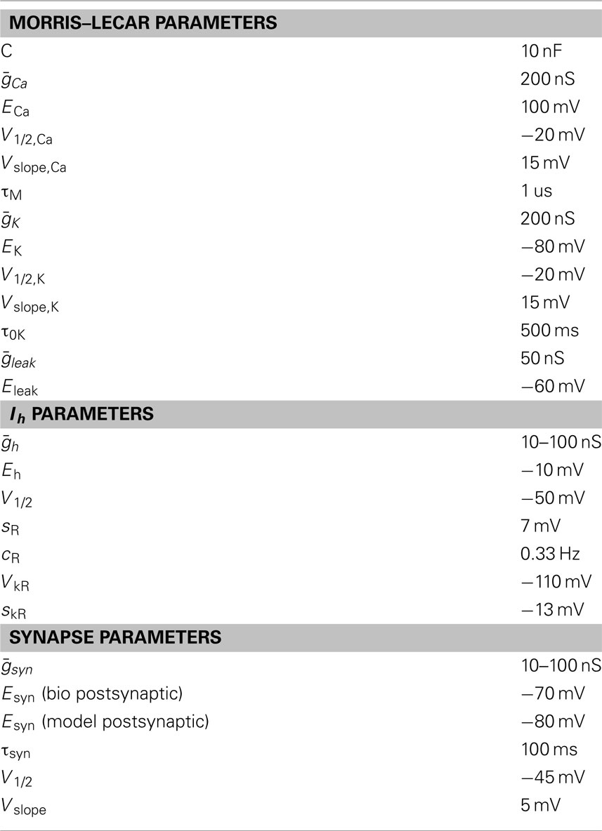
Table 1. Values of parameters for the Morris–Lecar model cell, artificial hyperpolarization-activated currents, and artificial inhibitory synapses.

The artificial I_h (Buchholtz et al., 1992; Sharp et al., 1996) was described by the equations:

$\begin{array}{l}{I}_{\text{h}}={\overline{g}}_{\text{h}}R\left(E_{\text{h}}-V\right)\\ \frac{dR}{dt}=k_{\text{R}}\left(R_{\infty }-R\right)\end{array}$

where

$\begin{array}{l}{R}_{\infty }\left(V\right)=\frac{1}{1+\exp \left[\left(V-V_{1/2}\right)/s_{\text{R}}\right]}\\ k_{\text{R}}\left(V\right)=c_{\text{R}}\left\{1+\exp \left[\left(V-V_{\text{kR}}\right)/s_{\text{kR}}\right]\right\}\end{array}$

where ${\overline{g}}_{\text{h}}$ (varied from 10 to 100 nS) was the maximal conductance of I_h; R was the instantaneous activation; R_∞ was the steady-state activation; E_h was the I_h reversal potential; V_1/2 was the half-maximum activation; s_R was the step width; c_R was the rate constant; V_kR was the half-maximum potential for the rate; and s_kR was the step width for the rate.

The artificial inhibitory graded transmission synapse from the Morris–Lecar model to the biological cell was based on Sharp et al. (1996) and was described by the following equations:

$\begin{array}{l}{I}_{\text{syn}}={\overline{g}}_{\text{syn}}\cdot S\cdot \left(E_{\text{syn}}-V_{\text{post}}\right)\\ \left(1-S_{\infty }\right){\tau }_{\text{syn}}\frac{dS}{dt}=\left(S_{\infty }-S\right)\end{array}$

where

$S_{\infty }\left(V_{\text{pre}}\right)=\left\{\begin{array}{cc}\tanh \left[\left(V_{\text{pre}}-V{}_{1/2}\right)/V_{\text{slope}}\right]& \text{if\hspace{0.17em}}{V}_{\text{pre}}>V_{1/2}\\ 0& \text{otherwise}\end{array}\right\}$

where ${\overline{g}}_{\text{syn}}.$(varied from 10 to 100 nS) was the maximal synaptic conductance; S was the instantaneous synaptic activation; S_∞ was the steady-state synaptic activation. The reversal potential of the synaptic current, E_syn, had different values in the two synapses: −80 mV when the biological neuron was postsynaptic, and −70 mV when the Morris–Lecar model was postsynaptic. V_pre and V_post are the presynaptic and postsynaptic potentials, respectively; τ_syn was the time constant for synaptic decay; V_1/2 was the synaptic half-activation voltage and V_slope was the synaptic slope voltage.

Assaying Half-Center Activity

Network activity was classified into one of four categories. If the biological cell did not fire action potentials and had no oscillation, the network was “silent.” If the biological cell had no spikes but did have a slow membrane potential oscillation, the network was “model dominated.” If the biological cell fired action potentials, the network was either “half-center” or “bio-dominated.” In half-center networks, the biological cell had slow membrane potential oscillations, and the predominant flow of synaptic current was from the bursting cell (the biological cell, then the model cell in alternation) to the non-bursting cell greater than 90% of the time.

Finding Correlations between NAPs and IPs

For each IP, we searched for subsets of NAPs that were highly correlated with it. Conversely for each NAP we searched for subsets of IPs that were highly correlated with it. Both analyses were required because the problem is inherently asymmetric: it is possible for each individual NAP to be well-explained by a linear combination of IPs, but conversely have no individual IP that is well-explained by a linear combination of NAPs. We describe the algorithm to find subsets of NAPs that are highly correlated with an IP; the converse algorithm is identical, only with the data sets swapped.

We formed matrices M_IP and M_NAP, whose rows denote identity and whose columns denote different IPs and NAPs respectively. We z-scored each matrix column to eliminate the effects of scaling and offset. For each IP (column of M_IP) we searched for a subset of NAPs (columns of M_NAP) and linear coefficients that approximated the column of M_IP. For a given subset of NAPs we formed a reduced matrix R_NAP that contained only the columns corresponding to the properties we chose, then performed linear regression to find the best linear coefficients. We assessed the quality of this fit, or “prediction error” as mean square error per degree of freedom, where the number of degrees of freedom was the number of rows (STG neurons) minus the number of columns of R_NAP (properties in the subset). We associated this prediction error with the subset of NAPs, and found the best subset of NAPs by minimizing the prediction error with greedy feature selection.

Greedy Feature Selection

The greedy algorithm is a heuristic approach to searching a large space of candidate features. It quickly selects a very good subset of features, although not necessarily the best. We initialized the greedy algorithm by creating an empty set of features, and declaring its prediction error to be infinite. We then proceeded iteratively as follows:

1. Form every subset of features that can be created by adding either one or two new properties to the current best subset.

2. Compute the prediction error of all the new subsets.

3. If any has a prediction error lower than the current best subset, select the subset with the lowest prediction error as the new best, and iterate again; otherwise stop.

At the end of iteration, the output of the greedy algorithm was the best subset of features and their prediction error.

Assigning p-values to Correlations

Given enough properties, we expect to see large correlations between some of them, even if they are merely random numbers. This is exacerbated by the greedy algorithm, because it discovers the largest correlations and ignores small ones. To determine whether the correlations in the data were large enough to be likely real, we computed the probability that equally large correlations would be found randomly in uncorrelated data.

Correlations in data are related to ordering. Independently scrambling the order of rows of M_IP and rows of M_NAP eliminates any correlations between IPs and NAPs, while preserving their distributions as well as the relationships within the IPs and within the NAPs. Performing the greedy search for correlations on these scrambled data returns the prediction errors for correlations between unrelated data. Because there are many ways to scramble the rows, we did this repeatedly (10,000 scrambled trials) and obtained an empirical estimate of the null distribution for prediction errors. The p-value of a correlation arising randomly is the proportion of prediction errors in the null distribution that is lower than the prediction error from the unscrambled data.

Correcting for Multiple Correlations

Because of the need to assign many p-values, we expected that several might yield apparently “significant” results by chance, thus p-values needed to be adjusted to compensate for this problem. We describe a method for evaluating and correcting p-values obtained from scrambled data, that is conceptually similar to the Holm–Bonferroni correction (Holm, 1979; Aickin and Gensler, 1996) for multiple comparisons. A fit to scrambled data is expected to occasionally produce outliers with very low errors, although it is not clear that these outliers would be concentrated on any particular IP or NAP. Thus to determine if our best fit is likely due to chance, we compare our best fit to the best fit for each scrambled trial, regardless of which property gave the best fit in the different scrambled trials.

Therefore we started by sorting the prediction errors from the correlation search into increasing order. Then we proceeded iteratively as with the Holm–Bonferroni technique, starting with the best fit (least prediction error). We sorted the prediction error from each scrambled trial into increasing order, generating an empirical estimate of the null distribution of the best fit. The adjusted p-value for the fit was the proportion of scrambled best fits that had lower error. If the adjusted p-value did not meet the significance criterion (p < 0.05) the fit and all higher error fits were not significant and the iteration stopped. Otherwise the fit was significant, and the corresponding property was removed from consideration in future p-values, both in the scrambled and unscrambled data. For example, if property P_3 was the best fit and was found to be significant, then P_3 would be removed from each scrambled trial regardless of whether it was the best fit for that scrambled trial. Then the iteration would continue with the next best fit. In this way (similar to Holm–Bonferroni), the best overall fit is compared to the best of N scrambled fits, the second-best is compared to N − 1, etc., until one of the fits is not significant. Furthermore, the data being removed from consideration are data that have already been shown to have correlations significantly better than chance.

Linear Classification

Linear classifiers were constructed of four binary classifiers, one for each neuronal type. Each binary classifier computed the likelihood that a set of properties belonged to a cell corresponding to the classifier’s type. The likelihood function for binary classifiers was a logistic function acting on a linear function of z-scored neuronal properties (Bishop, 1996; Taylor et al., 2006). If there are N properties, then the likelihood L was calculated as

$L\left(\vec{w}\right)=P\left(w_{\text{0}}\text{ + }{p}_{\text{1}}*w_{\text{1}}+p_{\text{2}}*w_{\text{2}}+\dots +p_N*w_N\right)\text{,}$

where p_n are the z-scored properties, w_n are the weights (w₀ is an offset), and P is the logistic function,

$P\left(x\right)=\frac{1}{1+exp\left(-x\right)}.$

The weights for all binary classifiers were trained simultaneously using the whole dataset (or a subset if we were using cross-validation). To minimize the weights, we used a “soft max” function

$S=\frac{L_{\text{correct}}}{L_{\text{DG}}+L_{\text{PD}}+L_{\text{GM}}+L_{\text{LP}}},$

where L_DG, L_PD, L_GM, and L_LP were the likelihoods computed for each cell type, and L_correct is the likelihood for the correct cell type for a given cell. When training the classifier, we maximized the sum of the log-likelihood of S over the whole dataset (or a subset if we were using cross-validation),

$\vec{w}=arg\hspace{0.17em}max\sum _{k\in \left\{\text{neurons}\right\}}log\left(S_{\text{k}}\left(\vec{w}\right)\right)$

The optimization was performed using an iterative line-search method (Bishop, 1996), initialized with Fisher’s linear discriminant (Bishop, 1996). When determining the results of the trained classifier, we determined the cell type as the one with the greatest likelihood.

To determine how well linear classification generalized, we used leave-two-out cross-validation. Thousand trials were conducted. In each trial the properties for two randomly chosen neurons were selected to be test data, and a linear classifier was trained on the remaining data. After the classifier was trained, the test data were classified. The cross-validation accuracy was the proportion of test data that were classified correctly.

Finding Clusters

We used k-medoids (Hastie et al., 2009) to categorize blindly STG neurons based on their z-scored properties. We set k = 4 and measured distance between points using L₁ (taxicab) norm. The k-medoids algorithm was initialized using the same procedure as k-means++ (Arthur and Vassilvitskii, 2007). Because the initialization is not deterministic, we used 200 trials, using the results of the trial that had the smallest average distance from each point to its medoid.

The results of the clustering allow construction of a contingency table called a “confusion matrix.” The rows of the matrix correspond to STG cell type, the columns to cluster label, and the entries are the number of cells so categorized [e.g., the gastric mill (GM), 2 entry corresponds to the number of GM cells grouped into cluster 2]. Cluster labels were assigned the cell identity that maximized the proportion of cells correctly identified (proportion correct). Mutual information (MI) was computed as in Vinh et al. (2009). Adjusted mutual information (AMI) was computed as

$\text{AMI}=\frac{\text{MI}-\overline{\text{MI}}}{{\text{MI}}_{\max }-\overline{\text{MI}}},$

where $\overline{\text{MI}}$ is the expected value of MI for a random clustering, and MI_max is the maximum possible MI. MI_max was computed as in Vinh et al. (2009). We computed $\overline{\text{MI}}$ as the mean of the distribution of MI for random clustering, generated using a bootstrap technique.

Generating the Distribution of Mutual Information via Bootstrap

We modeled the confusion matrix as being generated by binomial random numbers [e.g., if two out of 13 dorsal gastric (DG) neurons were in cluster 1, the DG,1 entry was modeled as binomial random with a maximum value of 13 and an expectation value of 2]. From a given confusion matrix, we randomly generated synthetic confusion matrices using the same binomial distributions for each entry, and computed MI from these synthetic confusion matrices. We used 10,000 synthetic confusion matrices to generate an empirical distribution of MI. Because the clustering algorithm will always place at least one cell in every cluster, any synthetic confusion matrices with a column of all zeros were discarded and regenerated. To generate the MI distribution for real data sets, we used the confusion matrix generated by the results of the k-medoids algorithm. To generate the MI distribution for clustering of random data sets, we used a confusion matrix with identical columns, and rows that summed to the number of cells in our actual data set (e.g., the sum of the DG row was equal to the number of DG cells in our data).

Computing p-values for Differences in Clustering

We did not seek to compute a rigorous probability that one set of properties is inherently superior to another with regard to clustering performance. Instead we asked if the difference in MI between two clustering results (MI_low and MI_high) can be plausibly ascribed merely to fluctuations in the number of cells in each cluster. To compute p between two clusterings, we used the bootstrap method to obtain the distribution of MI_low. We then calculated p as the proportion of synthetic MI_low that is greater than the actual MI_high. We called differences with p < 0.05 “significant.”

Source Code

Source code implementing the statistical methods that we developed is hosted permanently at http://www.bio.brandeis.edu/MarderLabCode/

Results

The STG of the crab C. borealis has 26–27 neurons, that can be reliably identified according to their projection patterns (Marder and Bucher, 2007). Each STG has two pyloric dilator (PD) neurons, one lateral pyloric (LP) neuron, four GM neurons, and one DG neuron. The data in this paper come from 55 neurons (PD n = 13; LP n = 15; GM n = 14; DG n = 13). The PD and LP neurons are part of the circuit that generates the fast (period ∼1 s) pyloric rhythm and the GM and DG neurons are part of the circuit that generates the slow (period 6–10 s) GM rhythm.

Conventional IPs were measured by injecting current steps and ramps into individual neurons to measure input resistance, spike threshold voltage, FI slope, spike frequency with 1 nA injected current, spike height, and minimum voltage with zero injected current. Figure 1A shows a recording of a DG neuron in response to a current ramp, showing the voltage at threshold and the spike height. Figure 1B shows the same cell in response to depolarizing current pulses of different amplitudes. Figure 1C shows the plot of spike frequency vs. injected current. Spike frequency with 1 nA injected current can be read directly from this plot, while the linear fit (blue line) allows determination of FI slope. Figure 2 summarizes all of the IPs that went into the analysis, with the new data points in color, and those from the prior study (Grashow et al., 2010) in gray. Note that the variance of each measure is considerable, and there is a great deal of overlap across cell types.

FIGURE 1

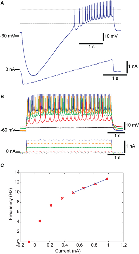
Figure 1. Traditional IPs for one DG neuron. (A,B) Membrane potential is shown in the top trace, and injected current in the bottom trace. (A) Spike threshold voltage is the voltage at the point of maximum curvature (dashed line) before the first spike in response to a ramp of injected current. (B) The FI curve was obtained by measuring spike frequency in response to depolarizing current steps. (C) FI Slope is the slope of the best-fit line to the linear region of the FI curve. For this DG neuron, the four rightmost points were used (see Materials and Methods). The spike rate in response to 1 nA of injected current is (in this case) the last data point.

FIGURE 2

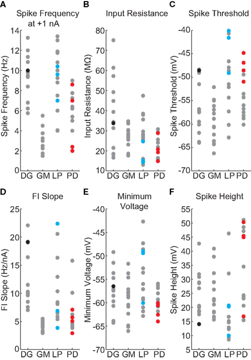
Figure 2. Values of IPs, by neuron type. New data points are in color, and those from the prior study (Grashow et al., 2010) are in gray. (A) Spike frequency with 1 nA injected current. (B) Input resistance. (C) Spike threshold voltage. (D) Frequency–current slope. (E) Minimum voltage with zero injected current. (F) Spike height.

Because of the overlap in these measures even across neurons with very different characteristic behaviors during ongoing network activity, we reasoned that a set of properties that better captured the potential dynamics of the neurons in a closed-loop dynamic network might be more useful in characterizing these neurons than the conventional, open-loop IPs shown in Figure 1.

Stomatogastric ganglion neurons are part of circuits that are rhythmically active, so we sought a measure that would place these neurons into a rhythmically active circuit under experimenter control. Therefore we used the dynamic clamp to create two-cell circuits: one cell being the neuron to be evaluated, the second a standard model neuron used in all experiments. Figure 3 shows the result of a dynamic clamp experiment in which an isolated DG neuron was coupled with reciprocal inhibition to a Morris–Lecar model neuron (Morris and Lecar, 1981; Grashow et al., 2010), and the strength of the synaptic conductances $\left({\overline{g}}_{\text{syn}}\right)$ and an imposed I_h conductance $\left({\overline{g}}_{\text{h}}\right)$ were varied. A schematic of this circuit is shown in Figure 3A. Figure 3B shows the behavior of the model neuron and the biological neuron in the uncoupled state, and Figures 3C,D show different patterns of resulting network activity. Figure 3E illustrates the case in which the model and biological neurons are firing in alternating bursts of activity, or half-center oscillations. We obtained NAPs exclusively by examining networks with half-center activity, because these were precisely the networks that exhibited rhythmic activity with the complex mix of spiking and slow membrane potential oscillations that characterizes the membrane potential trajectories that STG neurons display during ongoing pyloric and gastric mill rhythms.

FIGURE 3

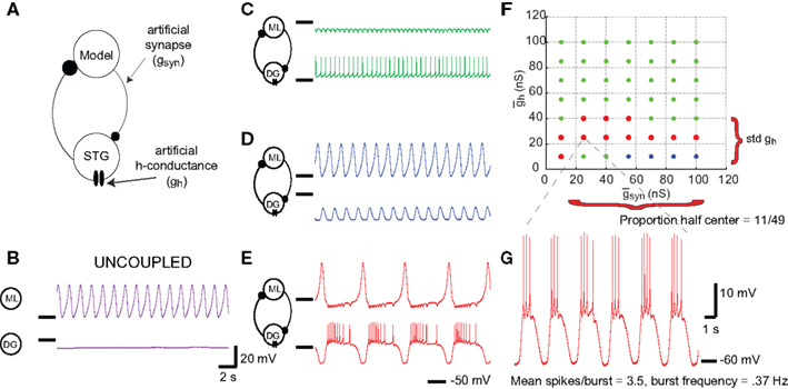
Figure 3. Network activity of the artificial circuit depends on $\left({\overline{g}}_{\text{syn}},{\overline{g}}_{\text{h}}\right)$ parameter values. (A) Schematic for two-cell synthetic circuit. A model Morris–Lecar neuron is connected to a biological STG neuron (either DG, GM, LP, or PD) via artificial mutual inhibitory synapses. Dynamic clamp simulated the synapses, as well as injecting artificial h-conductance into the STG neuron. (B) Voltage traces from uncoupled $\left({\overline{g}}_{\text{syn}}=0,{\overline{g}}_{\text{h}}=0\right)$Morris–Lecar model (top) and DG neuron (bottom). (C–E) Voltage traces from connected circuit with different $\left({\overline{g}}_{syn},{\overline{g}}_h\right)$ parameter values. Colors denote network activity classification: green traces denote networks dominated by the DG neuron, blue denotes networks dominated by the Morris–Lecar neuron, and red denotes networks exhibiting half-center oscillations. (C) ${\overline{g}}_{\text{syn}}=70,$${\overline{g}}_{\text{h}}=55.$ (D) ${\overline{g}}_{\text{syn}}=85,$${\overline{g}}_{\text{h}}=10.$ (E) ${\overline{g}}_{\text{syn}}=40,$${\overline{g}}_{\text{h}}=40.$ (F,G) NAPs are representative of a biological neuron’s overall response to all of the $\left({\overline{g}}_{syn},{\overline{g}}_h\right)$ parameter values in a map. (F) The proportion of half-center networks is trivially obtained from the map. Std ${\overline{g}}_{\text{h}}$ is the SD of ${\overline{g}}_{\text{h}}$ values among half-center networks. (G) Spikes per burst and half-center frequency are both obtained from individual networks, then averaged over all half-center networks.

Figure 3F shows a map of the network behavior as ${\overline{g}}_{\text{syn}}$ and ${\overline{g}}_{\text{h}}$ were varied. The map positions that produced half-center alternating bursts are shown in the red dots. For each of the 55 experiments, we used these maps to calculate the proportion of map positions that resulted in half-center activity. In the map shown in Figure 3F, this proportion was 11/49. For each set of parameters that gave half-center activity (map positions with alternating bursts) we calculated the half-center frequency and the number of spikes/burst in the biological neuron (Figure 3G). Because each biological neuron used had a different set of IPs, we expected that the map produced with each one would be different. The hypothesis was that features of these maps and of their half-center behavior (size, location, burst frequencies, number of spikes/burst of half-center activity) would constitute a data set that might more reliably capture the neurons’ dynamics, and consequently their cellular identity, than the conventional measures of intrinsic excitability.

Figure 4 presents the data from all of the half-centers found in the 55 experiments analyzed. In most of the maps half-center activity was found in a horizontal swath, indicating that half-center activity was more sensitive to ${\overline{g}}_h$ than to ${\overline{g}}_{syn}$. The SD of ${\overline{g}}_h$ provides a measure of the width of the horizontal swath. Figure 4A shows that although the variance of this measure for each cell type is considerable, the PDs had a larger SD than the other cell types. The proportion of half-centers in the 55 neurons is shown in Figure 4B. The mean half-center frequency was higher in the PD neuron set of networks (Figure 4C), and mean number of spikes/burst was lowest in the networks made with GM neurons (Figure 4D).

FIGURE 4

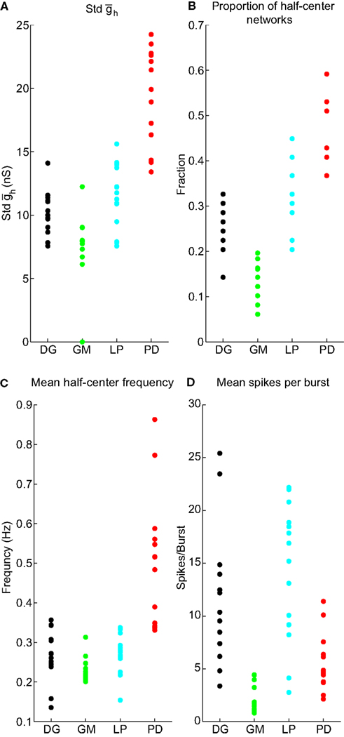
Figure 4. Values of NAPs, by neuron type. (A) Std ${\overline{g}}_{\text{h}}$. (B) Proportion of half-center networks. (C) Mean half-center frequency. (D) Mean spikes per burst.

We refer to the four measures – “SD of ${\overline{g}}_{\text{h}},$” “proportion of half-center networks,” “mean half-center frequency,” and “mean spikes per burst” – as NAPs. There are many conceivable network properties; however we restricted the analysis to a handful that were simple to measure and that we reasoned would be related to both IPs and cell identity.

Correlations between NAPs and IPs

We first asked if there is any predictive relationship between these measures of network activity and conventional IPs. For each IP, we searched for the subset of NAPs that best predicted it (see Materials and Methods). Conversely, we looked for the subset of IPs that best predicted each NAP.

To assess the significance of any correlations we repeated the predictive analysis on 10,000 shuffled trials (see Materials and Methods). In a shuffled trial, we scrambled the cell identity while preserving the distribution of individual properties. The shuffled trials provided an empirical estimate of the null distribution for prediction error; and because the null distribution was estimated from trials with multiple correlations, we were able to correct for multiple correlations and calculate adjusted p-values (see Materials and Methods).

The results of this analysis are detailed in Table 2. Figure 5 shows selected scatter-plots of several properties vs. the values predicted by their best-fit linear combination. Three of the six IPs were significantly predicted by NAPs, and all of the NAPs were significantly predicted by IPs. However, the R² values of the correlations were low, indicating weak predictive value.

TABLE 2

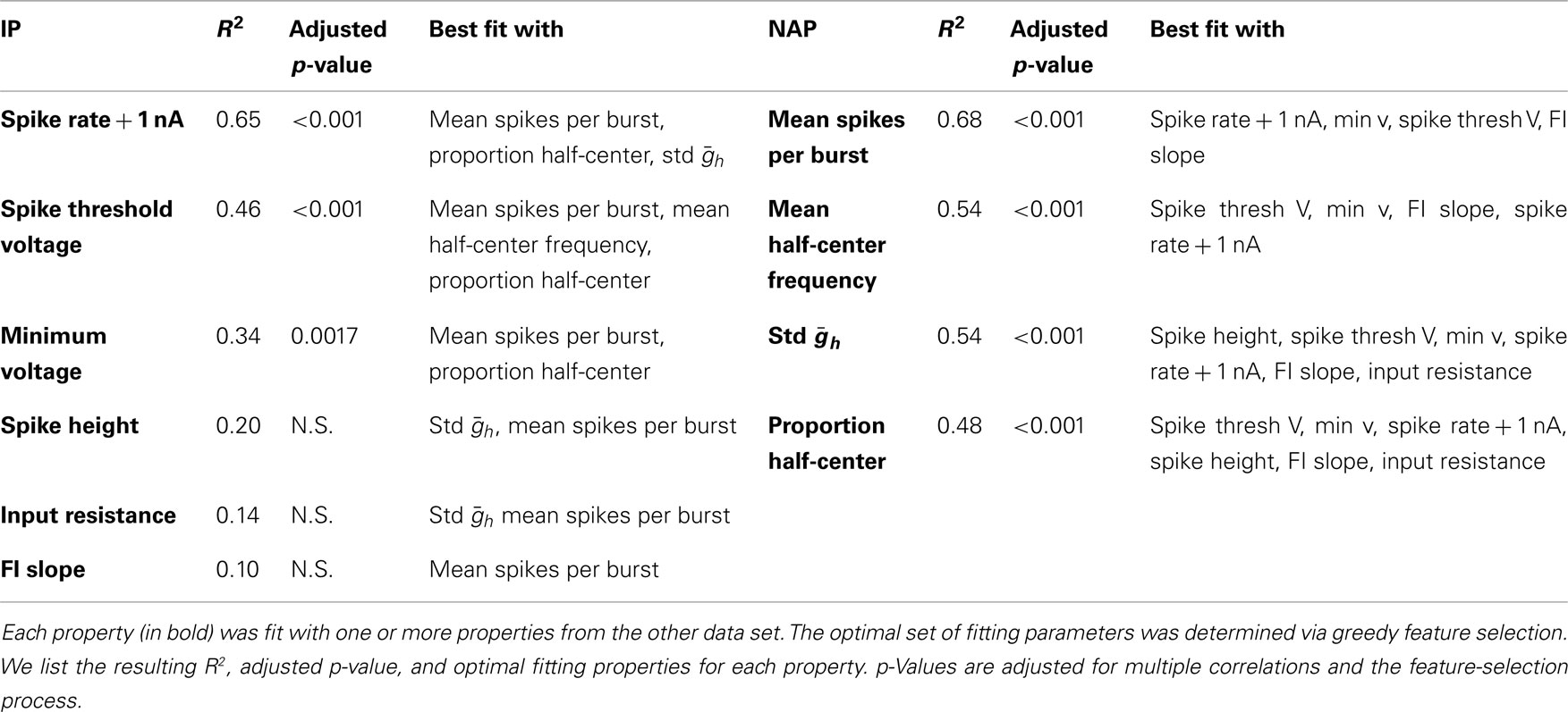
Table 2. Correlations between IPs and NAPs.

FIGURE 5

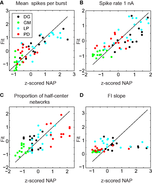
Figure 5. Sample fits of z-scored neuronal properties. Value of the property being fit (x) vs. value predicted by the best regression (y). The line y = x corresponds to a perfect fit. (A) Mean spikes per burst was best fit simultaneously to spike rate 1 nA, minimum voltage, spike threshold voltage, and FI slope (R² = 0.68, p < 0.001). (B) Spike rate 1 nA was best fit simultaneously to mean spikes per burst, proportion of half-center networks, and std ${\overline{g}}_h$ (R² = 0.65, p < 0.001). (C) Proportion of half-center networks was best fit simultaneously to spike threshold voltage, minimum voltage, spike rate 1 nA, spike height, FI slope, and input resistance (R² = 0.48, p < 0.001). (D) FI slope had no significant correlations, but was best fit with mean spikes per burst (R² = 0.10, p > 0.05).

Linear Classifier

We next asked whether we could reliably determine the identity of the four neuron types using the six measurements of IPs (Figure 2), using the four measurements of NAPs taken from the dynamic clamp networks (Figure 4) or by combining the two sets of data together. Given the large range of these measurements within a cell type and the overlap of the values across the cell types, it is clear that no single measure would reliably allow the identification of the neurons.

To identify neuron types by their properties, the different cell types must have properties that segregate into different clusters. To check if this is the case, we attempted to train a linear classifier to determine neuronal identity based on a given set of z-scored properties. The classifier was constructed of four binary linear classifiers, one for each neuronal class. Binary classifiers estimated the likelihood that a neuron’s properties corresponded to the binary classifier’s STG type. The likelihood was a number between zero and one; whichever binary classifier returned the highest likelihood “won,” and the overall classifier then determined that the properties belonged to a neuron of the corresponding type.

Conceptually, for a set of N properties, a linear classifier describes four N − 1 dimensional oriented hyperplanes (one for each binary classifier), with all the neurons of the correct type on the “plus” side of a hyperplane, and the remaining neurons on the “minus” side. In practice, the situation may be less straightforward, with all four hyperplanes being in compromise positions, allowing their pooled information to determine identity. In such a situation, placement, and orientation of hyperplanes may depend on outlier points, especially when the number of cells is small but N is large.

We trained a linear classifier for each set of properties. The classifier based on IPs identified 85% of cells correctly, the classifier based on NAPs identified 84% correctly, and the combined properties classifier identified 100% of cells correctly (Figure 6). However, these high accuracies were partially due to overfitting outlier points. When we tested the generalizability of these classifiers with leave-two-out cross-validation (see Materials and Methods), the accuracy of each classifier dropped somewhat: IPs classified 64% correctly, NAPs 68%, and the combined data 78%. Thus only by combining the two data sets can the cell types be distinguished on the basis of properties, and even then the boundary between them is complex and dependent upon the position of outlier points.

FIGURE 6

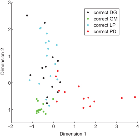
Figure 6. A linear classifier can be trained to correctly identify cell type. Hundred percentage of neurons were correctly identified when a linear classifier was trained on combined IPs and NAPs. To visualize the grouping of neurons by property, we projected the 10-dimensional space of properties down to two dimensions. Analogously to the results of Principal Component Analysis, we determined components (combinations of properties) that pointed along directions of particular interest. These directions (Dimension 1 and Dimension 2) were chosen to provide maximal spacing between the different neuronal types.

Finding Clusters

Ideally, one would like to identify neuron types blindly, not merely verify that they fall into properties of clusters. This approach would be applicable to a system where cells cannot be unambiguously identified as they can in the STG. We used the k-medoids algorithm (Hastie et al., 2009) with k = 4 to find clusters of properties. However, clusters do not directly correspond to any particular cell type (i.e., after running k-medoids, a cell is labeled “cluster 2” not “GM”). To address this issue, we computed two measures of accuracy. We assigned cluster labels to cell identity to maximize the number of cells that are correctly categorized, and computed the “proportion correct.” This number is necessarily in the interval between 1/k and 1. We also computed the MI between the cluster labels and the cell identities. By appropriately scaling the MI we computed the AMI which has a maximum value of one, and an expected value of zero for random numbers. In addition to our real data, we applied the clustering technique to a synthetic set of properties generated from Gaussian random numbers, to illustrate chance results. We used a bootstrap technique to estimate p-values for significant differences in MI between clusterings.

Both of the accuracy measures (MI/AMI and proportion correct) showed the same general trends. No set of properties was able to correctly identify all cells. When we performed k-medoids clustering on Gaussian random numbers, as expected we obtained no information (proportion correct = 0.29, MI = 0.089, AMI = −0.002). Real neuronal properties were able to obtain significant information: for IPs proportion correct = 0.60, MI = 0.36, and AMI = 0.21; for NAPs proportion correct = 0.69, MI = 0.72, and AMI = 0.49; and for both sets joined proportion correct = 0.84, MI = 0.90, and AMI = 0.62. The results of clustering on the combined properties are depicted in Figure 7A. All sets of STG properties achieved results significantly better than random numbers, with p < 0.001. The differences between sets of properties were also significant (NAPs vs. IPs p = 0.01, combined properties vs. IPs p < 0.001, combined properties vs. NAPs p = 0.03). The quantification of accuracy is summarized in Figure 7B. Together these results show that NAPs encode more information about cell identity than traditional IPs, but both sets contain distinct information (Figure 7C).

FIGURE 7

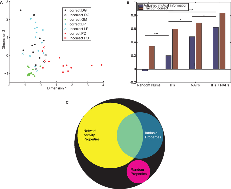
Figure 7. IPs and NAPs partially encode neuronal identity. (A) k-Medoids clustering was applied to the combined IPs and NAPs of STG neurons. Filled circles denote correctly classified neurons, Xs denote errors. The 10-dimensional space is projected down to two dimensions that best separate the different neuronal types. (B) Adjusted mutual information (blue) and proportion correct (red) by property type. p-Values between clustering results are computed by the technique described in Section “Materials and Methods.” *p < 0.05, ***p < 0.001. (C) A Venn diagram depicting the information encoded by the two sets of properties, assuming improved encoding of the combined sets is due to non-overlapping mutual information. The area of the black circle depicts perfect encoding of cell identity, while the magenta circle describes the mutual information expected from a set of randomly generated properties.

Discussion

Establishing reasonable and reliable methods for classifying and characterizing neurons has been a far thornier practical problem than might have been predicted from first principles. While there are large and uniquely identifiable neurons in small invertebrate nervous systems and in the spinal cords of fish and frogs, in most regions of the vertebrate central nervous system and in many brain areas in invertebrates, cell identification cannot be achieved by size or location of the neurons alone. The electrophysiological firing patterns of many neurons change (Dickinson et al., 1990; Weimann et al., 1991), either as a consequence of neuromodulation, development, or disease. Transmitter phenotype (Borodinsky et al., 2004) and transcription factor expression (William et al., 2003; Wienecke et al., 2010) are often developmentally or activity regulated, complicating the use of a single chemical marker to identify neurons, although chemical markers may be sufficient at times (Zagoraiou et al., 2009). Neuronal projection patterns to distant targets such as muscles or other brain regions often provide unambiguous identification, but when multiple cell types are entangled in local circuits, even projection patterns may not be sufficient. These issues are further confounded by the large variance measured in a variety of properties of individual neurons (Getting, 1981; Hume and Getting, 1982; Swensen and Bean, 2005; Schulz et al., 2006, 2007; Goaillard et al., 2009; Tobin et al., 2009; Grashow et al., 2010). This raises the question of whether combining multiple measures can serve to better cluster or identify neurons, and if so, what kinds of assays are potentially more useful than conventional measures of intrinsic excitability.

In this study we used six conventional measures of neuronal IPs and four measures of how neurons behaved in an artificial network to determine whether any or all of these measures could correctly cluster and identify neurons whose identity was already known. This exercise highlighted a number of difficulties that, to a greater or lesser degree, will potentially plague investigators wishing to use electrophysiological measures to identify neurons. It is clear from the variance in each of the IPs across individual neurons of the same class and from the overlap of these values across cell types, that no single measure would reliably serve to identify the neurons (Figure 2; Grashow et al., 2010). Therefore, our goal was to determine whether the combined set of electrophysiological measures would reliably allow us to cluster the neurons into groups that mapped correctly with their identity.

One might naively think that increasing the number of electrophysiological measures performed for each neuron would increase the likelihood of proper identification. This might appear to be especially the case if each measure probes a different essential feature of the cell’s performance. For that reason, we chose to embed each neuron in an artificial network that we reasoned would test its dynamic behavior differently than the conventional measures of excitability. Nonetheless, increasing the number of measures made for each neuron tested comes with a statistical cost, as each additional increases the likelihood of finding spurious correlations. Because it is necessary to correct for this before assigning statistical significance, adding measures that even partially sample the same biophysical attributes to a neuron may be more counterproductive than helpful. For some cell types a different set of measured IPs or NAPs might be more useful than those studied here. Nonetheless, our point is simply to say that “more is not necessarily better.” To this end, in choosing the NAPs that we included, we used our biological intuition to select four that appeared to be relatively functionally independent of each other, and we discarded many other potential network measures that might have added relatively little to the analysis and added a substantial multiple comparison statistical burden. Obviously, these problems are more acute with relatively modest-sized data sets, such as that analyzed here, and become less acute with data sets with n’s in the several thousand (at which point it is also possible to use additional methods).

Because STG neurons can be recorded from intracellularly for many hours it was experimentally feasible for us to ask whether these NAPs would be useful in neuron characterization. We were surprised that the networks did not provide more information than they did, and we do not expect or recommend that an investigator working in systems where recordings cannot be maintained for many hours attempt the same process, although other closed-loop measures that are less time-consuming could be devised.

We assessed significance of correlations with a custom bootstrapping method that combines shuffled trials and the Holm–Bonferroni correction for multiple comparisons. It is commonly assumed that correlations do not need to be corrected because they are only indicative of interesting relationships, not a rigorous test in themselves. However, the process of finding correlations may be too effective – if it can find seemingly strong correlations in random data, then there may be confusion between correlations that are indicative of real relationships, and those that are most likely spurious.

Data-mining commonly produces large spurious correlations. When we simply applied a Pearson correlation test, every correlation was “significant” and there were several p-values less than 10⁻¹⁰. Using shuffled trials properly accounts for the power of data-mining and dramatically increased the magnitude of the p-values (many were still highly significant). Building Holm–Bonferroni into the procedure allowed further correction for investigating many properties.

Although these two methods (comparing to shuffled trials, and adjusting p-values with the Holm–Bonferroni method) are commonly used separately, we are not aware of them being used together as done here. However, we believe it is necessary to combine them because we had no a priori hypothesis about which correlations were likely to be most significant. After searching a data set for correlations we find several with varying strengths, and want to know which correlations are weak enough that they could plausibly be drawn from the distribution of expected spurious correlations. To do this it was necessary to keep track of all the correlations for each shuffled trial, and therefore integrate the multiple comparisons correction into the shuffled trial structure.

The results of our correlation analysis appear to differ from Grashow et al. (2010) which analyzed much of the same data. However it should be borne in mind that the two analyses ask different questions. Grashow et al. (2010) asked, “What are the pairwise relationships between these different properties?”, while here we asked “How well can we reconstruct one set of properties from the other?” Both are potentially interesting questions, and have their strengths and weaknesses.

Grashow et al. (2010) tested all possible pairwise correlations (48 total) between larger property sets. Because of this, their correction for multiple comparisons was quite large. We searched for the best linear reconstruction for each property (10 total), thus incurring a smaller penalty for multiple comparisons. However the approach here may not find all the correlations that are of potential interest. For instance, if an NAP is highly correlated with two IPs, and those two IPs are highly correlated with each other, then this approach is unlikely to discover that the NAP is correlated with both IPs. More likely it would only discover one of them. This is because adding the second IP will decrease the degrees of freedom without substantially improving the fit, leading the combination to be heavily discounted by the feature-selection algorithm. Thus some of the differences between the two studies result from asking different questions.

However, some differences between the studies were due to improvements in methodology. As is often done, Grashow et al. (2010) computed adjusted p-values by using the Pearson correlation coefficient test for normally distributed data, then applying the Holm–Bonferroni correction for multiple comparisons. These data exhibit deviations from normality (e.g., Figure 2F, where LP exhibits substantial skew, and PD appears to be bimodal) and thus the Pearson correlation test is not fully appropriate. Furthermore the Holm–Bonferroni correction may be overly conservative because it does not account for potential relationships between the different quantities whose correlation is being tested. Here, basing the significance test on scrambled trials, we avoided making assumptions about the distribution of the data. By incorporating the adjustment for multiple correlations into the scrambled trials, we directly computed the approximate null distribution for the nth-best correlation. This enabled us to compute a p-value that is conservative enough to account for multiple correlations without being unnecessarily over-conservative.

In general, the methods we used – searching for correlations and clustering – decrease in effectiveness as the dimensionality they must work in (the number of properties) increases. Increasing dimensionality increases the probability of finding correlations between random numbers, making corrections for multiple correlations more severe and therefore decreasing the ability to detect real correlations. Clustering algorithms suffer from a host of problems referred to collectively as “the curse of dimensionality” (Bishop, 1996; Beyer et al., 1999; Hinneburg et al., 2000; Houle et al., 2010), which cause them to find the “wrong” clusters. It is especially difficult if extraneous dimensions are added, because algorithms naturally tend to break up clusters at essentially meaningless gaps in the extraneous dimensions. We decreased the number of properties we considered to avoid this problem as much as possible.

In this analysis the information pertaining to cell identity can be thought of as a Venn diagram (Figure 7C), with IPs containing some information, NAPs containing more information, and some overlap between the two sets. It is possible that because we used six measures of IPs, thus a higher dimension than the NAPs, they are merely falling afoul of the curse of dimensionality and thus unfairly penalized when compared to the four NAPs. However, when the two sets are grouped together the resulting set of properties has still higher dimensionality and outperforms either one separately, suggesting that the Venn diagram is appropriately representing the data. Looking at the raw MI if we naively assume that non-overlapping information combines additively, we see that the NAPs contain roughly twice as much information as the IPs, and that roughly half the information in the IPs is in the overlapping region of the Venn diagram (Figure 7C). Thus the NAPs do capture the neuronal dynamics of each cell type better than the conventional measures of IPs, although we cannot perfectly identify neurons only by their properties. The success of NAPs suggests that closed-loop dynamic current perturbations yield greater information about cell identity than static perturbations. However, the properties extracted from this perturbation must be chosen carefully, because the size of the data sets will never be large enough to search through the essentially infinite space of all possible properties.

We used k-medoids, one of the simplest clustering algorithms (Andreopoulos et al., 2009), but not always the best. The k-medoids algorithm is nearly the same as the k-means algorithm, however clusters are represented by one of the members of the cluster (called the “medoid,” and chosen to minimize distance to other members of the cluster) rather than the mean of members of the cluster. k-Medoids is more robust to outliers than k-means (Andreopoulos et al., 2009; Hastie et al., 2009) and is applicable in situations when computing mean objects is impossible or undesirable. k-Medoids is slower than k-means with very large data sets [selecting the medoid is O(N²) while computing the mean is O(N)]. However, as is common for electrophysiology, the data set studied here is small and we expect plentiful outliers due to the variability in neurons and noise inherent in measuring neuronal properties. In principle, more sophisticated density-based (Sander et al., 1998), nearest-neighbor-based (Ertöz et al., 2003; Bohm et al., 2004; Pei et al., 2009; Kriegel et al., 2011), or correlation-based (Kriegel et al., 2008) methods are capable of determining the number of clusters, recognizing extraneous dimensions, and finding clusters with complex shapes. When deciding on the methods we would use for this paper, we conducted pilot tests for a variety of clustering algorithms on synthetic data sets of a size comparable to our IPs and NAPs. In these pilot tests, we found that the more sophisticated clustering algorithms were less successful at identifying cluster membership (i.e., neuronal identity) correctly. With small data sets, there were inevitably extraneous large density fluctuations or extraneous correlations, therefore for this study, k-medoids was superior by virtue of being simpler, but this would certainly change with a larger data set. These results suggest that with a large number of neurons and a small number of highly relevant properties, identifying cells via clustering is likely to be fruitful.

In this analysis we implemented corrections for multiple comparisons and methods to determine the statistical significance of the resulting correlations. In many studies reporting correlations, corrections for multiple correlations were not made. Obviously, if the correlations are robust, they will persist after the appropriate corrections are made. Nonetheless, it is likely that some reported correlations in the literature would not have survived a more rigorous statistical analysis. Of course, it is essential to remember that a weak correlation may point to a fundamental biological insight, while a strong correlation may not always help illuminate an underlying biological process.

Conflict of Interest Statement

The authors declare that the research was conducted in the absence of any commercial or financial relationships that could be construed as a potential conflict of interest.

Acknowledgments

We thank Dr. Adam Taylor for useful discussions. This work was supported by MH467842, T32 NS07292, and NS058110 from the National Institutes of Health.

References

Aickin, M., and Gensler, H. (1996). Adjusting for multiple testing when reporting research results: the Bonferroni vs Holm methods. Am. J. Public Health 86, 726–728.

Pubmed Abstract | Pubmed Full Text | CrossRef Full Text

Andreopoulos, B., An, A., Wang, X., and Schroeder, M. (2009). A roadmap of clustering algorithms: finding a match for a biomedical application. Brief. Bioinformatics 10, 297–314.

Pubmed Abstract | Pubmed Full Text | CrossRef Full Text

Arthur, D., and Vassilvitskii, S. (2007). “k-Means++: the advantages of careful seeding,” in Proceedings of the Eighteenth Annual ACM-SIAM Symposium on Discrete Algorithms. (New Orleans, LA: Society for Industrial and Applied Mathematics), 1027–1035.

Beyer, K., Goldstein, J., Ramakrishnan, R., and Shaft, U. (1999). When is “nearest neighbor” meaningful?” in Database Theory – ICDT’99, eds C. Beeri and P. Buneman (Berlin: Springer), 217–235.

Bishop, C. M. (1996). Neural Networks for Pattern Recognition. Oxford: Oxford University Press.

Bohm, C., Railing, K., Kriegel, H. P., and Kroger, P. (2004). “Density connected clustering with local subspace preferences,” in ICDM ‘04. Fourth IEEE International Conference on Data Mining, 2004, Piscataway, 27–34.

Borodinsky, L. N., Root, C. M., Cronin, J. A., Sann, S. B., Gu, X., and Spitzer, N. C. (2004). Activity-dependent homeostatic specification of transmitter expression in embryonic neurons. Nature 429, 523–530.

Pubmed Abstract | Pubmed Full Text | CrossRef Full Text

Buchholtz, F., Golowasch, J., Epstein, I. R., and Marder, E. (1992). Mathematical model of an identified stomatogastric ganglion neuron. J. Neurophysiol. 67, 332–340.

Pubmed Abstract | Pubmed Full Text

Calabrese, R. L., Norris, B. J., Wenning, A., and Wright, T. M. (2011). Coping with variability in small neuronal networks. Integr. Comp. Biol. 51, 845–855.

Pubmed Abstract | Pubmed Full Text | CrossRef Full Text

Dickinson, P. S., Mecsas, C., and Marder, E. (1990). Neuropeptide fusion of two motor pattern generator circuits. Nature 344, 155–158.

Pubmed Abstract | Pubmed Full Text | CrossRef Full Text

Dorval, A. D., Christini, D. J., and White, J. A. (2001). Real-time linux dynamic clamp: a fast and flexible way to construct virtual ion channels in living cells. Ann. Biomed. Eng. 29, 897–907.

Pubmed Abstract | Pubmed Full Text | CrossRef Full Text

Ertöz, L., Steinbach, M., and Kumar, V. (2003). “Finding clusters of different sizes, shapes, and densities in noisy, high dimensional data,” in Proceedings of the Third SIAM International Conference on Data Mining, eds D. Barbará and C. Kamath (San Francisco: Society for Industrial and Applied Mathematics), 12.

Getting, P. A. (1981). Mechanisms of pattern generation underlying swimming in Tritonia. I. Neuronal network formed by monosynaptic connections. J. Neurophysiol. 46, 65–79.

Pubmed Abstract | Pubmed Full Text

Getting, P. A. (1989). Emerging principles governing the operation of neural networks. Annu. Rev. Neurosci. 12, 185–204.

Pubmed Abstract | Pubmed Full Text | CrossRef Full Text

Getting, P. A., and Dekin, M. S. (1985). Mechanisms of pattern generation underlying swimming in TRITONIA. IV. Gating of central pattern generator. J. Neurophysiol. 53, 466–480.

Pubmed Abstract | Pubmed Full Text

Getting, P. A., Lennard, P. R., and Hume, R. I. (1980). Central pattern generator mediating swimming in tritonia. I. Identification and synaptic interactions. J. Neurophysiol. 44, 151–164.

Pubmed Abstract | Pubmed Full Text

Goaillard, J. M., Taylor, A. L., Schulz, D. J., and Marder, E. (2009). Functional consequences of animal-to-animal variation in circuit parameters. Nat. Neurosci. 12, 1424–1430.

Pubmed Abstract | Pubmed Full Text | CrossRef Full Text

Grashow, R., Brookings, T., and Marder, E. (2010). Compensation for variable intrinsic neuronal excitability by circuit-synaptic interactions. J. Neurosci. 30, 9145–9156.

Pubmed Abstract | Pubmed Full Text

Hastie, T., Tibshirani, R., and Friedman, J. (2009). The Elements of Statistical Learning: Data Mining, Inference, and Prediction. New York: Springer Verlag, 515–520.

Hinneburg, A., Aggarwal, C. C., and Keim, D. A. (2000). “What is the nearest neighbor in high dimensional spaces?” in Proceedings of the 26th International Conference on Very Large Data Bases (San Francisco: Morgan Kaufmann Publishers Inc.) 671675, 506–515.

Holm, S. (1979). A simple sequentially rejective multiple test procedure. Scand. J. Stat. 6, 65–70.

Houle, M., Kriegel, H.-P., Kröger, P., Schubert, E., and Zimek, A. (2010). “Can shared-neighbor distances defeat the curse of dimensionality?” in Scientific and Statistical Database Management, eds M. Gertz and B. Ludäscher (Berlin: Springer), 482–500.

Hume, R. I., and Getting, P. A. (1982). Motor organization of tritonia swimming. II. Synaptic drive to flexion neurons from premotor interneurons. J. Neurophysiol. 47, 75–90.

Pubmed Abstract | Pubmed Full Text

Hume, R. I., Getting, P. A., and Del Beccaro, M. A. (1982). Motor organization of tritonia swimming. I. Quantitative analysis of swim behavior and flexion neuron firing patterns. J. Neurophysiol. 47, 60–74.

Pubmed Abstract | Pubmed Full Text

Jonas, P., Bischofberger, J., Fricker, D., and Miles, R. (2004). Interneuron diversity series: fast in, fast out – temporal and spatial signal processing in hippocampal interneurons. Trends Neurosci. 27, 30–40.

Pubmed Abstract | Pubmed Full Text | CrossRef Full Text

Katz, P. S. (1996). Neurons, networks, and motor behavior. Neuron 16, 245–253.

Pubmed Abstract | Pubmed Full Text | CrossRef Full Text

Kriegel, H.-P., Kröger, P., Sander, J., and Zimek, A. (2011). Density-based clustering. Wiley Interdiscip. Rev. Data Min. Knowl. Discov. 1, 231–240.

CrossRef Full Text

Kriegel, H.-P., Kröger, P., Schubert, E., and Zimek, A. (2008). “A general framework for increasing the robustness of PCA-based correlation clustering algorithms,” in Scientific and Statistical Database Management, eds B. Ludäscher and N. Mamoulis (Berlin: Springer), 418–435.

Kristan, W. B. Jr., Calabrese, R. L., and Friesen, W. O. (2005). Neuronal control of leech behavior. Prog. Neurobiol. 76, 279–327.

Pubmed Abstract | Pubmed Full Text | CrossRef Full Text

Marder, E., and Bucher, D. (2001). Central pattern generators and the control of rhythmic movements. Curr. Biol. 11, R986–R996.

Pubmed Abstract | Pubmed Full Text | CrossRef Full Text

Marder, E., and Bucher, D. (2007). Understanding circuit dynamics using the stomatogastric nervous system of lobsters and crabs. Annu. Rev. Physiol. 69, 291–316.

Pubmed Abstract | Pubmed Full Text | CrossRef Full Text

Marder, E., and Calabrese, R. L. (1996). Principles of rhythmic motor pattern generation. Physiol. Rev. 76, 687–717.

Pubmed Abstract | Pubmed Full Text

Meyrand, P., Simmers, J., and Moulins, M. (1991). Construction of a pattern-generating circuit with neurons of different networks. Nature 351, 60–63.

Pubmed Abstract | Pubmed Full Text | CrossRef Full Text

Miller, J. P., and Selverston, A. I. (1982a). Mechanisms underlying pattern generation in lobster stomatogastric ganglion as determined by selective inactivation of identified neurons. II. Oscillatory properties of pyloric neurons. J. Neurophysiol. 48, 1378–1391.

Miller, J. P., and Selverston, A. I. (1982b). Mechanisms underlying pattern generation in lobster stomatogastric ganglion as determined by selective inactivation of identified neurons. IV. Network properties of pyloric system. J. Neurophysiol. 48, 1416–1432.

Miller, M. N., Okaty, B. W., and Nelson, S. B. (2008). Region-specific spike-frequency acceleration in layer 5 pyramidal neurons mediated by Kv1 subunits. J. Neurosci. 28, 13716–13726.

Pubmed Abstract | Pubmed Full Text | CrossRef Full Text

Morris, C., and Lecar, H. (1981). Voltage oscillations in the barnacle giant muscle fiber. Biophys. J. 35, 193–213.

Pubmed Abstract | Pubmed Full Text | CrossRef Full Text

Mulloney, B., and Selverston, A. I. (1974a). Organization of the stomatogastric ganglion in the spiny lobster. I. Neurons driving the lateral teeth. J. Comp. Physiol. 91, 1–32.

CrossRef Full Text

Mulloney, B., and Selverston, A. I. (1974b). Organization of the stomatogastric ganglion in the spiny lobster. III. Coordination of the two subsets of the gastric system. J. Comp. Physiol. 91, 53–78.

CrossRef Full Text

Okaty, B. W., Sugino, K., and Nelson, S. B. (2011a). Cell type-specific transcriptomics in the brain. J. Neurosci. 31, 6939–6943.

CrossRef Full Text

Okaty, B. W., Sugino, K., and Nelson, S. B. (2011b). A quantitative comparison of cell-type-specific microarray gene expression profiling methods in the mouse brain. PLoS ONE 6, e16493. doi:10.1371/journal.pone.0016493

CrossRef Full Text

Pearson, K. G., Reye, D. N., Parsons, D. W., and Bicker, G. (1985). Flight-initiating interneurons in the locust. J. Neurophysiol. 53, 910–925.

Pubmed Abstract | Pubmed Full Text

Pei, T., Zhu, A. X., Zhou, C., Li, B., and Qin, C. (2009). Detecting feature from spatial point processes using collective nearest neighbor. Comput. Environ. Urban Syst. 33, 435–447.

CrossRef Full Text

Perrins, R., and Weiss, K. R. (1996). A cerebral central pattern generator in Aplysia and its connections with buccal feeding circuitry. J. Neurosci. 16, 7030–7045.

Pubmed Abstract | Pubmed Full Text

Sander, J., Ester, M., Kriegel, H.-P., and Xu, X. (1998). Density-based clustering in spatial databases: the algorithm GDBSCAN and its applications. Data Min. Knowl. Discov. 2, 169–194.

CrossRef Full Text

Sasaki, K., Due, M. R., Jing, J., and Weiss, K. R. (2007). Feeding CPG in Aplysia directly controls two distinct outputs of a compartmentalized interneuron that functions as a CPG element. J. Neurophysiol. 98, 3796–3801.

Pubmed Abstract | Pubmed Full Text | CrossRef Full Text

Schmidt, J., Fischer, H., and Buschges, A. (2001). Pattern generation for walking and searching movements of a stick insect leg. II. Control of motoneuronal activity. J. Neurophysiol. 85, 354–361.

Pubmed Abstract | Pubmed Full Text

Schulz, D. J., Goaillard, J. M., and Marder, E. (2006). Variable channel expression in identified single and electrically coupled neurons in different animals. Nat. Neurosci. 9, 356–362.

Pubmed Abstract | Pubmed Full Text | CrossRef Full Text

Schulz, D. J., Goaillard, J. M., and Marder, E. E. (2007). Quantitative expression profiling of identified neurons reveals cell-specific constraints on highly variable levels of gene expression. Proc. Natl. Acad. Sci. U.S.A. 104, 13187–13191.

Pubmed Abstract | Pubmed Full Text | CrossRef Full Text

Selverston, A. I., and Miller, J. P. (1980). Mechanisms underlying pattern generation in the lobster stomatogastric ganglion as determined by selective inactivation of identified neurons. I. Pyloric neurons. J. Neurophysiol. 44, 1102–1121.

Pubmed Abstract | Pubmed Full Text

Selverston, A. I., Russell, D. F., Miller, J. P., and King, D. G. (1976). The stomatogastric nervous system: structure and function of a small neural network. Prog. Neurobiol. 7, 215–290.

Pubmed Abstract | Pubmed Full Text | CrossRef Full Text

Sharp, A. A., Skinner, F. K., and Marder, E. (1996). Mechanisms of oscillation in dynamic clamp constructed two-cell half-center circuits. J. Neurophysiol. 76, 867–883.

Pubmed Abstract | Pubmed Full Text

Sugino, K., Hempel, C. M., Miller, M. N., Hattox, A. M., Shapiro, P., Wu, C., Huang, Z. J., and Nelson, S. B. (2006). Molecular taxonomy of major neuronal classes in the adult mouse forebrain. Nat. Neurosci. 9, 99–107.

Pubmed Abstract | Pubmed Full Text | CrossRef Full Text

Swensen, A. M., and Bean, B. P. (2005). Robustness of burst firing in dissociated Purkinje neurons with acute or long-term reductions in sodium conductance. J. Neurosci. 25, 3509–3520.

Pubmed Abstract | Pubmed Full Text | CrossRef Full Text

Taylor, A. L., Hickey, T. J., Prinz, A. A., and Marder, E. (2006). Structure and visualization of high-dimensional conductance spaces. J. Neurophysiol. 96, 891–905.

Pubmed Abstract | Pubmed Full Text | CrossRef Full Text

Tobin, A. E., Cruz-Bermudez, N. D., Marder, E., and Schulz, D. J. (2009). Correlations in ion channel mRNA in rhythmically active neurons. PLoS ONE 4, e6742. doi:10.1371/journal.pone.0006742

CrossRef Full Text

Toledo-Rodriguez, M., and Markram, H. (2007). Single-cell RT-PCR, a technique to decipher the electrical, anatomical, and genetic determinants of neuronal diversity. Methods Mol. Biol. 403, 123–139.

Pubmed Abstract | Pubmed Full Text | CrossRef Full Text

Vinh, N. X., Epps, J., and Bailey, J. (2009). “Information theoretic measures for clusterings comparison: is a correction for chance necessary?” in Proceedings of the 26th Annual International Conference on Machine Learning (Montreal, QC: ACM), 1073–1080.

Weimann, J. M., and Marder, E. (1994). Switching neurons are integral members of multiple oscillatory networks. Curr. Biol. 4, 896–902.

Pubmed Abstract | Pubmed Full Text | CrossRef Full Text

Weimann, J. M., Meyrand, P., and Marder, E. (1991). Neurons that form multiple pattern generators: identification and multiple activity patterns of gastric/pyloric neurons in the crab stomatogastric system. J. Neurophysiol. 65, 111–122.

Pubmed Abstract | Pubmed Full Text

Wienecke, J., Westerdahl, A. C., Hultborn, H., Kiehn, O., and Ryge, J. (2010). Global gene expression analysis of rodent motor neurons following spinal cord injury associates molecular mechanisms with development of postinjury spasticity. J. Neurophysiol. 103, 761–778.

Pubmed Abstract | Pubmed Full Text | CrossRef Full Text

William, C. M., Tanabe, Y., and Jessell, T. M. (2003). Regulation of motor neuron subtype identity by repressor activity of Mnx class homeodomain proteins. Development 130, 1523–1536.

Pubmed Abstract | Pubmed Full Text | CrossRef Full Text

Zagoraiou, L., Akay, T., Martin, J. F., Brownstone, R. M., Jessell, T. M., and Miles, G. B. (2009). A cluster of cholinergic premotor interneurons modulates mouse locomotor activity. Neuron 64, 645–662.

Pubmed Abstract | Pubmed Full Text | CrossRef Full Text