Assisted closed-loop optimization of SSVEP-BCI efficiency

Introduction

The use of closed-loop interaction with biological nervous systems for observation and control purposes goes back to the beginnings of electrophysiology in the 1940s when the voltage clamp technique was developed (Marmont, 1949; Cole, 1955). Later on, the dynamic clamp technology to implement artificial membrane or synaptic conductances (Robinson and Kawai, 1993; Sharp et al., 1993) has produced many examples of successful closed-loop interactions with neural systems at the cellular and circuit levels (for reviews see Prinz et al., 2004; Goaillard and Marder, 2006; Destexhe and Bal, 2009; Economo et al., 2010).

We recently proposed a generalization of the dynamic clamp concept in electrophysiology and animal ethology to design closed-loop interactions with biological nervous systems beyond electrical stimulation and recording. In particular, we investigated in our previous work goal-driven real-time closed-loop interactions with drug microinjectors, mechanical stimulation devices and video event driven stimulators (Muniz et al., 2008, 2011; Chamorro et al., 2009, 2012). These examples illustrate that modern activity-dependent stimulation protocols can reveal dynamics otherwise hidden under traditional stimulation techniques, provide control of regular and pathological states, induce learning processes, bridge between distinct levels of analysis and lead to a further automation of experiments. In this paper, we propose the same assisted closed-loop approach described in our previous work to optimize the efficiency of steady state visually evoked potentials (SSVEP) based brain-computer interfaces (BCI) which might have a large impact for applied uses, such as computer control and biomedical or prosthetic uses, but also as novel paradigms for basic research. Generally, the innovative assistance consists in the delivery of online information with regard to the control over the given BCI goal both to the human subject and to the system, together with the online adaptation of BCI stimuli properties.

BCIs use measures of brain activity, typically real-time human EEG recordings, usually in order to interact with devices such as virtual keyboards, etc. (for recent reviews see e.g., Birbaumer, 2006; Van Gerven et al., 2009; Nicolas-Alonso and Gomez-Gil, 2012). Among the most successful BCIs are those which rely on SSVEPs, a type of event related potentials (ERPs) generated by the nervous system in response to repetitive visual stimulation (flicker) by linear superposition of transient visually evoked potentials (VEPs) (Capilla et al., 2011) up to 90 Hz (Herrmann, 2001): apart from smaller responses in higher harmonic frequencies, the brain mainly generates electrical activity at just the same fundamental frequency as its visual system is exposed to the visual flicker frequency. SSVEPs are frequently used in basic and applied research because of their relatively large magnitudes which lead to superior signal-to-noise ratios (SNRs) and make them relatively stable against artifacts as compared to other ERPs (Vialatte et al., 2010).

SSVEP-BCIs make use of the physiological property that SSVEP magnitudes can be modulated by visual-spatial selective attention (e.g., Morgan et al., 1996). Thus, SSVEP based BCIs employ multiple visual stimuli (e.g., LEDs or regions on a screen) flickering at different frequencies. Apart from these intraindividual state changes due to attention, SSVEP magnitudes further depend both on extrinsic variables as the spatial and temporal frequencies of the stimulus, and on other intrinsic intra- and interindividual dimensions of the subjects themselves (Ding et al., 2006; Lopez-Gordo et al., 2011). The optimal spatial frequency of a structured stimulus is related to individual traits such as visual acuity or age (Vialatte et al., 2010). There is also a significant difference in the magnitude of SSVEPs between flicker stimulation of the center (fovea centralis) vs. the periphery of the visual field. Environmental conditions (e.g., screen brightness and frequency, distance to the screen, etc.) also influence the performance of the BCI. Although determined by multiple factors, SSVEP magnitudes are modulated by the subjects' states of attention. Hence, online monitoring of SSVEP magnitudes elicited by arrays of multiple flickering light sources allows BCI systems to detect to which flicker source the subject is attending to at a given moment. Taken altogether, these aspects call for automated mechanisms to optimize parameters of the stimuli and of the BCI control, aiming toward flexible adaptiveness to specific individual and contextual situations of SSVEP-BCI use.

Commonly, SSVEP-BCIs use only one prefixed set of flicker frequencies, but nonetheless there are studies employing two different prefixed sets (e.g., Volosyak et al., 2009, 2011) which lead to remarkably different results. Those findings imply that BCI efficiency may crucially depend on flicker frequency selection. Following this idea, we created an assisted closed-loop adaptive algorithm to search for the best frequencies for each subject and for each particular time point/situation of use. The adaptive and informative nature of this novel online approach aims to improve the BCI efficiency as compared to traditional paradigms (see Figure 1). Firstly, this optimization process is realized by performing a real-time closed-loop search for the best set of frequencies to achieve the given BCI goal. The number of stimuli and their effectiveness with regard to the BCI goal modulate this real-time search strategy. The closed-loop search is evaluated in real-time by a continuous measurement of the actual BCI efficiency (see section “Efficiency Measures”), which is used as an online criterion to select the BCI control parameters. Secondly, the SSVEP online recording is processed, on the one hand, to an online auditory feedback to inform the subject and, on the other, is used to inform the system to select the best flicker frequencies. This shared information constitutes the assisted part of the closed-loop. The proposed protocol aims to address the problems which arise from different hardware configurations, subjects' intra- and inter-individual variabilities, e.g., in neuropsychological dimensions of executive functioning (see e.g., Funahashi, 2001) etc., and other sources of variability in experimental settings and intrinsic dimensions.

FIGURE 1

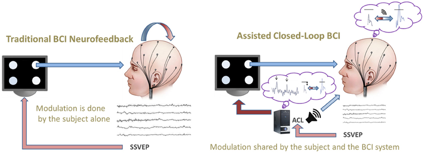
Figure 1. Comparison of a traditional BCI neurofeedback (left) vs. the novel assisted closed-loop paradigm (right) which informs both the subject (about his/her brain activity in relation to the BCI goal) and the system (about the specificities of the given subject). In our example, the assisted closed-loop provides online information (i) to the system about the most effective flicker frequencies and (ii) to the subject about the actual distance to the pre-defined threshold by continuous auditory feedback (loudspeaker symbol, right).

The paper is organized as follows: in section “Materials and Methods” the new assisted closed-loop system is described; in section “Results” analyses and correlates efficiency as compared with traditional BCI paradigms are presented; finally, in “Discussion” section we discuss about the generalization and applicability of the proposed novel protocol.

Materials and Methods

Participants

A convenience non-probability sample of N = 18 healthy subjects from our department was used applying the exclusion criteria self-reported chronic medication/substance intake and neurological diseases as e.g., epilepsy. Our sample consisted of 6 females and 12 males with age Mdn = 26.00 years (25th percentile = 23.00, 75th = 35.75), range = 18–59. Subjects had a normal or corrected-to-normal vision and were right-handed. Permission of the ethics committee of Autonomous University of Madrid was obtained; all subjects participated voluntarily in the sense of an informed consent without receiving any incentives. Participants were informed that they could leave the experiments at any time without giving any explication.

SSVEP BCI System

Stimulation device

We constructed a stimulation panel with four white color LEDs (manufacturer Seoul Semiconductor, white lamp LED LW500AM, ∅ 5 mm, viewing angle 100°), using a 100 Ω series resistor to the digital +5V output of the acquisition board (see below) which results in a luminous intensity output I_V ≈ 700 mcd for each LED.

On a black background panel, each LED was mounted into a reflector with ∅40 mm diffuser cap carrying an outstanding non-transparent cylindrical black screen of 45 mm length; the spatial organization is illustrated in Figure 2. Below each white flicker light source we placed a green color standard signaling LED to instruct the subject where to look during the BCI task. The distance of the LED stimulation panel to the subject was kept ~60 cm, resulting in a visual angle of ~3.8° for every light source.

FIGURE 2

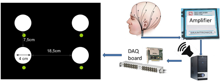
Figure 2. Diagram of the BCI flicker stimulation setup (left) and the signal acquisition/stimulation system. The flickering frequency was controlled by a software driving the digital output of a National Instruments data acquisition (DAQ) board (model NI-PCI-6251) directly connected to the white colored LEDs, generating 0/+5V off vs. on signals according to the desired flicker frequency. We verified the intended flicker frequency for each light source independently by a photodiode connected to a digital oscilloscope. Luminous intensity output is I_V ≈ 700 mcd for each white LED. Smaller green color standard signaling LEDs were placed below to instruct subjects where to look during the BCI task.

BCI task

The BCI task consisted in subjects trying to follow a prefixed sequence of 16 steps by focusing their vision onto a specific flickering white light source out of the four possible ones at each step, as continuously indicated by the smaller green signaling LEDs below. This sequence was identical for all subjects. A brief beep sound confirmed the indicated flickering light source as correctly detected.

Stimulation

We compared the BCI efficiency under three conditions of flicker frequency selection: (i) by the assisted closed-loop (ACL) protocol, (ii) by a standard protocol with stimulation frequencies prefixed at 27, 28, 29, and 30 Hz (because 1 Hz distances are commonly employed in SSVEP-BCIs e.g., Herrmann, 2001; Diez et al., 2011; Volosyak et al., 2011), and (iii) by a protocol which used a selection of top frequencies for each subject (see section “ACL Algorithm”). In order to compensate for possible presentation order effects, the order of (i), (ii), y (iii) was permutated over the subjects.

Figure 3 shows the timeline of the experiment. The first phase of the experiment consisted in the measurement of the individual EEG baseline and the frequency scanning phase to select a set of flicker stimulation frequencies for each subject (the number of frequencies in this set is specific for each participant—see below). The second phase is the BCI phase with its three conditions (i), (ii), and (iii) mentioned above.

FIGURE 3

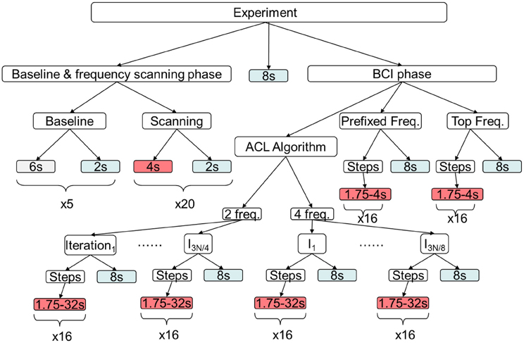
Figure 3. Timeline of the experiment. In the first phase individual EEG baseline activity is measured and in the following frequency scanning phase those frequencies electing largest SSVEP magnitudes are selected for each subject individually, while those below a predefined threshold are excluded (Top Freq.). Later, these values are used in the BCI phase. Under the prefixed frequency condition, always the same frequency set of 27, 28, 29, and 30 Hz is used for stimulation. Red boxes indicate stimulation, blue resting periods and gray baseline recording; in each box durations are reported.

Signal Acquisition and Preprocessing

The signal acquisition and preprocessing steps are summarized in Figure 4. The EEG signal was recorded at 1024 Hz with eight sintered Ag/AgCl electrodes mounted into a “Aegis Array” stretch lycra cap (Sands Research Inc., Texas/USA) using a “BRAINBOX^® EEG-1166” 64 channel EEG amplifier (Braintronics B.V, Almere/Netherlands) with in-house software written in C. Vertical and horizontal EOG was recorded bipolarly by an in-house battery driven analog amplifier following a circuitry of Usakli and Gurkan (2010) with sintered Ag/AgCl electrodes fixed by adhesive rings above/below the left eye vs. at left/right epicanthus connected to a data acquisition board (NI-PCI-6251, National Instruments) at 1024 Hz. The eight standard 10–20 positions were FPz, F3, Fz, F4, Cz, Pz, POz, and Oz (Jasper, 1958). For online SSVEP detection as BCI input only POz and Oz were used, while for later offline studies the signals from all eight mentioned electrodes were analyzed. The EEG reference electrode was placed at nose tip, EOG ground electrode at glabella and impedances were kept <10 kΩ.

FIGURE 4

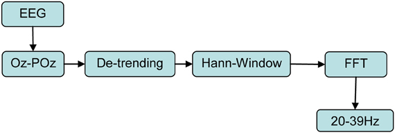
Figure 4. Signal chain of acquisition and online preprocessing. Input signals are the time domain EEG signals at electrodes Oz and POz sampled at 1024 Hz which finally result in normalized SSVEP spectral power densities S_f for each of the 20 stimulation frequencies f using as transformation to frequency domain the Fast Fourier Transform (FFT).

To improve SSVEP detection, we used the online computed difference signal between Oz and POz as bipolar montage as the only input signal to our BCI system. This reduces both EOG/EMG artifacts and EEG activity not related to the visual cortex because this montage implements a simple and computationally inexpensive spatial high pass filter (see Figure 5). Thus, the SNR for the SSVEP detection is increased as compared to unipolar montages (Diez et al., 2010). In a time window of 2 s, this difference signal was then linearly detrended, treated by a Hann-window and then converted into frequency domain by Fast Fourier Transform (FFT) with a window length of 2048 sample points. The chosen Hann-window function has a quite narrow main lobe, which determines a good frequency resolution, and reasonable side lobe suppression (Harris, 1978). Those FFT coefficients meeting the exact flicker frequencies were used, one single coefficient for each flicker frequency. Thus, 20 real numbers were obtained and squared to represent the power spectral densities (PSDs) in the flicker range 20–39 Hz (see Figure 4). This procedure was developed following Diez et al. (2011). The described analysis was continuously repeated as sliding windows with a displacement of 250 ms, resulting in 87.5% overlapping. With all four LEDs emitting steady light, magnitudes of baseline EEG activities B_f were measured over 30 s at each future flicker stimulation frequency, determined as M_PSD by the described procedure (5 sets of 6s with 2 s resting periods in between, see Figure 3 Baseline). Subjects were instructed to use only the resting periods in-between for eye blinks/relaxation and otherwise maintain their eyes quietly open, trying to avoid jaw and tongue movements to reduce EOG/EMG artifacts.

FIGURE 5

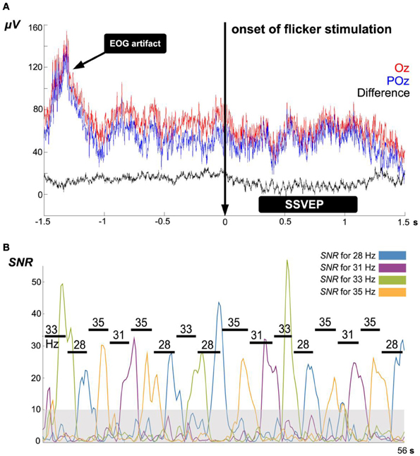
Figure 5. (A) Example of EEG time domain signals during 3 s before and after 21 Hz flicker stimulation at electrodes Oz (red) and POz (blue). Using their difference signal (black) as BCI input, in the sense of a bipolar montage, remarkably reduces common DC offsets, EOG/EMG artifacts and EEG contributions other than due to the visual cortex: the difference signal offers a simple spatial high-pass filter. (B) Example of signal-to-noise ratios S_f during a single iteration of the algorithm ACL using four different flicker frequencies. The gray shadowed area represents the noise floor with dimensionless value 10; this level was defined as SSVEP detection threshold for all subjects. Horizontal lines indicate the detection duration of each target frequency at each step.

For the frequency scanning phase of the experiment an identical measurement procedure was used, but with time windows for flicker stimulation of 4 s in each frequency f of the 20–39 Hz range resulting in magnitudes of SSVEPs as response, R_f. Each stimulation epoch is followed by a 2 s resting period. In the BCI phase of the experiment, the same procedure is used for the selected stimulation frequencies in a single measurement window of 2 s.

SSVEP PSD magnitudes were normalized to EEG baseline activity in a given frequency f as dimensionless signal-to-noise ratios:

$\begin{array}{cc}{S}_f=R_f/B_f& (1)\end{array}$

In order to minimize fatigue, we tried to keep the baseline and frequency scanning phase as short as possible, 40 s in total for the baseline and 160 s for frequency scanning.

ACL Algorithm

Selection of the top frequencies for each subject

A closed-loop approach is used to select the set of the four top stimulation frequencies by compatibility for each subject and in the given experimental context. As a first step, the specified range is scanned which results in a-priori score for each of them. Stimulation frequencies are defined as valid if their S_f exceeds a prefixed threshold (set to 10) any time during the ongoing flicker stimulation. For N valid frequencies, the frequency corresponding to the largest S_f gets an initial score of s₁(0) = N, the second to best s₂(0) = N − 1, etc. The frequency corresponding to the lowest S_f gets a score of s_N(0) = 1. Finally, the four best scores define the selection of the four top stimulation frequencies.

First closed-loop in the ACL-algorithm: iterative selection of the most compatible frequencies

The previous procedure provides initial scores for each frequency s₁(0), s₂(0),…, s_N(0) which depend on subjects' intra- and interindividual state and trait dimensions and on the extrinsic conditions in which the BCI is used. The selection of the four stimulation frequencies is then further optimized in an iterative approach attending to their compatibility. Thus, as the next step, we calculate the following compatibility measure between all possible pairs of frequencies x and y taking into account a measure of their distance and their scores:

$\begin{array}{cc}{c}_{xy}(t)=\alpha ·\left(s_x(t)+s_y(t)\right)+\beta ·d_{xy}& (2)\end{array}$

Here t represents the iteration number. We assigned the following weights to the distance and the scores: α = 1.5 and β = 1, respectively, where d_xy is a measure of the distance between the frequencies which we define below. The values for α and β were set empirically based on several trials. Because four frequencies are used simultaneously in our specific BCI implementation, the most compatible four frequencies have to be selected out of N valid frequencies, determined by the protocol described above: the first step is to identify pairs of frequencies with optimal compatibility (“2 freq.” search in the ACL branch in Figure 2). This search consists of 3N/4 iterations (see below), each of them divided into 16 steps with a resting period at its end. The ACL departs from the scores calculated in the scanning procedure s₁(0), s₂(0),…, s_N(0): they are modified in the successive iterations to search for the best compatibility.

In each iteration, the subject has to follow a sequence of flicker light sources by focusing upon them, as continuously indicated by the location of the green light. The flicker frequencies are chosen by selecting max_xy(c_xy) at the end of the iteration. To update the scores, we take into account both the success rate and the time as:

$\begin{array}{cc}{s}_x(t)=s_x(t-1)·(\delta ·\text{SR\hspace{0.17em}}-\gamma ·T)& (3)\end{array}$

where SR is the success rate (correct SSVEP detections over 16, the number of possible detections) and δ and γ are parameters of the ACL algorithm which were set to δ = 1.2 and γ = 0.02. T is the duration of the detection in seconds. The values for δ and γ were chosen based upon the range of SR and T and several simulations.

In this first part of the algorithm, the distance between two specific frequencies f_x and f_y for Equation (2) is calculated as:

$\begin{array}{cc}{d}_{xy}=\left|f_x-f_y\right|& (4)\end{array}$

Each c_xy(t) is updated by the new scores after each iteration. Once this procedure has run p = ⌊3N/4⌋ times, the highest c_xy(p) is selected and a new set is created with the union of both frequencies. Now, the next highest c_x′y′(p) disjoint from the previous set is chosen and a new set is constructed. This is repeated ⌊N/2⌋ times because this is the total number of possible disjoint pairs. It is ensured that each set is disjoint from all others. p = ⌊3N/4⌋ is chosen to test ⌊3N/2⌋ frequencies, so that the best frequencies are tested more than once. It is important to note that the duration of the frequency tests has to be restricted.

Afterwards, the second part of the algorithm is performed, the selection of four frequencies. The same procedure as in the first part is employed, but instead of single frequencies, sets of two frequencies are used. The values of s_x′(p + 1) of each set are adjusted according to the values c_xy(p), where x′ = x ∪ y. In this way, the set with the highest value gets s_1′(p + 1) = ⌊N/2⌋, the second best s_2′(p + 1) = ⌊N/2⌋ − 1 and so on. The last one gets s_⌊N/2⌋′ (p + 1) = 1. From this point of the algorithm on, these sets are indivisible.

Using the same procedure performed with two frequencies, the process is repeated with four of them. The compatibility and the score actualization rules are still the same. The only difference is the distance measure for Equation (2) calculated as:

$\begin{array}{cc}{d}_{xy}=\frac{{\displaystyle {\sum }_{i=1}^{2k}{\displaystyle {\sum }_{j=1}^{2k}\left|f_i-f_j\right|}}}{2k·(2k-1)}& (5)\end{array}$

where k is the number of frequencies of each set (in this case 2), and f_i and f_j are the individual frequencies taken from the union of the sets x and y. Note that here x and y refer to sets of two frequencies while in Equation (4) x and y referred to individual frequencies. This distance expresses the arithmetic mean of all possible pairs in the set resulting from the union of the initial sets x and y. Note that for k = 1, this distance measure is exactly the same distance (Equation 4) as used in the first part of the algorithm. In this second part ⌊3N/8⌋ iterations are performed, which is N/2 (the number of disjoint sets) times 3/4 (see above).

Second closed-loop in the ACL-algorithm: online auditory feedback of SSVEP magnitudes

In order to offer additional dynamic information to the subject related to his/her brain activity beyond the SSVEP detection confirmation cue, we provide a continuous online auditory feedback during the trials which represents the distance between the actual state and the pre-defined goal. The feedback signal consists of a 20 possible sinusoids with a range between 100 and 575 Hz which are updated every 0.25 s. The represented distance measure is defined as the difference between the EEG-SSVEP signal to noise ratio for the target frequency (S^target_f) and the threshold. Once S^target_f has reached this threshold level, the auditory feedback is muted. Previously, subjects are instructed that their goal is to raise the pitch of the sinusoids as high as possible, and that after possible success their further goal would be trying to keep the sounds muted for 1.75 s; after this silence, the program automatically proceeds to the trial's next step. This kind of continuous auditory feedback aims to help subjects to learn to gain control in their particular way over SSVEP magnitudes by attracting their attentional resources to these voluntary attempts to increase self-regulation of their resonating brain states.

Concluding, there are two assisted closed loops in our system: the first one operates over the stimulation frequency set with the aim to directly improve the ITRs of each subject. This closed-loop informs the system about subject and environment specificities. The second one informs the subject about his/her brain activity in relation to the use of the interface and helps him/her to do so faster and more accurately. This closed loop works several times for each step of a trial.

SSVEP Detection

In order to reduce the experiment's complexity in terms of a reductionistic paradigm, we choose a simple SSVEP detection strategy in our study. During the top and prefixed frequency stimulation, the S^target_f value is calculated every 0.25 s. If this value exceeds the threshold for 1.75 consecutive seconds, then this SSVEP is defined as “detected.” The threshold value was set to 10 which reflects the observed noise flow (see Figure 5). To avoid longer waiting periods when the subject is unable to exceed the threshold, a time limit of 4 s is used, after which that step is considered as fault.

During the ACL, to favor SSVEP detection in case that the subject exceeds the threshold and more time than the 1.75 s is needed to be classified as “detected,” there is a small modification in this protocol to allow adaptive time extensions. When S^target_f exceeds the threshold in a given 0.25 s time step, the time limit is increased for another 0.25 s.

Efficiency Measures

After each iteration of the algorithm, both the success rate and time needed are saved. For the prefixed and top frequencies, standard Information Transfer Rate (ITR) is calculated:

$\begin{array}{cc}\begin{array}{l}\text{ITR}(SR,t)=({\text{log}}_2(N)+SR·{\text{log}}_2(SR)+(1-SR)·\\ {\text{log}}_2((1-SR)/(N-1)))·Norm/t\end{array}& (6)\end{array}$

where N is the number of targets (N = 4 in our case). The value SR represents the success rate and t is the time taken in minutes. Norm is a normalization value set to 960 (60 s times 16 steps in each iteration). Note that if SR ≤ 1/N, then ITR(SR, t) = 0.

In contrast to the conditions prefixed and top, ITR is measured several times during the ACL. Thus, for further a-posteriori analyses these ITR distributions have to be represented by descriptive statistics: for condition ACL therefore M and Mdn of success rates and needed times are used to calculate ITR_Mean and ITR_Median, completed by maximum ITR (ITR_Max).

Convergence Measure

For a-posteriori analyses, a convergence measure for the algorithm in terms of the stimulus frequency exploration was defined: the duration of the 2 freq. search of the algorithm is divided into two parts. For each part, the numbers of explored frequencies are determined and divided by the maximal number of possible frequencies which could be explored (twice the number of iterations). The decrease comparing this measure in the second part vs. in the first part is a sign for how much the frequency exploration is converging. As can be seen in Table 1, the number of iterations varies over the subjects. The convergence measure is not reported for the first part because in our sample all subjects had the same maximal value 1, i.e., all possible frequencies were explored. We will use this measure to discuss how the ACL algorithm seems to adapt to subjects' interindividual differences.

TABLE 1

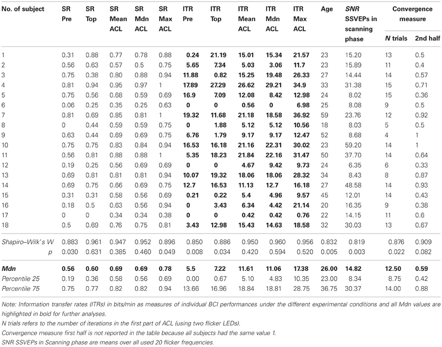
Table 1. Data of the N = 18 subjects under the three experimental conditions.

Study Design

A three conditions (ACL, top, prefixed) balanced within-subjects design with three times full permutation of presentation order (ABC, ACB, BAC, BCA, CAB, CBA) and with random assignment of subjects, resulting in N = 18 was employed.

Baseline Resting State EEG Measures as Possible Interindividual Correlates of ITR Performances

Aiming to investigate possible correlations between baseline resting state EEG measures and the variables of the experiment, the 30 s baseline EEG (see Figure 3) at all eight electrodes reported above were manually cleaned from artifacts with the result of M = 20.02 s, SD = 5.54 artifact free epochs. Under MATLAB 7.11.0.584 win64, EEG signals were preprocessed in a first step by linear detrending followed by a 8th order Butterworth 1.5–70 Hz band pass filter and finally by a 8th order Butterworth 45–55 Hz notch filter against 50 Hz power line electromagnetic interferences. Then, preprocessed EEG signals were converted into frequency domain by a sliding windows FFT transform of 2 s window length (2048 sample points) with 3.906 ms displacement (4 sample points, which correspond to a 256 Hz sample frequency in the resulting frequency domain signals), after linear detrending and treatment by a Hann-window function. Obtained FFT coefficients were squared to obtain the power spectrum and then normalized by dividing by 2048 sample points. In order to obtain absolute PSDs for the defined EEG frequencies bands of interest, corresponding coefficients were summed: thetaLow (3.5–6.5 Hz), thetaHigh (6.5–7.5 Hz); alphaLow (7.5–9 Hz), alphaHigh (9–12.5 Hz); betaLow (12.5–18 Hz), betaMid (18–24 Hz), betaHigh (18–30 Hz); totalSpectrum (0.5–70 Hz). In a first step, those absolute frequency domain PSDs signals were normalized dividing every sample point by the corresponding one of totalSpectrum which resulted in dimensionless ratios. These ratios indicate for every 256 time points per second the relative energy contribution of the frequency band of interest to the EEG total energy at this particular moment. In a last step, in order to represent EEG baseline resting state activities in the analyzed artifact free epochs by one single value for every frequency band, means of these normalized signals were computed over all corresponding time points. Thus, finally we obtained the desired baseline resting state EEG measures as relative mean PSDs for further correlational analyses, single values for every frequency band over all subjects.

Another measure of interindividual EEG variability is the resting state individual alpha frequency (IAF), because it has been found to be remarkably stable within subjects, but relatively variable between subjects (Kondacs and Szabó, 1999). In order to determine IAF in our experiment, coefficients of PSDs corresponding to the frequency band 8–13 Hz at Oz were normalized by totalSpectrum PSDs and averaged over all sliding windows in the artifact free baseline resting state epochs. In this averaged and normalized power spectrum the alpha frequency with the highest PSD was manually measured and defined as IAF (peak frequency method).

Statistical Analyses

All statistical analyses were computed using SPSS 17.0 and STATISTICA 6.0. Previously, Shapiro–Wilk tests were calculated to check each of the three conditions for normal distribution in the underlying populations. If one or more conditions showed significant departures from normality, non-parametric tests were preferred for further analyses: a Friedman test was performed as an omnibus test to investigate whether the central tendencies of one or more conditions differed significantly from the rest. In case of such a significant result, post hoc pairwise comparisons were performed in order to find out what conditions exactly differed significantly from each other, based upon comparison of mean rank differences using as significance criteria the critical rank differences proposed by the more progressive approach of Conover (1980) vs. the more conservative of Schaich and Hamerle (1984).

In order to quantify the effect sizes of those post hoc pairwise comparisons which resulted in significant differences, we used the probability of superiority of dependent scores, PS_dep, recommended by Grissom and Kim (2012) and developed in Grissom (1994). It expresses the probability that in a randomly sampled matched pair the value from the condition containing the higher scores is indeed larger than that from the one containing lower scores. PS_dep is calculated by dividing the number of positive differences between the condition containing the higher scores minus the condition containing the lower scores by the total number of matched pairs. For classifying PS_dep into small, middle and large effect sizes based upon the standards of Cohen (1988), the cut-off values reported by Grissom (1994) are used: small 0.56, medium 0.64, and large 0.71. The same author offers a table to directly convert PS into equivalent Cohen's Δ. Thus, as effect size measures both PS_dep and Cohen's Δ are reported with standards small Δ = 0.20, medium Δ = 0.50 and large Δ = 0.80 (Cohen, 1988).

In order to check whether significant differences over all six possible permutations of the presentation order might be found, a mixed-design repeated measures ANOVA was computed with stimulation condition as repeated within-subjects factor with three levels (i) ACL algorithm represented as ITR_Median, (ii) prefixed and (iii) top and presentation order as between-subjects factor with the six possible permutations as levels (ABC, ACB, BAC etc.). Previously, Levene's tests were performed in order to check for homogeneities of error variance. Moreover, the assumption of sphericity of the covariance matrix was verified previously by a Mauchly's sphericity test in order to assure that the F ratios match an F distribution. If there was a significant departure from sphericity, Greenhouse-Geisser estimates were used to correct degrees of freedom which results in fractions instead of usual integers. Although data may not follow a normal distribution, ANOVA has been demonstrated to be relatively robust against moderate deviations from normality (see e.g., Khan and Rayner, 2003). Univariate analyses were used to examine whether there is a significant between-subjects main effect of presentation order and further if there is a significant interaction effect between presentation order × stimulation condition. Analyses were repeated representing condition (i) ACL algorithm also as ITR_Mean vs. ITR_Max.

For the investigation of linear correlational relationships, Spearman's rank order correlation coefficient Rho was additionally used apart from the common Pearson product-moment correlation coefficient r due to its relative robustness firstly against outliers, but also against other than linear, but still monotonic relationships and against departures from normality or homoscedasticity. Whenever relevant influence of outliers was suspected, Spearman's rank correlation coefficient Rho was preferred.

A-priori statistical test power analyses with the program G*Power 3 (Faul et al., 2007) show that Pearson correlation significance tests in the employed sample size of N = 18 and with standard significance level α = 0.05 have test powers (1 − β) ≥ 0.80 as recommend by Cohen (1988), when they have effect sizes in the underlying population ρ ≥ 0.60, as compared to H₀: ρ = 0.00. For ρ = 0.50 test power is (1−β) ≥ 0.60, for ρ = 0.40 (1−β) = 0.40 and for ρ = 0.30 (1−β) ≈ 0.20. Thus, although the employed sample size N = 18 is relatively small, hypothesis testing of Pearson correlations with full recommended strictness is definitely possible at the level of assumed large effect sizes.

Results

Table 1 reports the data for all N = 18 subjects under the three experimental conditions, representing (i) ACL algorithm as ITR_Mean, ITR_Median and ITR_Max. Inferential statistical hypotheses testing that (i) outperformed the other two flicker stimulation conditions is reported below.

Figure 6 shows the SSVEP frequency-response curves in our experiments. For all subjects, the 20 flicker frequencies in the scanning phase were presented in the same order: 23, 37, 30, 31, 36, 22, 29, 33, 39, 24, 35, 21, 25, 27, 32, 34, 28, 20, 26, and 38 Hz. Sequential randomness of this order is confirmed with Z = −0.230 and p_exact = 0.828 (Wald–Wolfowitz runs test after Mdn split dichotomization). Our findings that in the 20–39 Hz range, lower flicker frequencies over all subjects (Figure 6A) evoke higher SSVEP magnitudes are in line with other studies which reported a global maximum SSVEP amplitude around 10 Hz with additional local maxima around 20, 40, and 80 Hz (Regan, 1989; Herrmann, 2001; Bayram et al., 2011). In our sample, we found that SSVEP frequency-response curves differed remarkably between subjects (Figure 6B) probably due to trait and state variabilities which justifies that they are determined in our experiment in the scanning phase for every subject individually.

FIGURE 6

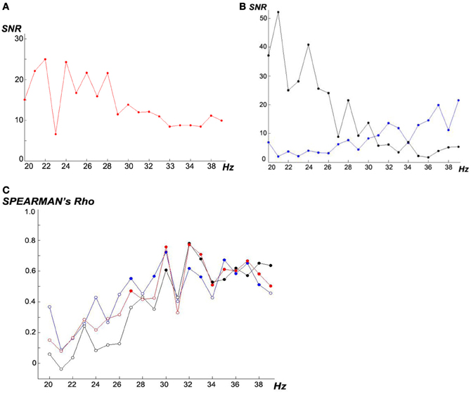
Figure 6. (A and B) SSVEP-SNR frequency-response curves. (A) Mdns over all N = 18 subjects, (B) example of two subjects with opposed frequency-response curves (black # subject 16, blue #9). (C) Frequency-dependent interindividual association between SSVEP-SNR magnitudes and ITR performances under the three experimental conditions, computed as Spearman's rank order correlations: (i) ACL algorithm (red), (ii) top (blue) and (iii) prefixed (black), filled circles represent significant p < 0.05.

Analyzing Figure 6C, higher frequencies ≥30 Hz lead to higher correlations; no relevant differences can be seen comparing the three experimental conditions. Interestingly, following e.g., Zschocke and Hansen (2012), 30 Hz is the upper boundary of beta activity observable in scalp EEGs by conventional amplifiers.

Significant and Large Improvement of SSVEP-BCI Efficiency by the Novel ACL Algorithm

Analyzing the differences in the central tendencies between the three experimental conditions (i) ACL algorithm (ii) prefixed (iii) top we represented condition (i) based upon three different descriptive statistics, (a) ITR_Mean, (b) ITR_Median, (d) ITR_Max (see section “Materials and Methods” and Table 1). Applying non-parametric inferential statistics we found a very significant and very large superiority of condition (i) ACL algorithm over the other two (ii) and (iii) which is independent of its three types of representation (a), (b), and (c), while there is no significant difference between (ii) and (iii). The used statistical methods and measures for the following results are found in section “Statistical Analyses.”

(a) A Friedman omnibus test comparing the ITRs between the three experimental conditions (i) ACL algorithm represented as ITR_Mean, (ii) prefixed and (iii) top shows a significant overall difference with χ²(2) = 10.116, p = 0.006.

Post-hoc pairwise comparisons based upon critical mean rank differences 0.82 (Schaich and Hamerle, 1984) vs. 0.58 (Conover, 1980) indicate that ITRs are significantly higher in (i) ACL algorithm as compared to (ii) prefixed (mean rank difference = 1.03, very large effect size PS_dep = 0.83, Δ = 1.37) and also as compared to (iii) top (mean rank difference = 0.64, large effect size PS_dep = 0.72, Δ = 0.83). Comparison of (ii) prefixed with (iii) top results in a non-significant difference (mean rank difference = 0.39).

(b) A Friedman omnibus test comparing the ITRs between the three experimental conditions (i) ACL algorithm represented as ITR_Median, (ii) prefixed and (iii) top shows a significant overall difference with χ²(2) = 9.262, p = 0.01.

Post-hoc pairwise comparisons based upon critical mean rank differences 0.82 (Schaich and Hamerle, 1984) vs. 0.57 (Conover, 1980) indicate that ITRs are significantly higher in (i) ACL algorithm as compared to (ii) prefixed (mean rank difference = 0.94, very large effect size PS_dep = 0.81, Δ = 1.25) and also as compared to (iii) top (mean rank difference = 0.64, very large effect size PS_dep = 0.76, Δ = 1.21) applying the less conservative criterion of (Conover, 1980). Comparison of (ii) prefixed with (iii) top results in a non-significant difference (mean rank difference = 0.31).

(c) A Friedman omnibus test comparing the ITRs between the three experimental conditions (i) ACL algorithm represented as ITR_Max, (ii) prefixed and (iii) top shows a significant overall difference with χ²(2) = 22.986, p = 0.00001.

Post-hoc pairwise comparisons based upon critical mean rank differences 0.82 (Schaich and Hamerle, 1984) vs. 0.41 (Conover, 1980) indicate that ITRs are significantly higher in (i) ACL algorithm as compared to (ii) prefixed (mean rank difference = 1.47, extremely large effect size PS_dep = 0.94, Δ = 2.25) and also as compared to (iii) top (mean rank difference = 1.19, extremely large effect size PS_dep = 0.94, Δ = 2.25). Comparison of (ii) prefixed with (iii) top results in a non-significant difference (mean rank difference = 0.28).

The ACL Algorithm Seems to Adapt to Subjects' Interindividual Differences

N_Trials in condition (i) ACL algorithm using two flicker LEDs (see Table 1) is deterministically given by 3/4 of the total number of the SSVEP-SNR responses under the 20 flicker frequencies in the scanning phase of the experiment which had exceeded the defined threshold value of 10 (suitable frequencies), see ACL Algorithm of section “Materials and Methods.” Thus, in order to make the investigation of possible interindividual associations between the SSVEP-SNR magnitudes with the convergence measure second half (see section “Materials and Methods”) relatively independent from N_Trials, all subjects with N_Trials < 25th percentile (8.75 ≈ 9) were excluded, # subject 6, 8, 9, 12, 13, and 16. The resulting rest of N = 12 subjects showed a relatively small variability with range of N_Trials between 11 and 15. The measure SSVEP-SNR mean magnitudes in the scanning phase of the experiment (a) over all flicker frequencies from 20 to 39 Hz was split into two measures, one for (b) lower frequencies from 20 to 29 Hz and the other for (c) higher frequencies from 30 to 39 Hz. In this subsample, convergence measure second half shows large and highly significant correlations with (a) of r = 0.839, p = 0.001, with (b) of r = 0.843, p = 0.001 and with (c) of r = 0.763, p = 0.004. Checking these relationships against the remaining variability of N_Trials and age as controlled third variables in partial correlation analyses, indeed no changes are observed; those found relationships can be considered as linearly independent from N_Trials and age. Hence, these findings show that the convergence of the ACL algorithm highly depends on the subjects' trait ability to generate higher SSVEP-SNR magnitudes, with no relevant differences observed between lower vs. higher flicker frequencies: focusing on a subsample with a more or less constant number of suitable frequencies, the ACL algorithm explored the more distinct frequencies in those subjects who displayed the larger SSVEP-SNR magnitudes in the scanning phase of the experiment.

In conclusion, these findings imply that the ACL algorithm shows a distinct exploration behavior for different subjects and thus indeed is able to adapt to subjects' interindividual differences. Whether this adaptation is the cause for the ACL algorithm's outperformance of (ii) top and (iii) prefixed cannot be examined in depth with the employed experimental design and has to be investigated in further studies.

Baseline Resting State EEG Measures as Correlates of Interindividual Differences

Searching for significant and relevant associations between interindiviudal variabilities of ITR performances under the three experimental conditions vs. of baseline resting state EEG relative mean PSDs in all computed frequency bands at all eight used electrodes, effects were only found in thetaHigh (6.5–7.5 Hz) and betaMid (18–24 Hz). In all the other bands nothing could be observed.

Whereas Pearson correlations showed no relationships between the resting state relative mean thetaHigh PSDs at Oz vs. ITRs in conditions (iii) prefixed (r = 0.034, p = 0.894) and (ii) top (r = 0.196, p = 0.436), a significant positive correlation with condition (i) ACL algorithm was found (r = 0.467, p = 0.048) representing the performance as ITR_Median. Searching for similar relationships in the other seven used electrodes, no associations were observed; these effects exclusively occur at Oz in our sample. Following the effects size classifications of Cohen (1988), this correlation is to be considered as moderate. Partial correlation analyses confirmed that this correlation is linearly independent against age and all means of SSVEP-SNRs in the previous scanning phase of the experiment over (a) all 20 flicker frequencies, (b) also over the lower frequencies 20–29 Hz and (c) also over the higher frequencies 30–39 Hz.

At least in the examined sample, interindividual variability in relative mean thetaHigh PSD at Oz seems to differentiate between ACL algorithm and the other two conditions: the larger the observed relative mean PSDs among subjects in the baseline resting state are, the better will be their later SSVEP-BCI performance exclusively under the use of ACL algorithm.

At first sight, analyzing baseline resting state relative mean betaMid PSDs, an exclusive relationship with only the ITRs in condition (iii) top was found for F3 (r = 0.484, p = 0.042), although its neighbor electrodes also showed relationships not very far away from significance, probably due to small sample size: F4 with r = 0.425, p = 0.117 and Fz with r = 0.410, p = 0.091. All the other used electrodes showed no associations. After further graphic inspection of relevant scatterplots and Box-Whisker-Plots, a possible negative relationship between baseline resting state relative mean betaMid PSDs at Oz and ITR_Mean in condition (i) ACL algorithm was suspected, hidden by outliers. Box-Whisker-Plots suggested case 15 and 11 as outliers, so for further analysis Mahalanobis distances were computed in a linear regression analysis with the ITRs_Mean of condition (i) ACL algorithm as criterion variable and baseline resting state relative mean betaMid PSDs at Oz as predictor variable. The inspection of Mahalanobis distances and the scatterplot (see Figure 7) suggest that subject 15 and 11 might be considered as outliers. Excluding them changes the correlation from r = −0.262, p = 0.294 to significant r = −0.530, p = 0.042. Partial correlation analyses confirmed that this correlation is linearly independent against age and all means of SSVEP-SNRs in the previous scanning phase of the experiment (a), (b), and (c) mentioned above.

FIGURE 7

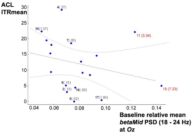
Figure 7. Scatterplot of baseline resting state relative mean betaMid PSDs at Oz vs. ITR_Mean in condition (i) ACL algorithm, 95% confidence regression bands as dotted lines, subject numbers in bold, Mahalanobis distances in brackets calculated in a linear regression analysis with the ITR_Mean as criterion variables and relative mean betaMid PSDs as predictor variables. Subject 15 and 11 (in red) might be considered as outliers (see text). Excluding them changes the Pearson correlation from r = −0.262, p = 0.294 to significant r = −0.510, p = 0.043.

Interestingly, excluding case 15 and 11, baseline resting state relative mean PSDs betaMid vs. thetaHigh both at Oz show an almost significant correlation over the subjects with r = −0.482 and p = 0.059, probably due to the small sample size, which is stable against the third variables age and all SSVEP-SNRs in the previous scanning phase of the experiment (a), (b), and (c), mentioned above.

In conclusion, baseline resting state relative mean betaMid PSDs seem to predict ITR performances under (i) ACL algorithm vs. (iii) top in an opposed fashion depending on the electrodes: the lower baseline resting state relative mean betaMid PSDs are at Oz, the higher will be the ITRs under condition (i); and the higher baseline resting state relative mean betaMid PSDs are at frontal electrodes (F3, Fz, F4) the higher will be the ITRs under condition (iii). In addition to these findings in betaMid, the higher the baseline resting state relative mean thetaHigh PSDs at Oz are, the higher will be the ITRs exclusively under condition (i).

Returning to the above described subsample of N = 12 obtained by exclusion of all subjects with N_Trials < 25th percentile (8.75 ≈ 9), an interesting observation was found: IAF shows differentiating relationships with ITR performances: a significant correlation of r = 0.577, p = 0.0496 was only found with ITRs under (i) ACL algorithm (see scatterplot Figure 8), but neither under (ii) top with r = 0.394, p = 0.205 nor under (iii) prefixed r = 0.283, p = 0.373. The higher subjects' IAF are in the subsample, the better will be their ITR performance exclusively under the ACL algorithm. Partial correlation analyses confirmed that this association is linearly independent against age. Repeating this analysis for the entire sample of N = 18 no significant correlations between individual alpha frequency (IAF) and ITR performances under the three experimental conditions become apparent (i) with r = 0.282, p = 0.257, (ii) r = 0.198, p = 0.432 and (iii) r = 0.243, p = 0.332. These findings imply that subjects with low ITRs in all three conditions might represent another population as compared to the rest. Further studies may try to replicate these findings and identify dimensions which discriminate between these possible two different populations. Moreover, these findings could be relevant for the understanding of the so-called BCI illiteracy phenomenon (Blankertz et al., 2010; Vidaurre and Blankertz, 2010; Volosyak et al., 2011), see section “Discussion.”

FIGURE 8

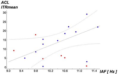
Figure 8. Scatterplot of individual alpha frequency (IAF) vs. ITR_Mean under condition (i) ACL algorithm (best-fit regression line for N = 12 as continuous line, 95% confidence regression bands as dotted lines). A significant Pearson correlation with r = 0.577, p = 0.0496 was found in the remaining subsample of N = 12 (blue points), removing subjects with N_Trials < 25th percentile (8.75 ≈ 9) (red points), while over the entire sample of N = 18 the correlation is hidden with r = 0.282, p = 0.257 (all points). This relationship seems to exist exclusively for condition (i) ACL algorithm: the higher subjects' IAF are in this subsample, the better will be their ITR_Mean performance exclusively under (i). Partial correlation analyses confirmed that this association is linearly independent against age.

Inspired by the findings of Koch et al. (2008) who found correlations of IAF with both magnitudes of visually evoked potentials (VEPs) and also with cortical oxygenation measured by near-infrared spectroscopy (NIRS), Spearman rank order correlations were computed between IAF and means of SSVEP-SNR magnitudes in the scanning phase of the experiment (a) over all 20 used flicker frequencies 20–39 Hz, (b) over the lower frequencies 20–29 Hz and (c) over the higher frequencies 30–39 Hz in the described subsample of N = 12. Although not fully reaching significance level, probably due to the relatively small sample size, an interesting pattern was found: IAF vs. (a) with rho = 0.561, p = 0.058, IAF vs. (b) with rho = 0.183, p = 0.568 and IAF vs. (c) rho = 0.557, p = 0.060. Although not fully significant, probably due to the small sample size, interindividual differences in SSVEP-SNR magnitudes under the employed higher flicker frequencies seem to show a tendency of positive association to higher IAFs while this relationship might not exist for the stimulation with the lower frequencies (or if so, it may presumably be lower). These findings motivated the re-analysis of the found relationship in Figure 8 by partial correlations whether it would be linearly independent against SSVEP-SNR magnitudes in the scanning phase of the experiment (a), (b) and (c) as described above. While (a) and (b) showed no relevant influence on this relationship, controlling for (c) resulted in a reduction from former Pearson r = 0.577, p = 0.0496 to r = 0.396, p = 0.228. Hence, these findings imply that IAF and (c) the magnitude of SSVEP responses to only the employed higher flicker frequencies share remarkably amounts of common interindividual variability while explaining variability of ITR_Mean under the ACL algorithm.

Effects of the Permutation of Presentation Order

Investigating possible effects of the permutation of presentation order, a mixed-design repeated measures ANOVA was computed with stimulation condition as repeated within-subjects factor with three levels (i) ACL algorithm represented as ITR_Median, (ii) prefixed and (iii) top and presentation order as between-subjects factor with the six possible permutations as levels (ABC, ACB, BAC etc.). Levene's tests showed homogeneities of error variances. There was no significant between-subjects main effect of presentation order with F_{(5, 18)} = 2.26, p = 0.115, η²_p = 0.485. Because Mauchly's sphericity test indicated a significant departure from the assumption of sphericity with χ² (2) = 6.54, p = 0.038, Greenhouse-Geisser estimates were used to correct degrees of freedom (ε = 0.691). There was no significant interaction between presentation order × stimulation condition with F_{(10, 18)} = 0.67, p = 0.738, η²_p = 0.219. ANOVA analyses were repeated also for condition (i) ACL algorithm represented as ITR_Mean and ITR_Max which resulted in similar findings. In conclusion, neither significant main effects nor significant interactions could be found over all six possible permutations of presentation order. Hence, the found effects in the central tendencies reported above with regard to all ITR performances can be considered as independent from possible presentation order effects.

Discussion

Although electrophysiology-based closed-loop interactions with biological nervous systems have been used since the 1940s, modern computers and online software control techniques allow a wide variety of novel activity dependent protocols in neuroscience research and related applications. Current BCI bring up a number of problems related to relatively long previous training times and still relatively low efficiencies (ITRs). This calls for novel techniques which can also address context and subject specificities, e.g., adaptive detection of SSVEPs (e.g., Krauledat et al., 2008).

In this paper we described an assisted closed-loop protocol which enhances BCI efficiency, as compared to classic BCI protocols, by providing both the subject and the system with online information which helps them to reach the BCI goal in their interaction. We used a reductionistic paradigm to constrain the inherent complexity of closed-loop exploration: four simultaneous frequencies, a basic SSVEP detection strategy and a relatively simple task to be accomplished by the user. More complex BCI systems might further benefit from the described approach. Our paradigm calls for many possible improvements, ranging from advanced SSVEP detection algorithms, stimuli which inform the user more effectively, up to a more adaptive online control of the interface itself by measuring and exploring additional dimensions (multimodality).

The literature on SSVEP-BCIs does not report general recommendations for the selection of the properties of the visual stimuli (Wu et al., 2008; Zhu et al., 2010), although it is known that the SSVEP magnitudes depend on extrinsic and intrinsic dimensions (Ding et al., 2006; Lopez-Gordo et al., 2011). Our study shows that a closed-loop subject-specific selection of the stimulation frequencies together with the closed-loop auditory feedback lead to increased BCI ITR performance which outperformed the employed control conditions.

Although assisted closed-loop protocols seem to enhance BCI efficiency, their use is limited by the additional time needed for the exploration process. In the protocol discussed in this paper, the average time to perform the experiment was around half an hour, flicker frequency selection took most of this time. Due to time restrictions, the parameter space can never be explored completely, so BCI efficiency improvement might remain suboptimal. Thus, there is some unknown trade-off between improvement and time needed, which should be explored in further studies. Furthermore, the question how replicable the found flicker frequencies are in the same subjects over multiple follow-up time points could be explored. Probably, observing this stability over time (e.g., test-retest reliability) may help to discover important trait vs. state dimensions related to variability of BCI performance. Another limitation due to the SSVEP physiology is that the time window for the auditory feedback is relatively short, so subjects have to establish control over the BCI goal in the range of a few seconds. This implies possible interactions with subjects' traits and states related to cognitive processing speed and dimensions of learning abilities.

ACL algorithms offer new possibilities as compared to traditional open-loop paradigms, but require additional decisions and new perspectives for their design and analysis, e.g., with regard to online measurement of actual states and performance, parameter search responding to the particular dynamic behavior of the system, properties of the feedback stimuli, actuation laws, etc. However, our findings imply that this additional effort can improve BCI efficiency and contribute to reveal dynamics of the nervous system which would remain hidden under traditional paradigms. Because our analyses showed that EEG resting state measures can predict assisted closed-loop SSVEP-BCI performance, our novel approach seems to flexibly adapt/interact with interindividual cerebral variabilities. Although found in the context of a sensory motor rhythms (SMRs) based BCI, other recent work also demonstrated that EEG resting state measures can be relevant predictors of BCI performance (Blankertz et al., 2010). In this emerging field, it could be fruitful to identify possible EEG resting state measures which can differentiate/predict between BCI performances based on biosignals originating from distinct physiological mechanisms: SSVEPs, P300, SMRs, slow cortical potentials (SCPs), electrocorticogram (ECoG), magnetoencephalography (MEG), NIRS or blood-oxygen-level-dependent (BOLD). Apart from these biosignals reflecting brain activity, peripheral psychophysiological measures have been investigated in the context of BCIs, especially as performance predictors, such as parasympathic/vagal parameters of resting state heart rate variability (HRV) (Kaufmann et al., 2011).

Our proposed approach of new adaptive-interactive paradigms might offer innovative ways how to address the problem of the so-called BCI illiteracy, i.e., the incapacity of some subjects to achieve control of BCIs (Blankertz et al., 2010; Vidaurre and Blankertz, 2010; Volosyak et al., 2011). It might be fruitful to explore the possible different impact of ACL algorithms in BCIs based on the mentioned distinct physiological mechanisms, especially with regard to their specific BCI illiteracies.

As mentioned in section “Baseline Resting State EEG Measures as Possible Interindividual Correlates of ITR Performances,” the IAF is a measure of interindividual EEG variability because it is remarkably stable within subjects, but relatively variable between subjects (Kondacs and Szabó, 1999). IAF seems to be highly heritable, e.g., Posthuma et al. (2001) found in a study comparing mono- vs. dizygotic twins, analyzing a large representative sample of healthy Dutch adults (N = 688), that 71–83% of total IAF variance could be ascribed to genetic variances. Thus, IAF may be considered as an endophenotype following the definition of Gottesman and Gould (2003). Klimesch (1997) found in a sample of age matched subjects that the IAF of good working memory performers is about 1 Hz higher vs. that of bad performers. Jin et al. (2006) found that IAF is positively correlated with conflict reaction time. Severity of Alzheimer's disease is positively related to the extent of typical IAF slowing in this pathology (Rodriguez et al., 1999). On the neurophysiological level, Steriade et al. (1990) reported that IAF depends on membrane properties of the thalamic neurons which project to the cortex, implying thalamo-cortical feedback loops as one of the important generators of alpha activity (Lopes da Silva, 1991). Mayer et al. (2007) successfully modeled the synchronization of locally coupled bistable thalamic oscillators as controlled by the influence of corticothalamic projections, probably responsible for widespread spindle oscillations in the thalamus. Given these findings, IAF might be understood as a positive correlate of thalamo-cortical information processing speed. With regard of possible correlations of IAF with SSVEP magnitudes, Koch et al. (2008) found interesting correlations of IAF with both magnitudes of VEPs and cortical oxygenation measured by NIRS. Concluding, IAF seems to open new insights into the understanding of the neural circuits underlying BCI performance and thus should be considered as a promising predictor for further studies.

In this study, only eight EEG electrodes were used to investigate EEG resting state measures as performance predictors, but further works might use more electrodes of the 10–20 system to allow a-posteriori offline analyses of scalp maps and the use of source localization techniques, e.g., LORETA (for a review see Grech et al., 2008). Findings of research concerning the cerebral resting-state networks call for further studies which use simultaneous EEG/fMRI recordings (for reviews see e.g., Fox and Raichle, 2007; Van den Heuvel and Hulshoff-Pol, 2010; for typical studies see e.g., Damoiseaux et al., 2006; Van den Heuvel et al., 2009; Yuan et al., 2012).

Opening the scope to other uses, the demonstrated advantage of our adaptive-interactive BCI protocol can be expanded conceptually, e.g., to innovative applications such as diagnostic/therapeutic tools in clinical contexts: exploring the subject-specific dynamical trajectory of machine-subject interaction could extract information which otherwise would remain undiscovered. Thus, far beyond an engineering focus, the proposed approach might be employed as a new paradigm for basic neuroscientific and biomedical research.

Conflict of Interest Statement

The authors declare that the research was conducted in the absence of any commercial or financial relationships that could be construed as a potential conflict of interest.

Acknowledgments

We thank Víctor Bonilla for technical help. This work was supported by UAM CEMU 2012-004, MINECO TIN2012-30883 and TIN-2010-19607.

References

Bayram, A., Bayraktaroglu, Z., Karahan, E., Erdogan, B., Bilgic, B., Ozker, M., et al. (2011). Simultaneous EEG/fMRI analysis of the resonance phenomena in steady-state visual evoked responses. Clin. EEG Neurosci. 42, 98–106.

Pubmed Abstract | Pubmed Full Text | CrossRef Full Text

Birbaumer, N. (2006). Breaking the silence: brain-computer interfaces (BCI) for communication and motor control. Psychophysiology 43, 517–532.

Pubmed Abstract | Pubmed Full Text | CrossRef Full Text

Blankertz, B., Sannelli, C., Halder, S., Hammer, E. M., Kübler, A., Müller, K.-R., et al. (2010). Neurophysiological predictor of SMR-based BCI performance. Neuroimage 51, 1303–1309.

Pubmed Abstract | Pubmed Full Text | CrossRef Full Text

Capilla, A., Pazo-Alvarez, P., Darriba, A., Campo, P., and Gross, J. (2011). Steady-state visual evoked potentials can be explained by temporal superposition of transient event-related responses. PLoS ONE 6:e14543. doi: 10.1371/journal.pone.0014543

Pubmed Abstract | Pubmed Full Text | CrossRef Full Text

Chamorro, P., Levi, R., Rodriguez, F. B., Pinto, R. D., and Varona, P. (2009). Real-time activity-dependent drug microinjection. BMC Neuroscience 10:P296. doi: 10.1186/1471-2202-10-S1-P296

CrossRef Full Text

Chamorro, P., Muñiz, C., Levi, R., Arroyo, D., Rodríguez, F. B., and Varona, P. (2012). Generalization of the dynamic clamp concept in neurophysiology and behavior. PLoS ONE 7:e40887. doi: 10.1371/journal.pone.0040887

Pubmed Abstract | Pubmed Full Text | CrossRef Full Text

Cohen, J. (1988). Statistical Power Analysis for the Behavioral Sciences. 2nd Edn. Hillsdale, NJ: Erlbaum.

Cole, K. S. (1955). “Ions, potentials and the nerve impulse,” in Electrochemistry in Biology and Medicine, ed T. Shedlovsky (New York, NY: Wiley), 121–140.

Conover, W. J. (1980). Practical Nonparametric Statistics. 2nd Edn. New York, NY: John Wiley and Sons.

Damoiseaux, J. S., Rombouts, S. A. R. B., Barkhof, F., Scheltens, P., Stam, C. J., Smith, S. M., et al. (2006). Consistent resting-state networks across healthy subjects. Proc. Natl. Acad. Sci. U.S.A. 103, 13848–13853.

Pubmed Abstract | Pubmed Full Text | CrossRef Full Text

Destexhe, A., and Bal, T. (eds.). (2009). Dynamic-Clamp: From Principles to Applications. New York, NY: Springer.

Diez, P. F., Mut, V., Laciar, E., and Avila, E. (2010). A comparison of monopolar and bipolar EEG recordings for SSVEP detection. Conf. Proc. IEEE Eng. Med. Biol. Soc. 2010, 5803–5806.

Pubmed Abstract | Pubmed Full Text | CrossRef Full Text

Diez, P. F., Mut, V. A., Avila-Perona, E. M., and Laciar-Leber, E. (2011). Asynchronous BCI control using high-frequency SSVEP. J. Neuroeng. Rehabil. 8:39. doi: 10.1186/1743-0003-8-39

Pubmed Abstract | Pubmed Full Text | CrossRef Full Text

Ding, J., Sperling, G., and Srinivasan, R. (2006). Attentional modulation of SSVEP power depends on the network tagged by the flicker frequency. Cereb. Cortex 16, 1016–1029.

Pubmed Abstract | Pubmed Full Text | CrossRef Full Text

Economo, M. N., Fernandez, F. R., and White, J. A. (2010). Dynamic clamp: alteration of response properties and creation of virtual realities in neurophysiology. J. Neurosci. 30, 2407–2413.

Pubmed Abstract | Pubmed Full Text | CrossRef Full Text

Faul, F., Erdfelder, E., Lang, A.-G., and Buchner, A. (2007). G^*Power 3: a flexible statistical power analysis program for the social, behavioral, and biomedical sciences. Behav. Res. Methods 39, 175–191.

Pubmed Abstract | Pubmed Full Text

Fox, M. D., and Raichle, M. E. (2007). Spontaneous fluctuations in brain activity observed with functional magnetic resonance imaging. Nat. Rev. Neurosci. 8, 700–711.

Pubmed Abstract | Pubmed Full Text | CrossRef Full Text

Funahashi, S. (2001). Neuronal mechanisms of executive control by the prefrontal cortex. Neurosci. Res. 39, 147–165.

Pubmed Abstract | Pubmed Full Text | CrossRef Full Text

Goaillard, J.-M., and Marder, E. (2006). Dynamic clamp analyses of cardiac, endocrine, and neural function. Physiology (Bethesda) 21, 197–207.

Pubmed Abstract | Pubmed Full Text | CrossRef Full Text

Gottesman, I. I., and Gould, T. D. (2003). The endophenotype concept in psychiatry: etymology and strategic intentions. Am. J. Psychiatry 160, 636–645.

Pubmed Abstract | Pubmed Full Text | CrossRef Full Text

Grech, R., Cassar, T., Muscat, J., Camilleri, K. P., Fabri, S. G., Zervakis, M., et al. (2008). Review on solving the inverse problem in EEG source analysis. J. Neuroeng. Rehabil. 5:25. doi: 10.1186/1743-0003-5-25

Pubmed Abstract | Pubmed Full Text | CrossRef Full Text

Grissom, R. J. (1994). Probability of the superior outcome of one treatment over another. J. Appl. Psychol. 79, 314–316.

Grissom, R. J., and Kim, J. J. (2012). Effect Sizes for Research: Univariate and Multivariate Applications. 2nd Edn. New York, NY: Routledge.

Harris, F. J. (1978). On the use of windows for harmonic analysis with the discrete Fourier transform. Proc. IEEE 66, 51–83.

Herrmann, C. S. (2001). Human EEG responses to 1-100 Hz flicker: resonance phenomena in visual cortex and their potential correlation to cognitive phenomena. Exp. Brain Res. 137, 346–353.

Pubmed Abstract | Pubmed Full Text

Jasper, H. H. (1958). The ten-twenty electrode system of the International Federation. Electroencephalogr. Clin. Neurophysiol. 10, 370–375.

Pubmed Abstract | Pubmed Full Text

Jin, Y., O'Halloran, J. P., Plon, L., Sandman, C. A., and Potkin, S. G. (2006). Alpha EEG predicts visual reaction time. Int. J. Neurosci. 116, 1035–1044.

Pubmed Abstract | Pubmed Full Text | CrossRef Full Text

Kaufmann, T., Vögele, C., Sütterlin, S., Lukito, S., and Kübler, A. (2011). Effects of resting heart rate variability on performance in the P300 brain-computer interface. Int. J. Psychophysiol. 83, 336–341.

Pubmed Abstract | Pubmed Full Text | CrossRef Full Text

Khan, A., and Rayner, G. D. (2003). Robustness to non-normality of common tests for the many-sample location problem. J. Appl. Math. Decis. Sci. 7, 187–206.

Klimesch, W. (1997). EEG-alpha rhythms and memory processes. Int. J. Psychophysiol. 26, 319–340.

Pubmed Abstract | Pubmed Full Text

Koch, S. P., Koendgen, S., Bourayou, R., Steinbrink, J., and Obrig, H. (2008). Individual alpha-frequency correlates with amplitude of visual evoked potential and hemodynamic response. Neuroimage 41, 233–242.

Pubmed Abstract | Pubmed Full Text | CrossRef Full Text

Kondacs, A., and Szabó, M. (1999). Long-term intra-individual variability of the background EEG in normals. Clin. Neurophysiol. 110, 1708–1716.

Pubmed Abstract | Pubmed Full Text

Krauledat, M., Tangermann, M., Blankertz, B., and Müller, K.-R. (2008). Towards zero training for brain-computer interfacing. PLoS ONE 3:e2967. doi: 10.1371/journal.pone.0002967

Pubmed Abstract | Pubmed Full Text | CrossRef Full Text

Lopes da Silva, F. (1991). Neural mechanisms underlying brain waves: from neural membranes to networks. Electroencephalogr. Clin. Neurophysiol. 79, 81–93.

Pubmed Abstract | Pubmed Full Text

Lopez-Gordo, M. A., Prieto, A., Pelayo, F., and Morillas, C. (2011). Customized stimulation enhances performance of independent binary SSVEP-BCIs. Clin. Neurophysiol. 122, 128–133.

Pubmed Abstract | Pubmed Full Text | CrossRef Full Text

Marmont, G. (1949). Studies on the axon membrane; a new method. J. Cell. Physiol. 34, 351–382.

Pubmed Abstract | Pubmed Full Text

Mayer, J., Schuster, H. G., Claussen, J. C., and Mölle, M. (2007). Corticothalamic projections control synchronization in locally coupled bistable thalamic oscillators. Phys. Rev. Lett. 99, 068102.

Pubmed Abstract | Pubmed Full Text | CrossRef Full Text

Morgan, S. T., Hansen, J. C., and Hillyard, S. A. (1996). Selective attention to stimulus location modulates the steady-state visual evoked potential. Proc. Natl. Acad. Sci. U.S.A. 93, 4770–4774.

Pubmed Abstract | Pubmed Full Text

Muniz, C., Forlim, C. G., Guariento, R. T., Pinto, R., Rodriguez, F., and Varona, P. (2011). Online video tracking for activity-dependent stimulation in neuroethology. BMC Neuroscience 12:P358. doi: 10.1186/1471-2202-12-S1-P358

CrossRef Full Text

Muniz, C., Levi, R., Benkrid, M., Rodriguez, F. B., and Varona, P. (2008). Real-time control of stepper motors for mechano-sensory stimulation. J. Neurosci. Methods 172, 105–111.

Pubmed Abstract | Pubmed Full Text | CrossRef Full Text

Nicolas-Alonso, L. F., and Gomez-Gil, J. (2012). Brain computer interfaces, a review. Sensors 12, 1211–1279.

Pubmed Abstract | Pubmed Full Text | CrossRef Full Text

Posthuma, D., Neale, M. C., Boomsma, D. I., and De Geus, E. J. (2001). Are smarter brains running faster? Heritability of alpha peak frequency, IQ, and their interrelation. Behav. Genet. 31, 567–579.

Pubmed Abstract | Pubmed Full Text

Prinz, A. A., Abbott, L. F., and Marder, E. (2004). The dynamic clamp comes of age. Trends Neurosci. 27, 218.

Pubmed Abstract | Pubmed Full Text | CrossRef Full Text

Regan, D. (1989). Human Electrophysiology: Evoked Potentials and Evoked Magnetic Fields in Science and Medicine. New York, NY: Elsevier.

Robinson, H. P., and Kawai, N. (1993). Injection of digitally synthesized synaptic conductance transients to measure the integrative properties of neurons. J. Neurosci. Methods 49, 157.

Pubmed Abstract | Pubmed Full Text

Rodriguez, G., Copello, F., Vitali, P., Perego, G., and Nobili, F. (1999). EEG spectral profile to stage Alzheimer's disease. Clin. Neurophysiol. 110, 1831–1837.

Pubmed Abstract | Pubmed Full Text

Schaich, E., and Hamerle, A. (1984). Verteilungsfreie Statistische Prüfverfahren. Berlin: Springer.

Sharp, A. A., O'Neil, M. B., Abbott, L. F., and Marder, E. (1993). Dynamic clamp: computer-generated conductances in real neurons. J. Neurophysiol. 69, 992–995.

Pubmed Abstract | Pubmed Full Text

Steriade, M., Gloor, P., Llinás, R. R., Lopes de Silva, F. H., and Mesulam, M. M. (1990). Report of IFCN Committee on Basic Mechanisms. Basic mechanisms of cerebral rhythmic activities. Electroencephalogr. Clin. Neurophysiol. 76, 481–508.

Pubmed Abstract | Pubmed Full Text

Usakli, A. B., and Gurkan, S. (2010). Design of a novel efficient human-computer interface: an electrooculagram based virtual keyboard. IEEE Trans. Instrum. Meas. 59, 2099–2108.

Van den Heuvel, M. P., and Hulshoff-Pol, H. E. (2010). Exploring the brain network: a review on resting-state fMRI functional connectivity. Eur. Neuropsychopharmacol. 20, 519–534.

Pubmed Abstract | Pubmed Full Text | CrossRef Full Text

Van den Heuvel, M. P., Mandl, R. C. W., Kahn, R. S., and Hulshoff Pol, H. E. (2009). Functionally linked resting-state networks reflect the underlying structural connectivity architecture of the human brain. Hum. Brain Mapp. 30, 3127–3141.

Pubmed Abstract | Pubmed Full Text | CrossRef Full Text

Van Gerven, M., Farquhar, J., Schaefer, R., Vlek, R., Geuze, J., Nijholt, A., et al. (2009). The brain-computer interface cycle. J. Neural Eng. 6:41001. doi: 10.1088/1741-2560/6/4/041001

Pubmed Abstract | Pubmed Full Text | CrossRef Full Text

Vialatte, F.-B., Maurice, M., Dauwels, J., and Cichocki, A. (2010). Steady-state visually evoked potentials: focus on essential paradigms and future perspectives. Prog. Neurobiol. 90, 418–438.

Pubmed Abstract | Pubmed Full Text | CrossRef Full Text

Vidaurre, C., and Blankertz, B. (2010). Towards a cure for BCI illiteracy. Brain Topogr. 23, 194–198.

Pubmed Abstract | Pubmed Full Text | CrossRef Full Text

Volosyak, I., Cecotti, H., and Gräser, A. (2009). “Impact of frequency selection on LCD screens for SSVEP based brain-computer interfaces,” in Proceedings of the 4th International IEEE/EMBS Conference on Neural Engineering NER 09 (Antalya, Turkey), 706–713.

Volosyak, I., Valbuena, D., Luth, T., Malechka, T., and Gräser, A. (2011). BCI demographics II: how many (and what kinds of) people can use a high-frequency SSVEP BCI? IEEE Trans. Neural Syst. Rehabil. Eng. 19, 232–239.

Pubmed Abstract | Pubmed Full Text | CrossRef Full Text

Wu, Z., Lai, Y., Xia, Y., Wu, D., and Yao, D. (2008). Stimulator selection in SSVEP-based BCI. Med. Eng. Phys. 30, 1079–1088.

Pubmed Abstract | Pubmed Full Text | CrossRef Full Text

Yuan, H., Zotev, V., Phillips, R., Drevets, W. C., and Bodurka, J. (2012). Spatiotemporal dynamics of the brain at rest–exploring EEG microstates as electrophysiological signatures of BOLD resting state networks. Neuroimage 60, 2062–2072.

Pubmed Abstract | Pubmed Full Text | CrossRef Full Text

Zhu, D., Bieger, J., Garcia Molina, G., and Aarts, R. M. (2010). A survey of stimulation methods used in SSVEP-based BCIs. Comput. Intell. Neurosci. 2010:702357. doi: 10.1155/2010/702357

Pubmed Abstract | Pubmed Full Text | CrossRef Full Text

Zschocke, S., and Hansen, H.-C. (eds.). (2012). Klinische Elektroenzephalographie. Berlin/Heidelberg: Springer.