Potential roles of the interaction between model V1 neurons with orientation-selective and non-selective surround inhibition in contour detection

Introduction

At the level of individual neurons and neuronal population, center–surround interactions across the receptive fields (RFs) of neurons are regarded as the underlying physiological bases of visual information processing (Fitzpatrick, 2000; Alitto and Dan, 2010). Following the important discoveries on the RFs of the visual system in the beginning of the 1960s (Hubel and Wiesel, 1962), researchers have conducted extensive work trying to uncover the temporal-spatial properties and the corresponding functional roles of the RFs in visual processing. Numerous neurophysiological findings on macaque monkeys and cats (Allman et al., 1985; Knierim and van Essen, 1992; Li and Li, 1994; Kapadia et al., 1995, 2000; Nothdurft et al., 1999; Sceniak et al., 1999, 2002; Walker et al., 1999; Jones et al., 2001; Angelucci and Bressloff, 2006; Song and Li, 2008; Chen et al., 2013) have clearly shown that for most neurons in the primary visual cortex (V1), the stimulus placed within the non-classical receptive field (nCRF), an extensive peripheral region beyond the central classical receptive field (CRF), can strongly modulate (mainly inhibit) the spiking response to the stimulus placed within CRF, and in general, the surround modulation varies depending on the properties of stimulus, especially the feature contrasts between the regions of CRF and nCRF, such as orientation contrast (Knierim and van Essen, 1992; Li and Li, 1994; Walker et al., 1999), luminance contrast (Levitt and Lund, 1997; Kapadia et al., 1999; Sceniak et al., 1999, 2002; Song and Li, 2008; Chen et al., 2013), spatial frequency contrast (Knierim and van Essen, 1992; Li and Li, 1994; Walker et al., 1999), and phase contrast (Li and Li, 1994; Nothdurft et al., 1999; Xu et al., 2005; Shen et al., 2007; Song and Li, 2008; Song et al., 2010).

In particular, many physiological studies showed that most V1 neurons are selectively responsive to visual stimuli of a narrow range of orientations, i.e., the strength of surround inhibition reaches maximal when the surrounding stimulus shares the same orientation with the stimulus within the CRF, and decreases with the increasing of orientation contrast between the central and surrounding stimuli (Knierim and van Essen, 1992; Li and Li, 1994; Walker et al., 1999), which is normally called orientation-selective inhibition. In addition, there are also several studies indicating that for a sizable group of neurons in V1 of anesthetized macaque monkeys, the strength of inhibition is independent of the orientation contrast between the stimuli within and outside the CRF (Nothdurft et al., 1999), which is referred as to non-selective inhibition or general inhibition. Both neurons with orientation-selective and with non-selective surround inhibition have been found in V1 of monkeys (Knierim and van Essen, 1992; Nothdurft et al., 1999) and cats (Li and Li, 1994; Sengpiel et al., 1997; Chen et al., 2013). Similar neuron types were also found in the V1 area of awake macaques with natural scene images as stimuli (Guo et al., 2005). Considering the co-existing of the neurons with orientation-selective and with non-selective surround inhibition in area V1 of monkeys and cats, it has been proposed that the surround could be looked at as a combination of the phenomena of orientation-selective and non-selective inhibition (Nothdurft et al., 1999).

Besides the surround inhibition, the modulation type of facilitation (or excitation) in V1 has been also found by many physiological studies (Levitt and Lund, 1997; Kapadia et al., 1999; Sceniak et al., 1999, 2002; Song and Li, 2008). While surround inhibition is thought to be mainly useful for suppressing unwanted background configurations, excitatory interactions are regarded to be especially helpful in linking together collinear edge elements (Grigorescu et al., 2003; Tang et al., 2007). In addition, significant evidence suggests that the surround inhibition and facilitation could be dynamically modified by feedback connections from higher visual cortexes, e.g., V4, according to stimulus context (Angelucci and Bressloff, 2006; Fei-Fei et al., 2007; Greene and Oliva, 2009; Wolfe et al., 2011; Gilbert and Li, 2013; Chen et al., 2014). Such top-down modulation of neuronal responses in V1 contributes to enhance the weak figural signal and reduce background noise. In short, the full V1 mechanism involves the combined contribution of feedforward (or bottom-up), lateral and feedback (or top-down) connections to the CRF center and its surround of V1 neurons. However, it is still not fully understood how the visual system integrates the local V1 neuronal activities into organized structures such as object contours.

Along another line, a number of computational models of contextual influences and center–surround interactions exist (e.g., the various models reviewed by Zhaoping, 2011), some focusing on the underlying neural circuits (Li, 1998; Ross et al., 2000; Ursino and La Cara, 2004; Hansen and Neumann, 2008; La Cara and Ursino, 2008), and others on the phenomenological modeling (Grigorescu et al., 2003, 2004; Petkov and Westenberg, 2003; Papari et al., 2007; Tang et al., 2007). In particular, some recent studies proposed models for computer vision applications by introducing the new properties of visual system, such as the disinhibition receptive field of ganglion cells in retina (Wei et al., 2012), adaptive inhibition (Zeng et al., 2011), sparse coding in V1 (Spratling, 2013), and multi-feature based surround modulation (Yang et al., 2014).

In this paper we are especially concerned with the computational evaluation of the role of orientation-selective and non-selective surround inhibition in the specific task of contour detection, which is not only helpful to understand the biological mechanisms of structured information detection, but also very useful for developing efficient models for various computer vision applications such as contour-based object recognition (Papari and Petkov, 2011). Among various biological vision inspired models mentioned above, Petkov and his collaborators (Grigorescu et al., 2003, 2004; Petkov and Westenberg, 2003) proposed two models (called anisotropic inhibition and isotropic inhibition), which employ the orientation-selective or non-selective surround inhibition alone. Both models were shown to outperform the traditional algorithms such as Canny detector (Canny, 1986). However, as implied by the results of Grigorescu et al. (2003), orientation-selective and non-selective surround inhibitions show different detection performance in different texture patterns. To date, the different roles of the two types of surround inhibition have not been systematically evaluated from a computational point of view. The primary purpose of this work is to clarify how the two neuron types work interactively to better detect contours from cluttered scenes, which is expected to inspire efficient phenomenological models for engineering applications in field of computational machine-vision.

The rest of this paper is organized as follows. We first revisit the contour detection performance of the previous phenomenological models with non-selective inhibition and orientation-selective inhibition alone (Grigorescu et al., 2003; Tang et al., 2007). Based on the deduced specific roles of these two types of surround inhibition, we propose two integrated adaptive models, namely, Models 1 and 2, by combining the two inhibition types. We try to constrain the parameter settings of the proposed models by biological measurements wherever possible. We finally validate the proposed models on a natural image dataset commonly used in the field of computer vision applications.

Materials and Methods

The Mathematical Representations of CRF and nCRF

The receptive field (RF) properties of simple cells in V1 can be well-described by a family of Gabor filters (Daugman, 1985; Jones and Palmer, 1987; Morrone and Burr, 1988). In this study, a Gabor energy model, which combines the responses of the pairs of Gabor filters with orthogonal in phase, is used to simulate the response of complex V1 cells (Chan and Coghill, 2001).

A two-dimensional (2D) Gabor filter can be written as

$\begin{array}{cc}g(x,y;\theta ,\phi )=\frac{1}{2\pi {\sigma }^2}\exp \left(-\frac{{\tilde{x}}^2+{\gamma }^2{\tilde{y}}^2}{2{\sigma }^2}\right)\cos \left(2\pi \frac{\tilde{x}}{\lambda }+\phi \right).& (1)\end{array}$

where $\tilde{x}$ = x cos θ + y sin θ, ỹ = −x sin θ + y cos θ, in which θ is the preferred orientation of an orientation-selective V1 neuron. Standard deviation σ defines the spatial size of CRF. γ is the spatial aspect ratio determining the eccentricity of the Gaussian envelope. λ is the wavelength and σ/λ represents the spatial frequency bandwidth. In this study we set σ/λ = 0.56 and γ = 0.5, which are physiologically based (Grigorescu et al., 2003; Petkov and Westenberg, 2003; Zeng et al., 2011). φ is a phase offset, and typically, the filter is symmetric when φ = 0 or π and asymmetric when φ = −(π/2) or (π/2).

According to the physiological finding of Hubel and Wiesel (1962), we define that at each sampling location (x, y), there is a model V1 hypercolumn composed of cells whose CRFs are centered at (x, y) and tuned to N_θ different orientations θ_i spanning 180°:

$\begin{array}{cc}{\theta }_i=\frac{(i-1)\pi }{N_{\theta }},i=1,2,\cdots ,N_{\theta }.& (2)\end{array}$

For an input image f(x, y), the CRF response of a complex V1 cell to the stimulus placed at location (x, y) is computed according to the Gabor energy model, which is written as

$\begin{array}{cc}\begin{array}{l}E(x,y;{\theta }_i)=\sqrt{{\left[e_0(x,y;{\theta }_i)\right]}^2+{\left[e_{\pi /2}(x,y;{\theta }_i)\right]}^2}.\hfill \\ e_{\phi }(x,y;{\theta }_i)=f(x,y)\ast g(x,y;{\theta }_i,\phi ).\hfill \end{array}& (3)\end{array}$

where * denotes the convolution operation. e₀(x, y; θ_i) and e_π/2(x, y; θ_i) are the responses of symmetric (or even) and asymmetric (or odd) Gabor filters at orientation θ_i, respectively.

To quantify the neuronal behavior that the modulation strength coming from nCRF decreases non-linearly with the increased distance from the center of CRF, a distance related weighting function is defined as Grigorescu et al. (2003) and Zeng et al. (2011).

$\begin{array}{cc}{W}_d(x,y)=\frac{H({\text{DOG}}_{\sigma ,k}(x,y))}{{\Vert H({\text{DOG}}_{\sigma ,k}(x,y))\Vert }_1}.& (4)\end{array}$

$\begin{array}{cc}H(s)=\{\begin{array}{l}s,s\ge 0\hfill \\ 0,s<0\hfill \end{array}\hfill & (5)\end{array}$

where ||·||₁ denotes the L₁ norm. H (s) is used to guarantee that neuronal responses should not be negative. DOG_σ,k(x, y) is the commonly used difference of Gaussian (DOG) function written as

$\begin{array}{cc}\begin{array}{l}{\text{DOG}}_{\sigma ,k}(x,y)=\frac{1}{2\pi {(k\sigma )}^2}\exp \left(-\frac{x^2+y^2}{2{(k\sigma )}^2}\right)\\ -\frac{1}{2\pi {\sigma }^2}\exp \left(-\frac{x^2+y^2}{2{\sigma }^2}\right).\end{array}& (6)\end{array}$

where k is the size ratio of nCRF to CRF. In this study we set k = 4 based on the physiological finding that the spatial size of nCRF is typically 2–5 times (in diameter) larger than that of CRF (Li and Li, 1994; Nothdurft et al., 1999).

Revisiting of the Orientation-selective and Non-selective Inhibition Models

Overview of Previous Surround Inhibition Models

Based on the physiological findings mentioned above, two typical phenomenological models have been proposed by Petkov and his colleagues (Grigorescu et al., 2003; Petkov and Westenberg, 2003) to simulate the orientation-selective and non-selective inhibition for the specific task of contour detection, i.e., non-selective inhibition model (also called isotropic inhibition model) and orientation-selective inhibition model (also called anisotropic inhibition model). In the isotropic inhibition model, the surround suppression is independent of the orientation difference between the stimuli within and outside the CRF. In the anisotropic inhibition model of Grigorescu et al. (2003) and Petkov and Westenberg (2003), surround inhibition works only when the stimuli within and outside the CRF share the same orientation, which does not quite match the physiological findings as mentioned earlier. To reinforce its physiological plausibility, Tang et al. (2007) proposed a unified contour extraction model based on visual cortical mechanisms including recurrent spatial facilitation and (orientation-selective) surround inhibition, in which the surround inhibition varies according to the orientation contrast between the stimuli inside and outside the CRF. They analyzed the effects of orientation-selective surround inhibition alone, but did not compare with that of non-selective surround inhibition. In the following, we will briefly introduce the isotropic inhibition model of Grigorescu et al. (2003) and Petkov and Westenberg (2003) and the anisotropic inhibition model extracted from the full model of Tang et al. (2007) and compare the performance of the two surround inhibition types on a synthetic image.

For each location of an input image, a winner-take-all (WTA) strategy is used to select the neuron with the maximum CRF response across the N_θ cells with different preferred orientations, which is written as

$\begin{array}{cc}\tilde{E}(x,y)=\max \left\{E(x,y;{\theta }_i)|i=1,2,\dots ,N_{\theta }\right\}.& (7)\end{array}$

where Ẽ(x, y) is called the maximum Gabor energy map, and the corresponding optimal orientation map is given by

$\begin{array}{cc}\tilde{\theta }(x,y)={\theta }_j,j=\arg \max \left\{E(x,y;{\theta }_i)|i=1,2,\dots ,N_{\theta }\right\}.& (8)\end{array}$

In order to describe the influence of the orientation contrast between CRF and nCRF on the inhibition strength, an orientation contrast based weighting function is defined as Tang et al. (2007).

$\begin{array}{cc}{\text{W}}_{\Delta \theta }({\theta }_{CRF},{\theta }_{nCRF})=\exp \left(-\frac{{\theta }_{\Delta }^2}{2{\sigma }_{\Delta }^2}\right).& (9)\end{array}$

$\begin{array}{cc}{\theta }_{\Delta }=\{\begin{array}{l}|{\theta }_{CRF}-{\theta }_{nCRF}|,|{\theta }_{CRF}-{\theta }_{nCRF}|<\pi /2\hfill \\ \pi -|{\theta }_{CRF}-{\theta }_{nCRF}|{,}_{|}{\theta }_{CRF}-{\theta }_{nCRF}|\ge \pi /2\hfill \end{array}& (10)\end{array}$

where θ_CRF and θ_nCRF are the orientations of the stimuli placed in CRF and nCRF, respectively, θ_Δ is the orientation contrast between θ_CRF and θ_nCRF. The standard deviation σ_Δ establishes a non-linear decreasing of the inhibition strength with the increasing of orientation contrast. We experimentally set σ_Δ = π/6 in this study.

The orientation-selective (OS) inhibition I_os(x, y) is computed at each location

$\begin{array}{cc}\begin{array}{l}{I}_{os}(x,y)={\displaystyle \sum _{(m,n)}{\text{W}}_{\Delta \theta }}(\tilde{\theta }(x,y),\tilde{\theta }(x+m,y+n))·\\ W_d(m,n)·\tilde{E}(x+m,y+n).\end{array}& (11)\end{array}$

Note that on the right-hand-side of above equation, we take the summation across all the locations around (x, y) that meet (x + m, y + n) ∈ R_nCRF, where R_nCRF represents the nCRF region.

In contrast, the non-selective (NS) inhibition term I_ns(x, y) is independent of the orientation contrast, which can be modeled by convoluting the Gabor energy Ẽ(x, y) with the spatial weighting function W_d(x, y)

$\begin{array}{cc}{I}_{ns}(x,y)=\tilde{E}(x,y)\ast W_d(x,y).& (12)\end{array}$

Therefore, the final neuronal responses produced by the orientation-selective and non-selective model can be respectively written as

$\begin{array}{cc}{r}_{os}(x,y)=H(\tilde{E}(x,y)-\alpha ·I_{os}(x,y)).& (13)\end{array}$

$\begin{array}{cc}{r}_{ns}(x,y)=H(\tilde{E}(x,y)-\alpha ·I_{ns}(x,y)).& (14)\end{array}$

where H(·) is defined as in Equation (5), i.e., H(s) = s while s > 0 and H(s) = 0 while s ≤ 0. α is a parameter used to control the strength of surround inhibition.

We schematically draw in Figure 1 the possible local neural networks of V1 cells with orientation-selective and with non-selective surround inhibition. Note that physiologically, the inhibition of surrounding excitatory neurons to the excitatory neurons in CRF is realized via additional inhibitory interneurons (Li, 1998; Fitzpatrick, 2000; Alitto and Dan, 2010). Here we omit such interneurons for graphical clarity, and simplify each inhibitory route as a short- or long-range synapse. In Figure 1A, the cell with orientation-selective surround inhibition receives different synaptic strengths depending on the orientation difference between the central and surrounding stimuli. In contrast, the cell with non-selective surround inhibition receives same synaptic strengths regardless of the orientation contrast (Figure 1B).

FIGURE 1

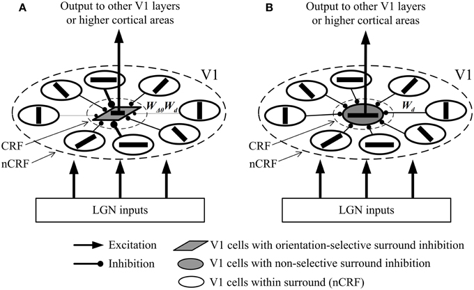
Figure 1. Simplified possible neural networks of surround inhibition mechanisms of the two types of V1 neurons. Here a cortical excitatory neuron in CRF only receives the feed-forward LGN input and feed-forward inhibition coming from the neighboring inhibitory interneurons that are activated by the excitatory neurons in nCRF via lateral connections (Fitzpatrick, 2000; Alitto and Dan, 2010). Note that the interneurons are not shown for the sake of graphical clarity, and the excitatory neurons in nCRF (namely, the pre-synaptic cells) connect directly to the excitatory neurons in CRF (namely, the post-synaptic cells). W_d is a weighting controlled by the distance between the pre-synaptic and post-synaptic cells. (see Equation 4), and W_Δθ is a weighting determined by the angle difference between the preferred orientations of the pre-synaptic and post-synaptic cells. (see Equation 9). (A) The local network of a V1 cell with orientation-selective surround inhibition. The synaptic strength of inhibition depends on both W_Δθ and W_d. (B) The local network of a V1 cell with non-selective surround inhibition. The synaptic strength of inhibition depends only on W_d. Different widths of the connection lines signify different synaptic strengths: thicker lines denote stronger (inhibitory) synapses. For example, the lengths of different connections in (B) are equal, which results in the same widths of the connection lines and the equal synaptic strengths (W_d).

Performance Evaluation of Surround Inhibition Based Models

The models mentioned above have been tested with synthetic and natural images (Grigorescu et al., 2003; Tang et al., 2007) and the results showed that both models exhibit better performance than traditional edge detectors such as Canny for contour detection and texture suppression. To conclusively identify the different roles of these two inhibition mechanisms in contour detection, here we first re-evaluated them with a synthetic image (Figure 2), in which a salient line (contour) is embedded in four different kinds of backgrounds [see regions (i–iv) of Figure 2A]. In particular, region (iii) is divided into small square areas with a size of 15 × 15 pixels. Each square contains a bar stimulus (10 pixels long and 2 pixels wide) with random orientation. Region (iv) contains a vertical line and a grating with an orientation of 45° from the vertical. The distance between any two neighboring black lines of the grating is 15 pixels.

FIGURE 2

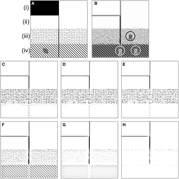
Figure 2. Results of the orientation-selective inhibition operator and non-selective inhibition operator on the synthetic map. (A) There are four kinds of backgrounds [i.e., (i)–(iv)] included in the image. The inset of the ellipse-shaped Gabor filter on region (iv) illustrates the preferred frequency of CRF compared to that of the grating element. (B) The maximum Gabor energy map. The concentric circles denoting the DOG-shaped RF (CRF plus nCRF) illustrates the relative size of the RF compared to the stimulus element. Point P1 is on the salient line segment embedded in the grating texture, P2 locates in the cluttered texture, and P3 is in the grating texture. Note that darker pixels correspond to higher neuronal responses, which holds for (C–H). (C–E) are the final responses of the orientation-selective inhibition operator with three different inhibition strengths: α = 1.6, 1.8, and 2.0, respectively (Equation 13). It is clear that the salient segment in randomly oriented textures [e.g., the region (iii) where point P2 locates] has no chance to pop out with the mechanism of orientation-selective inhibition. In contrast, the salient segment embedded in the uniformly orientated background [e.g., the region (iv) where point P1 and P3 locate] pops out easily. (F–H) are the final responses of non-selective inhibition operator with three different inhibition strengths: α = 0.8, 1.2, and 1.6, respectively (Equation 14). It is obvious that the salient segment in randomly oriented textures [e.g., the region (iii) where point P2 locates] pops out easily with the mechanism of non-selective inhibition. In contrast, the salient segment embedded in the uniformly orientated background [e.g., the region (iv) where point P1 locates] fades away when such type of surround inhibition works. See detailed analysis in the text.

We always set σ = 4.0 for the spatial size of the Gabor filter (Equation 1) when computing the CRF response (i.e., Gabor energy) to the stimuli in Figure 2A and for the scale of DOG filter [i.e., with the scales of 4.0 and 16.0 for the CRF and nCRF, respectively, see Equation (6)] when computing the surround inhibition based on the Gabor energy map (Figure 2B). According to the definition of Gabor and DOG+ functions in Section The Mathematical Representations of CRF and nCRF, the CRF region of a neuron covers about 2 bars and the surround (nCRF) covers about 5 × 5 bars in region (iii), and the CRF and nCRF may cover about 2 and 5 black lines of the grating in region (iv), as illustrated by the ellipse-shaped Gabor filter on Figure 2A and the DOG-shaped RF on Figure 2B.

The results shown in Figure 2 clearly demonstrate that both of the orientation-selective and non-selective inhibition models can easily extract the luminance edges [see region (i)] and isolated lines [see region (ii)], which is consistent with the results of other work (Grigorescu et al., 2003; Petkov and Westenberg, 2003). However, Figures 2C–E also illustrate that the orientation-selective inhibition operator has the remarkable ability to extract the salient line surrounded by a grating with different orientation [see region (iv)], but incapable for the salient line in the textural background with randomly oriented bars [see region (iii)]. More detailed analysis is as below. The salient line in region (iv) (e.g., see point P1 in Figure 2B) receives relatively weak surround inhibition, because there exists a orientation contrast of about 45° between the stimuli in CRF and nCRF in this specific case. In contrast, the grating texture (e.g., see point P3 in Figure 2B) receives strong surround inhibition since no orientation contrast exists between the stimuli in CRF and its surround. Therefore, cells with orientation-selective inhibition can reserve the contours in region (iv) and suppress the grating-shaped textural background. Note that the extracted salient segment in region (iv) is incomplete, which could be integrated using other mechanisms such as spatial facilitation (Grigorescu et al., 2003; Tang et al., 2007).

On the other hand, the texture in region (iii) (e.g., see point P2 in Figure 2B) receives relatively weak orientation-selective inhibition from surround due to the random orientation of the stimuli, and hence, the orientation-selective inhibition operator can not respond well to the salient lines merged in cluttered texture like region (iii). Figures 2C–E illustrate that the contour line and texture in region (iii) are always reserved or suppressed simultaneously when the inhibition strength (the factor α in Equation 13) varies.

The opposite situation occurs for the non-selective inhibition operator (Figures 2F–H), in which surrounding stimuli with same texture density would contribute equal inhibition strength to CRF, no matter the surrounding stimuli are uniformly or randomly oriented. Both the contours embedded in regularly oriented texture (e.g., point P1 in Figure 2B) and the unwanted textures (e.g., point P2 in Figure 2B) receive very strong inhibition, which means that the non-selective inhibition operator has the ability to suppress the cluttered texture [region (iii)] but can not well-reserve the lines merged in oriented grating [region (iv)]. In addition, Figures 2F–H indicate that the salient line in region (iv) can not be well-extracted by just adjusting the inhibition strength α of the non-selective inhibition model (see Equation 14).

In short, while the mechanism of non-selective suppression cannot well account for the phenomenon of orientation contrast pop-out, as indicated by our Figures 2F,G and the Figure 10 of Petkov and Westenberg (2003), here we also clearly demonstrated that orientation-selective suppression is incapable of making well-defined structures perceptible beyond the randomly oriented textures.

One may argue that with the commonly accepted neural computation mechanism of max-pooling (or winner-take-all) (Li, 1999; Carandini and Heeger, 2012), the salient vertical line in Figure 2A could be easily extracted by assuming that the stimulus at each location might excite both types of neurons. For example, among a pool of two types of neurons, a neuron with orientation-selective surround inhibition would produce higher response to the salient segment in region (iv), and hence this segment would pop out; and a neuron with non-selective surround inhibition would produce higher response to the salient segment in region (iii), which makes this segment pop out. However, it is easily found that with only winner-take-all mechanism, it is difficult to effectively suppress some kinds of background, such as the randomly oriented textures in region (iii), where neurons with orientation-selective inhibition produce higher responses.

The New Integrated Inhibition Models

Based on the computational analysis mentioned above, we speculate that V1 cells with orientation-selective and with non-selective surround inhibition work cooperatively when they extract visual features such as salient contours from complex natural scenes. To verify this prediction from a computational point of view, we propose two new integrated models for contour detection by combining the two surround inhibition mechanisms in two different ways. (i) Model 1: a binary orientation-saliency (BOS) map is defined to determine the surround inhibition type at each location, i.e., two types of neurons with different surround inhibition mechanisms are selectively activated according to the local orientation saliency. (ii) Model 2: a real-valued orientation-saliency (ROS) map is defined as a spatial weighting function to control the contribution of orientation-selective and non-selective inhibition to the neuronal responses at each location, i.e., neurons with both types of surround inhibition work at each location, but with different contributions.

Model 1

In Model 1, we suppose that two types of neurons with different surround inhibition mechanisms are selectively activated according to the local visual patterns. Figure 3A shows the networking architecture of Model 1. The lateral geniculate nucleus (LGN) inputs from orientation-salient regions (e.g., the grating on the left part of visual inputs in Figure 3) will selectively excite the V1 cells with orientation-selective surround inhibition; and in contrast, the stimuli from non-orientation-salient regions (e.g., the random bar filled region on the right part of visual inputs in Figure 3) will only activate the V1 cells with non-selective surround inhibition. The detailed implementation of Model 1 is as follows.

FIGURE 3

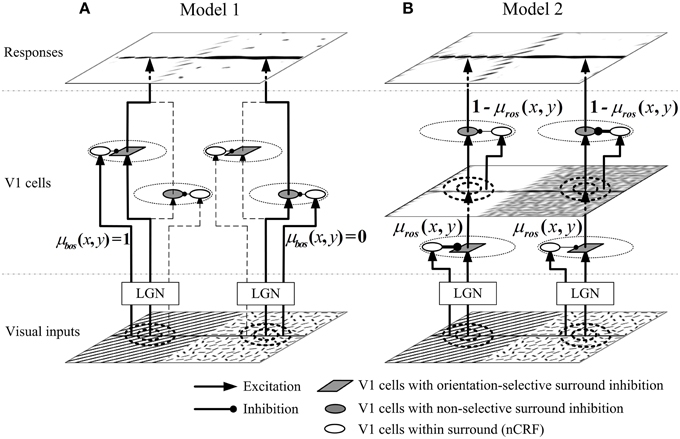
Figure 3. Networking structures of proposed models. (A) In Model 1, the orientation-salient regions (e.g., the grating on the left part of visual inputs, where μ_bos(x, y) = 1) is only processed by the V1 cells with orientation-selective surround inhibition; while the non-orientation-salient regions region (e.g., the random bar filled region on the right part of visual inputs, where μ_bos(x, y) = 0) is only processed by the V1 cells with non-selective surround inhibition. V1 cells on the branches of dashed lines are not selectively activated. (B) In Model 2, the input stimulus at each spatial location is first processed by the orientation-selective surround inhibition cells, and then processed by the non-selective surround inhibition cells. The ROS map μ_ros(x, y) (defined by Equation 15) determines the contribution of each type of cells at each location. For example, the orientation-salient region of grating receives stronger orientation-selective inhibition and weaker non-selective inhibition; the non-orientation-salient region of random bars is quite the reverse. The widths of the connections from the surrounding cells to CRF cells in Model 2 indicate the synaptic strengths: the thicker the connections, the stronger the synaptic strengths are.

In order to distinguish the different texture patterns based on local orientation features, we define μ_ros(x, y), the real-valued orientation-saliency (ROS) at spatial location (x, y), as a ratio of the maximum CRF response across all N_θ cells with different preferred orientations within a hypercolumn divided by the sum of CRF responses of these cells, which is given by

$\begin{array}{cc}{\mu }_{ros}(x,y)=\frac{\max \left\{E(x,y;{\theta }_i)\right\}}{{\displaystyle \sum _{i}E}(x,y;{\theta }_i)},i=1,2,\cdots ,N_{\theta }.& (15)\end{array}$

The computation of ROS according to Equation (15) could be realized by a neural network of divisive normalization shown in Figure 4. In the network a MAX-like operation is used to integrate the responses of V1 cells within a hypercolumn, which predicts the winner-take-all competition of cells in response to the input stimuli with different orientations. MAX-like computation has exhibited excellent capability in neural coding in V1 (Zhaoping and May, 2007) and IT (Riesenhuber and Poggio, 1999). Furthermore, the divisive normalization is considered as a canonical neural computation in the neural system (Carandini and Heeger, 2012).

FIGURE 4

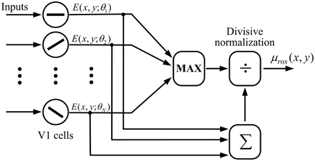
Figure 4. Computation of ROS with a possible neural network of divisive normalization. A winner-take-all (or MAX) operation is used to select the cell with the maximum CRF response across all N_θ cells with different preferred orientations within a hypercolumn, which is further divided by the sum of CRF responses of these cells.

An operation of Gaussian filtering is used to smooth μ_ros(x, y), and the whole ROS map is normalized to make μ_ros(x, y) ∈ [0, 1] for convenience. Then, a BOS map is calculated by binarizing the ROS map according to

$\begin{array}{cc}{\mu }_{bos}(x,y)=\{\begin{array}{l}1,{\mu }_{ros}(x,y)\ge th\hfill \\ 0,{\mu }_{ros}(x,y)<th\hfill \end{array}& (16)\end{array}$

where th is a threshold, and we experimentally set th = 0.4 in this study. Based on the BOS map, an input image is divided into orientation-salient regions (the regions with μ_bos(x, y) = 1) and non-orientation-salient regions (the regions with μ_bos(x, y) = 0). In the orientation-salient regions, only the neurons with orientation-selective surround inhibition are activated, and in contrast, neurons with non-selective inhibition work only in the non-orientation-salient regions.

The final neuronal response produced by Model 1 is given by

$\begin{array}{cc}{r}_1(x,y)=\{\begin{array}{l}H(\tilde{E}(x,y)-{\alpha }_1·I_{os}(x,y)),{\mu }_{bos}(x,y)=1\hfill \\ H(\tilde{E}(x,y)-{\alpha }_2·I_{ns}(x,y)),{\mu }_{bos}(x,y)=0\hfill \end{array}& (17)\end{array}$

where H(·) is an operator defined as in Equation (5), i.e., H(s) = s while s > 0 and H(s) = 0 while s ≤ 0. α₁ and α₂ are weighting factors to control the strengths of orientation-selective and non-selective surround inhibition.

For some simple images, such as the synthetic image shown in Figure 2A, the orientation-salient regions and non-orientation-salient regions can be easily and solely labeled using a BOS map and the contours can be effectively extracted using appropriate types of neurons. However, the following two reasons impel us to refine Model 1 in the next subsection: (1) the requirement of defining a suitable threshold value th (see Equation 16) seems non-biologically plausible and is not easy for each natural image; (2) most natural images are so complicated that uniformly and randomly oriented features always coexist in many local regions (Simoncelli, 2003; Olshausen and Field, 2004; Geisler, 2008; Tkaèik et al., 2010, 2011), which makes it not reasonable to simply define local regions as orientation-salient or non-orientation-salient.

Model 2

The general idea behind Model 2 is that each local region is always processed by both the neurons with orientation-selective and with non-selective surround inhibition (Figure 3B), and the relative contributions of the two types of neurons are controlled by the ROS map computed by Equation (15). For examples, orientation-salient regions (e.g., the grating on the left part of visual inputs in Figure 3) will be processed by stronger orientation-selective surround inhibition followed by weaker non-selective surround inhibition. Conversely, the stimuli from the non-orientation-salient regions (e.g., the random bar filled region on the right part of visual inputs in Figure 3) will be suppressed by weaker orientation-selective surround inhibition followed by stronger non-selective surround inhibition. The implementation details of Model 2 are as follows.

Considering the fact that non-selective surround inhibition may severely suppress the neuronal responses to the contours embedded in the uniformly oriented background (Figures 2F–H), the input image in Model 2 is first processed by neurons with orientation-selective inhibition, and the neuronal response is written as

$\begin{array}{cc}{R}_{os}(x,y)=H(\tilde{E}(x,y)-{\alpha }_1·{\mu }_{ros}(x,y)·I_{os}(x,y)).& (18)\end{array}$

where H(·) is defined as in Equation (5) to restrict neuronal responses non-negative. ROS map μ_ros(x, y) is used as a spatial weighting function. α₁ is a parameter used to control the synaptic strength of the orientation-selective surround inhibition. Equation (18) indicates that neurons at local regions with a higher orientation saliency would receive greater orientation-selective surround inhibition.

The output produced by Equation (18) contains randomly oriented features, which is further processed by the neurons with non-selective inhibition. The non-selective surround inhibition term R_ns(x, y) is easily computed by convoluting R_os(x, y) with the spatial weighting function W_d(x, y):

$\begin{array}{cc}{R}_{ns}(x,y)=R_{os}(x,y)\ast W_d\left(x,y\right).& (19)\end{array}$

The final response of the neurons simulated in Model 2 is given by

$\begin{array}{cc}{r}_2(x,y)=H(R_{os}(x,y)-{\alpha }_2·(1-{\mu }_{ros}(x,y))·R_{ns}(x,y)).& (20)\end{array}$

where α₂ is a parameter controlling the synaptic strength of the non-selective surround inhibition. Equation (20) indicates that in the regions with more randomly oriented features, neurons with non-selective inhibition would receive higher surround inhibition, which is scaled by 1 − μ_ros(x, y).

It should be clarified that the present Models 1 and 2 are computationally implemented using the Gabor-based phenomenological framework and the operation of convolution, but in fact, these models can be biologically plausibly explained and implemented using the form of neural circuits. The convolution of Gabor energy map with a weighting template (e.g., Equations 12 and 19) is in nature a simple implementation of summing the synaptic strength weighted modulation coming from the activated neurons in the nCRF region (Ursino and La Cara, 2004; La Cara and Ursino, 2008; Zeng et al., 2011), where the Gabor energy at each location denotes the spiking response of a V1 neuron and the value of the weighting template represents the strength of the feed-forward inhibitory synapse targeting the CRF neuron.

Experimental Results

The Performance of the Integrated Models on a Synthetic Image

To understand the behaviors of proposed models, we evaluated their performance with the synthetic image shown in Figure 5A. Figure 5B shows the maximum Gabor energy map corresponding to the input image, and the ROS map and BOS map are shown in Figure 5C and Figure 5D, respectively. From the results shown in Figure 5E we can clearly find that Model 1 responds well to isolated lines [e.g., in region (ii)] and luminance contrast edges [e.g., in region (i)], which were classified as orientation-salient regions (Figure 5D) and were detected by neurons with orientation-selective inhibition. In addition, Model 1 responds well to the organized lines embedded in the cluttered background, which were selectively extracted from orientation-salient regions [e.g., region (iv)] by neurons with orientation-selective inhibition or from non-orientation-salient regions [e.g., region (iii)] by neurons with non-selective inhibition. As shown in Figure 5E, all the meaningful edges mentioned above are clearly extracted while the oriented or cluttered backgrounds are effectively suppressed with Model 1.

FIGURE 5

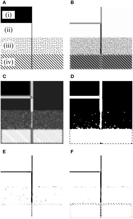
Figure 5. Results of our models on a synthetic image. (A) Input image with four kinds of backgrounds [i.e., (i–iv)]. (B) The maximum Gabor energy map [darker pixels correspond to higher neuronal responses, which holds for (E,F)]. (C) The real orientation-saliency (ROS) map defined by Equation (15) (whiter pixels correspond to higher orientation-saliencies). (D) The binary orientation-saliency (BOS) map defined by Equation (16) with th = 0.4 (white and black areas denote respectively the orientation-salient and non-orientation-salient regions). (E) The final output of Model 1 with α₁ = 1.60 and α₂ = 1.60. (F) The final output of Model 2 with α₁ = 1.60 (in Equation 18) and α₂ = 2.56 (in Equation 20).

On this synthetic image, Model 2 also provides excellent contour detection result (Figure 5F). In particular, Model 2 suppresses the cluttered background in region (iii) more completely than Model 1, due that Model 1 wrongly classifies a few local clusters in region (iii) as the orientation-salient, and the responses of the activated cells with orientation-selective inhibition to these clusters can not be sufficiently suppressed by the randomly oriented surrounding stimuli.

One may argue that if the contribution of facilitatory modulation to contour pop-out was introduced, it would be unnecessary to explicitly differentiate the roles of orientation-selective and non-selective surround inhibition, since both the two types of inhibition seem to work as noise eliminators. Figure 2A may serve as example to illuminate the important differences between the two types of inhibition. When responding to the stimuli in region (iv) of Figure 2A, the strengths of collinear facilitation are (almost) equal at all spatial locations, and meanwhile, the strengths of non-selective inhibition at all locations of this region are also equal. Hence, non-selective inhibition together with collinear facilitation can not make the vertical line segment in this region pop-out. In contrast, the type of orientation-selective inhibition (or together with collinear facilitation) can accomplish this visual task easily.

It should be pointed out that the boundary between the regions (ii) and (iii) and the boundary between the regions (iii) and (iv) can not be extracted and connected into clear and smooth contours by Models 1 or 2. The reason is mainly that these two boundaries are texture defined, and more visual features like frequency and phase contrasts and even higher cortical areas like V2 may be required to effectively detect such kind of edges (Li and Li, 1994; Nothdurft et al., 1999; Xu et al., 2005; Shen et al., 2007; Song and Li, 2008; Song et al., 2010).

Contour Detection on Natural Images

The performance was also tested with the widely used RuG dataset (Grigorescu et al., 2003; Papari et al., 2007; Tang et al., 2007; Papari and Petkov, 2008; Zeng et al., 2011), which includes 40 gray-level natural images and each has an associated ground-truth binary contour map drawn by a human (downloaded from http://www.cs.rug.nl/~imaging/databases/contour_database/contour_database.html). The performance of our models was compared with that of the typical orientation-selective and non-selective inhibition models proposed by Grigorescu et al. (2003), as described before.

In order to compare with the binary ground-truth contour map, the contour results extracted with different models were binarized using the standard procedure of non-maxima suppression followed by hysteresis thresholding (Canny, 1986; Grigorescu et al., 2003). In short, a non-maxima suppression operation was used to thin the candidate contours, and then an operation of hysteresis thresholding was applied to obtain the binary contour with one-pixel wide. Same as Grigorescu et al. (2003) and Zeng et al. (2011), we fixed t_Bl = 0.5t_Bh, where t_Bh and t_Bl are two parameters defining the low and high threshold values involved in the process of hysteresis thresholding. The details of non-maxima suppression and hysteresis thresholding could be referred to other literatures (Canny, 1986; Grigorescu et al., 2003).

We tested all the models with the same 80 groups of different parameter combinations in order to fully demonstrate their performance in a statistical manner. Specifically, we set N_θ = 12 for the Gabor filters. For the orientation-selective and non-selective inhibition models, we used eight scales of Gabor filters, σ ∈ {1.0, 1.2, 1.4, 1.6, 1.8, 2.0, 2.2, 2.4} and α ∈ {1.0, 1.2}. We applied five high hysteresis threshold values based on the percentage of candidate edge pixels with p ∈ {0.1, 0.2, 0.3, 0.4, 0.5}. For our models, we used four Gabor scales, σ ∈ {1.2, 1.6, 2.0, 2.4}, covering the most same domain of the Gabor filters as the eight scales mentioned above. We used α₁ ∈ {1.8, 2.0} and α₂ ∈ {1.2, 1.4} α₁ to control the strength of orientation-selective inhibition and non-selective inhibition, respectively; and p ∈ {0.5, 0.6, 0.7, 0.8, 0.9}, with same distribution range as other models considered here, for hysteresis threshold processing. Taken together with the results of Grigorescu et al. (2003) and our extensive testing, it is reasonable to propose that the 80 groups of parameter combinations obtained with these parameter settings are able to fairly exploit the overall performance of our models and other two existing models.

Qualitative Comparison

The best contour detection results among those obtained with the 80 groups of parameter combinations are compared in Figure 6 for four of total 40 RuG images. From the figure we can find that our Models 1 and 2 outperform the models with orientation-selective (denoted by OS) and non-selective (denoted by NS) inhibition alone, especially on the suppression of texture edges. In particular, we can clearly see that in the binary contour maps achieved by our Model 2 (the third rows in Figure 6), the extracted contours are smoother (with fewer cracks), with much fewer trivial edges on the images, which indicates that our Model 2 is capable of extracting salient contours and suppresses the texture edges (like foliage or grass) much more effectively than other models.

FIGURE 6

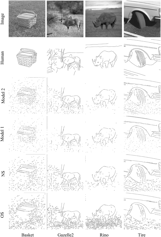
Figure 6. Comparison of contour detection results on real images. From top to bottom, rows show the four of the test images (the first row), their corresponding ground truth contour maps (the second row), the best contour maps obtained with our Model 2 (the third row) and Model 1 (the fourth row), and the best contour maps obtained with non-selective (denoted by NS) (the fifth row) and orientation-selective (denoted by OS) (the last row) inhibition models.

Quantitative Comparison

We measured the similarity of the output of computational models and the ground-truth contour map of each image. Generally, contours cannot always be detected at exact location. Following the work of Grigorescu et al. (2003), in this study, a 5 × 5 square neighborhood is used as a tolerance when matching a contour pixel in the algorithm output to the ground truth contours. That means a pixel detected by model is considered as correctly contour pixel if there is (at least) a ground truth contour pixel presenting in its 5 × 5 square neighborhood. Let E_GT and E_D be respectively the set of ground-truth contour pixels and pixels detected by a model. Then, the pixel set of correctly contour pixels detected by a model (denoted by E) is E = E_D ∩ (E_GT ⊕ T) (Note that ⊕ is the dilate operator and T is a 5 × 5 square template). The pixel set of false positives (denoted by E_FP) is determined by eliminating the correctly detected contour pixels from all pixels detected by model, i.e., E_FP = E_D − E. In contrast, the pixel set of false negatives (denoted by E_FN) is determined by eliminating those ground truth pixels, which present in the 5 × 5 square neighborhood of correctly detected contour pixels, from all ground truth contour pixels, i.e., E_FN = E_GT − (E_GT ∩ (E_D ⊕ T)). Then the percentage of false positives e_FP, the percentage of false negatives e_FN and the overall performance measure P could be computed according to Grigorescu et al. (2003), Tang et al. (2007), and Zeng et al. (2011)

$\begin{array}{cc}{e}_{FP}=\text{card}(E_{FP})/\text{card}(E).& (21)\end{array}$

$\begin{array}{cc}{e}_{FN}=\text{card}(E_{FN})/\text{card}(E_{GT}).& (22)\end{array}$

$\begin{array}{cc}P=\frac{\text{card}(E)}{\text{card}(E)+\text{card}(E_{FP})+\text{card}(E_{FN})}.\hfill & (23)\end{array}$

where card(S) represents the number of elements of the set S. It is obvious from the definitions that a lower e_FP, caused by the lower false positives and more correctly detected pixels, indicates a better suppression of textured background. Similarly, a lower e_FN means a better integrity of salient contour, and as a whole, a better overall performance results in a higher P.

Table 1 lists the best P and the corresponding parameter settings for the four images shown in Figure 6. The data clearly show that our Models 1 and 2 provide smaller e_FP, which quantitatively reveals that our two models exhibit excellent ability for suppressing texture edges. Meanwhile, our models obtain superior overall performance (higher P) by balancing the rate of false positive and false negative (lower e_FP and lower e_FN).

TABLE 1

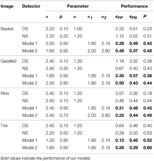
Table 1. Parameter settings and the best performance of different models.

Figure 7 illustrates the performance comparison of different models with the statistical box-and-whisker plots for the eight of 40 natural images. The top end of a whisker and the horizontal red line in the box represent respectively the best and the median P (denoted by P_max and P_med, respectively) among the 80 performance measures obtained with the 80 groups of parameter combinations. In our Model 2, the best performance P_max is substantially higher in comparison to that of the orientation-selective and non-selective inhibition models. In addition, our models produce a consistently higher median performance P_med than the two models with orientation-selective or non-selective inhibition alone.

FIGURE 7

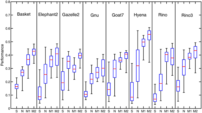
Figure 7. Box-and-Whisker statistical comparison of different models. The Box-and-Whisker plots compare the performance of the orientation-selective inhibition model (denoted by OS), non-selective inhibition model (denoted by NS), our Model 1 (denoted by M1) and Model 2 (denoted by M2) for eight of the total 40 images. Note that the box-and-whisker statistical analysis was done on all the 40 images of the RuG dataset, eight of which are listed here just for the space limitation.

Figure 8A compares the average values of P_max and P_med achieved by each model, computed on the all 40 images of RuG dataset. Our Model 2 outperforms the models with non-selective or orientation-selective inhibition alone in terms of both P_max and P_med statistics. Meanwhile, we also analyzed the distribution range of P over all parameter combinations. The average values of the length of boxes and whiskers were computed on each model, as shown in Figure 8B.

FIGURE 8

Figure 8. Full statistical comparison of different models. (A) The statistics of the max P (P_max) and median P (P_med) of the Box-and-Whisker statistics as shown in Figure 7. (B) The statistics of the length of whiskers (P_max − P_min) and the length of boxes. The statistics shown in (A,B) were computed on the Box-and-Whisker statistics of all the 40 images of the whole RuG dataset. The error bars indicate 95% confidence intervals.

The statistics of P_max could reflect a model's capacity to achieve best performance P on each image with optimal parameter settings. In contrast, the statistics of P_med and the length of boxes and whiskers could reflect a model's robustness with various non-optimal parameter settings. The obvious superior statistics of P_med and the length of boxes and whiskers produced by our modes, especially Model 2, indicates that suitable combining of orientation-selective and non-selective inhibition mechanisms endows a computational model with a higher chance to obtain a better contour detection result on each image. We believe that the statistics of P_med and the length of boxes and whiskers are more critical for a contour detection model due to the fact that for a real-time computer vision application under varying scenes, it is impracticable to use an exhaustive searching method to find the optimal model parameters for each input image.

Taken together with Figures 7, 8, it is reasonable to conclude that our two models with integrated surround inhibition mechanisms have the potential to achieve the best contour detection results with higher performance than the models with the orientation-selective or non-selective inhibition mechanism alone. Furthermore, our two models have the capacity to obtain a better result for each image in more robust ways when non-optimal parameters are set in the models.

Discussion

This work focuses on the functional roles of two specific types of surround inhibition of V1 cells. From a physiological point of view, the goal of this study is not to develop a contour detection model incorporated with the full V1 mechanisms including surround inhibition, spatial facilitation, feedback modulation from higher levels, temporal dynamics, etc. (Field et al., 1993; Fitzpatrick, 2000; Seriès et al., 2003; Ursino and La Cara, 2004; Vonikakis et al., 2006; Dakin and Baruch, 2009; Huang et al., 2009; Chen et al., 2014), but to clarify the different roles of orientation-selective and non-selective surround inhibition of V1 neurons in the specific task of extracting salient contours of objects from cluttered background. As the basis of this study, we demonstrated in the very beginning of this paper that, in general, V1 neurons with non-selective surround inhibition exhibit better overall performance measure due to its markedly superior ability in suppressing noised background. In contrast, V1 neurons with orientation-selective inhibition show relatively higher capacity to retain organized contours embedded in uniformly oriented background.

More importantly, based on the above computational analysis, we proposed two new integrated models (i.e., Models 1 and 2) for salient contour detection by combining the two types of surround inhibition in different ways. The results on a natural image dataset with contour ground-truth showed that both our Models 1 and 2 outperform substantially the models with orientation-selective or non-selective inhibition alone, which implies a cooperative way among different types of V1 neurons at least when extracting salient contours from cluttered natural scenes. Furthermore, the substantial superiority of Model 2 over Model 1 may at least suggest a reasonable hypothesis that regularly and randomly oriented background patterns co-exist with different amounts at most spatial locations of natural scenes, which may provide meaningful implications for natural stimulus based physiological experiments and computer vision oriented applications. Note that it is beyond the scope of this work to compare the performance of our new models with that of the state-of-the-art methods developed mainly for the purpose of engineering applications (e.g., Arbelaez et al., 2011), since our focus in this study is especially on providing support for the idea that neurons with different surround inhibition prefer working cooperatively rather than alone.

To the best of our knowledge, none of the existing models has explicitly modeled the different functional roles of orientation-selective and non-selective surround inhibition within an integrated model. The reason we emphasize the difference between the two types of surround inhibition is that they act quite differently, almost conversely, to a same stimulus pattern. For example, to a vertical straight line embedded in horizontally oriented grating, a V1 cell with orientation-selective surround inhibition responds strongly, and in contrast, a cell with non-selective inhibition responds quite weakly (when other mechanisms like spatial facilitation are omitted). Hence, we suggest that a V1 model explicitly taking into account the two types of surround inhibition will become more physiologically plausible and computationally feasible.

Though discriminating the different roles of the two types of surround inhibition mechanisms is of no doubt meaningful, and the two possible solutions proposed in this study for combining the two inhibition types seem to work well, there is still no direct evidence for (or against) our two proposals of integrating different surround inhibition types. Even so, we can see many interesting experimental findings that may provide indirect support to the physiological plausibility underlying our models. For example, as for the biological counterpart of BOS or ROS map, a most possible explanation is that the BOS or ROS map is a certain kind of “gist” extracted very rapidly via a nonselective pathway from very brief visual presentations (Rousselet et al., 2005; Wolfe et al., 2011). It has been proposed that compared to the capacity limited selective pathway for fine feature extraction, binding, and object recognition, the nonselective pathway can extract rapidly and efficiently from the entire scene some statistics of global coarse information including the distributions of basic visual attributes, such as texture and color, the spatial layout, etc (Sanocki, 2003; Rousselet et al., 2005). These sources of statistical and structural cues could be used to direct the resources of the selective pathway intelligently to refine the extraction of basic spatial structures like object contours (Fei-Fei et al., 2007; Greene and Oliva, 2009; Wolfe et al., 2011). Apparently, this possible scenario deserves further investigation. A recent physiological study (Chen et al., 2014) found that the onset of responses in V1 to global contours in a cluttered background is delayed relative to that seen in V4 (though the responses in both areas continue to evolve in parallel after that time). This supports the previous suggestion that feedback from higher areas may serve to dynamically gate horizontal connections within V1, which can modify V1 response properties according to stimulus context (and behavioral goal) and confer selectivity for more complex stimulus geometries (Gilbert and Li, 2013). These studies strongly suggest that feedback modulation from higher to lower visual areas plays a critical role in conscious perception of global forms (e.g., object contours). In fact, for the task of contour detection, several models have already been proposed trying to show how the top–down interactions operate to modulate local circuits within V1 for both contour enhancement and background suppression (Li, 1998; Zeng et al., 2011; Piëch et al., 2013).

One may argue our finding that better performance is achieved by the hierarchical processing in Model 2, i.e., the visual inputs to V1 are processed first by neurons with orientation-selective surround inhibition, and then by neurons with non-selective surround inhibition. As demonstrated by the detailed results and the analysis mentioned earlier, this specific hierarchical processing is computationally required to extract boundaries in regularly oriented textures [e.g., region (iv) in Figure 2], and reversing this hierarchical order will make the boundaries undetectable in regularly oriented background. The biological plausibility underlying Model 2 is perhaps related to the intrinsic organization of the pin-wheel-like-orientation columns in V1. It has been long recognized that in the V1 area of high mammals, neurons are organized in clusters with similar spatial summation properties, e.g., neurons with similar orientation preference are arranged in iso-orientation domains (IOD) around pin-wheel centers (PC), and the orientation tuning curve of the pin-wheel cells is shallower and broader than that of the domain cells in their CRFs (Bonhoeffer and Grinvald, 1991; Maldonado et al., 1997; Nauhaus et al., 2008). Recent studies (Hashemi-Nezhad and Lyon, 2012; Liu et al., 2013) further revealed that the orientation tuning of the suppression in the non-classical surround (i.e., nCRF) is sharper for IOD than for PC. That is, the neurons with orientation-selective surround inhibition are mostly in domain regions, and in contrast, the cells with non-selective (or widely tuned) surround inhibition locate mainly within the pinwheel centers. Inspired by these findings, we hypothesize that the neurons with non-selective inhibition in PC might integrate the information from the neurons with orientation-selective inhibition in IOD by short-range lateral connections between PC and IOD regions (Malach et al., 1993; Das and Gilbert, 1999; Yousef et al., 2001). A possible flow of information transmission in our Model 2 could be: the inputs from LGN are first processed by some neurons in the spreading region of domain, and then integrated and further processed by PC neurons with non-selective inhibition. It is of course required to validate such information flow by further physiological experiments, e.g., by comparing the response latency related to the surround suppression of PC and domain neurons.

Finally, it is necessary to comment on some possible future improvements of the proposed models. Considering the special role of collinear facilitation in visual processing and its successful applications in computational modeling, one of our further research directions is to integrate facilitatory surround modulation into our models, which is not only helpful to objectively evaluate the functional role of different V1 elements, but also beneficial to the application goal of reconstructing incomplete contours and extracting Gestalt edges. Furthermore, incorporating top-down feedback mechanisms into computational models with appropriate ways is of no doubt helpful to substantially improve the performance of contour extraction in cluttered scenes, which is an especially challenging but engrossing future direction since only little knowledge about feedback from higher cortical areas has been experimentally discovered (Gilbert and Li, 2013; Chen et al., 2014).

In conclusion, much remains to be investigated about the functional role and the underlying mechanisms of surround inhibition of V1 neurons in visual processing of natural scenes (Fitzpatrick, 2000; Alitto and Dan, 2010). The computational analysis presented in this study is helpful to us to get a better understanding of the functional properties of different types of V1 neurons when extracting salient object contours from cluttered natural scenes. The underlying idea that V1 neurons with different types of surround inhibition work cooperatively for visual processing is in line with the widespread agreement that the visual system evolved so as to be adapted to the properties of the natural environment around us, and the results may suggest some valuable directions for more efficient contour detection models used in computer vision applications.

Conflict of Interest Statement

The authors declare that the research was conducted in the absence of any commercial or financial relationships that could be construed as a potential conflict of interest.

Acknowledgments

This work was supported by the Major State Basic Research Program (#2013CB329401), the Natural Science Foundations of China (#91420105, #61375115, #31300912) and the Doctoral Support Program of University of Electronic Science and Technology of China. We thank Nicolai Petkov and his colleagues for their source codes and RuG dataset used for validating our models.

References

Alitto, H. J., and Dan, Y. (2010). Function of inhibition in visual cortical processing. Curr. Opin. Neurobiol. 20, 340–346. doi: 10.1016/j.conb.2010.02.012

PubMed Abstract | CrossRef Full Text | Google Scholar

Allman, J., Miezin, F., and McGuinness, E. (1985). Stimulus specific responses from beyond the classical receptive field: neurophysiological mechanisms for local-global comparisons in visual neurons. Annu. Rev. Neurosci. 8, 407–430. doi: 10.1146/annurev.ne.08.030185.002203

PubMed Abstract | CrossRef Full Text | Google Scholar

Angelucci, A., and Bressloff, P. C. (2006). Contribution of feedforward, lateral and feedback connections to the classical receptive field center and extra-classical receptive field surround of primate V1 neurons. Prog. Brain Res. 154, 93–120. doi: 10.1016/s0079-6123(06)54005-1

PubMed Abstract | CrossRef Full Text | Google Scholar

Arbelaez, P., Maire, M., Fowlkes, C., and Malik, J. (2011). Contour detection and hierarchical image segmentation. IEEE Trans. Pattern Anal. Mach. Intell. 33, 898–916. doi: 10.1109/TPAMI.2010.161

PubMed Abstract | CrossRef Full Text | Google Scholar

Bonhoeffer, T., and Grinvald, A. (1991). Iso-orientation domains in cat visual cortex are arranged in pinwheel-like patterns. Nature 353, 429–431. doi: 10.1038/353429a0

PubMed Abstract | CrossRef Full Text | Google Scholar

Canny, J. (1986). A computational approach to edge detection. IEEE Trans. Pattern Anal. Mach. Intell. PAMI-8, 679–698. doi: 10.1109/TPAMI.1986.4767851

PubMed Abstract | CrossRef Full Text | Google Scholar

Carandini, M., and Heeger, D. J. (2012). Normalization as a canonical neural computation. Nat. Rev. Neurosci. 13, 51–62. doi: 10.1038/nrn3424

CrossRef Full Text | Google Scholar

Chan, W., and Coghill, G. (2001). Text analysis using local energy. Pattern Recogn. 34, 2523–2532. doi: 10.1016/S0031-3203(00)00155-2

CrossRef Full Text | Google Scholar

Chen, K., Song, X. M., and Li, C. Y. (2013). Contrast-dependent variations in the excitatory classical receptive field and suppressive nonclassical receptive field of cat primary visual cortex. Cereb. Cortex 23, 283–292. doi: 10.1093/cercor/bhs012

PubMed Abstract | CrossRef Full Text | Google Scholar

Chen, M. G., Yan, Y., Gong, X. J., Gilbert, C. D., Liang, H. L., and Li, W. (2014). Incremental integration of global contours through interplay between visual cortical areas. Neuron 82, 682–694. doi: 10.1016/j.neuron.2014.03.023

PubMed Abstract | CrossRef Full Text | Google Scholar

Dakin, S. C., and Baruch, N. J. (2009). Context influences contour integration. J. Vis. 9, 1–13. doi: 10.1167/9.2.13

PubMed Abstract | CrossRef Full Text | Google Scholar

Das, A., and Gilbert, C. D. (1999). Topography of contextual modulations mediated by short-range interactions in primary visual cortex. Nature 399, 655–661. doi: 10.1038/21371

PubMed Abstract | CrossRef Full Text | Google Scholar

Daugman, J. G. (1985). Uncertainty relation for resolution in space, spatial frequency, and orientation optimized by two-dimensional visual cortical filters. J. Opt. Soc. Amer. A 2, 1160–1169. doi: 10.1364/JOSAA.2.001160

PubMed Abstract | CrossRef Full Text | Google Scholar

Fei-Fei, L., Iyer, A., Koch, C., and Perona, P. (2007). What do we perceive in a glance of a real-world scene? J. Vis. 7:10. doi: 10.1167/7.1.10

PubMed Abstract | CrossRef Full Text | Google Scholar

Field, D. J., Hayes, A., and Hess, R. F. (1993). Contour integration by the human visual system: evidence for a local “association field.” Vis. Res. 33, 173–193. doi: 10.1016/0042-6989(93)90156-Q

PubMed Abstract | CrossRef Full Text | Google Scholar

Fitzpatrick, D. (2000). Seeing beyond the receptive field in primary visual cortex. Curr. Opin. Neurobiol. 10, 438–443. doi: 10.1016/S0959-4388(00)00113-6

PubMed Abstract | CrossRef Full Text | Google Scholar

Geisler, W. S. (2008). Visual perception and the statistical properties of natural scenes. Annu. Rev. Psychol. 59, 167–192. doi: 10.1146/annurev.psych.58.110405.085632

PubMed Abstract | CrossRef Full Text | Google Scholar

Gilbert, C. D., and Li, W. (2013). Top-down influences on visual processing. Nat. Rev. Neurosci. 14, 350–363. doi: 10.1038/nrn3476

PubMed Abstract | CrossRef Full Text | Google Scholar

Greene, M. R., and Oliva, A. (2009). The briefest of glances the time course of natural scene understanding. Psychol. Sci. 20, 464–472. doi: 10.1111/j.1467-9280.2009.02316.x

PubMed Abstract | CrossRef Full Text | Google Scholar

Grigorescu, C., Petkov, N., and Westenberg, M. A. (2003). Contour detection based on nonclassical receptive field inhibition. IEEE Trans. Image Process. 12, 729–739. doi: 10.1109/TIP.2003.814250

PubMed Abstract | CrossRef Full Text | Google Scholar

Grigorescu, C., Petkov, N., and Westenberg, M. A. (2004). Contour and boundary detection improved by surround suppression of texture edges. Image Vis. Comput. 22, 609–622. doi: 10.1016/j.imavis.2003.12.004

CrossRef Full Text | Google Scholar

Guo, K., Robertson, R. G., Mahmoodi, S., and Young, M. P. (2005). Centre−surround interactions in response to natural scene stimulation in the primary visual cortex. Eur. J. Neurosci. 21, 536–548. doi: 10.1111/j.1460-9568.2005.03858.x

PubMed Abstract | CrossRef Full Text | Google Scholar

Hansen, T., and Neumann, H. (2008). A recurrent model of contour integration in primary visual cortex. J. Vis. 8, 1–25. doi: 10.1167/8.8.8

PubMed Abstract | CrossRef Full Text | Google Scholar

Hashemi-Nezhad, M., and Lyon, D. C. (2012). Orientation tuning of the suppressive extraclassical surround depends on intrinsic organization of V1. Cereb. Cortex 22, 308–326. doi: 10.1093/cercor/bhr105

PubMed Abstract | CrossRef Full Text | Google Scholar

Huang, W., Jiao, L., Jia, J., and Yu, H. (2009). A neural contextual model for detecting perceptually salient contours. Pattern Recogn. Lett. 30, 985–993. doi: 10.1016/j.patrec.2009.05.006

CrossRef Full Text | Google Scholar

Hubel, D. H., and Wiesel, T. N. (1962). Receptive fields, binocular interaction and functional architecture in the cat's visual cortex. J. Physiol. 160, 106–154. doi: 10.1113/jphysiol.1962.sp006837

PubMed Abstract | CrossRef Full Text | Google Scholar

Jones, H. E., Grieve, K. L., Wang, W., and Sillito, A. M. (2001). Surround suppression in primate V1. J. Neurophysiol. 86, 2011–2028.

PubMed Abstract | Google Scholar

Jones, J. P., and Palmer, L. A. (1987). An evaluation of the two-dimensional Gabor filter model of simple receptive fields in cat striate cortex. J. Neurophysiol. 58, 1233–1258.

PubMed Abstract | Google Scholar

Kapadia, M. K., Ito, M., Gilbert, C. D., and Westheimer, G. (1995). Improvement in visual sensitivity by changes in local context: parallel studies in human observers and in V1 of alert monkeys. Neuron 15, 843–856. doi: 10.1016/0896-6273(95)90175-2

PubMed Abstract | CrossRef Full Text | Google Scholar

Kapadia, M. K., Westheimer, G., and Gilbert, C. D. (1999). Dynamics of spatial summation in primary visual cortex of alert monkeys. Proc. Natl. Acad. Sci. U.S.A. 96, 12073–12078. doi: 10.1073/pnas.96.21.12073

PubMed Abstract | CrossRef Full Text | Google Scholar

Kapadia, M. K., Westheimer, G., and Gilbert, C. D. (2000). Spatial distribution of contextual interactions in primary visual cortex and in visual perception. J. Neurophysiol. 84, 2048–2062.

PubMed Abstract | Google Scholar

Knierim, J. J., and van Essen, D. C. (1992). Neuronal responses to static texture patterns in area V1 of the alert macaque monkey. J. Neurophysiol. 67, 961–980.

PubMed Abstract | Google Scholar

La Cara, G. E., and Ursino, M. (2008). A model of contour extraction including multiple scales, flexible inhibition and attention. Neural Netw. 21, 759–773. doi: 10.1016/j.neunet.2007.11.003

PubMed Abstract | CrossRef Full Text | Google Scholar

Levitt, J. B., and Lund, J. S. (1997). Contrast dependence of contextual effects in primate visual cortex. Nature 387, 73–76. doi: 10.1038/387073a0

PubMed Abstract | CrossRef Full Text | Google Scholar

Li, C.-Y., and Li, W. (1994). Extensive integration field beyond the classical receptive field of cat's striate cortical neurons–classification and tuning properties. Vis. Res. 34, 2337–2355. doi: 10.1016/0042-6989(94)90280-1

PubMed Abstract | CrossRef Full Text | Google Scholar

Li, Z. (1998). A neural model of contour integration in the primary visual cortex. Neural Comput. 10, 903–940. doi: 10.1162/089976698300017557

PubMed Abstract | CrossRef Full Text | Google Scholar

Li, Z. (1999). Contextual influences in V1 as a basis for pop out and asymmetry in visual search. Proc. Natl. Acad. Sci. U.S.A. 96, 10530–10535. doi: 10.1073/pnas.96.18.10530

PubMed Abstract | CrossRef Full Text | Google Scholar

Liu, Y. J., Hashemi-Nezhad, M., and Lyon, D. C. (2013). Sharper orientation tuning of the extraclassical suppressive-surround due to a neuron's location in the V1 orientation map emerges late in time. Neuroscience 229, 100–117. doi: 10.1016/j.neuroscience.2012.10.071

PubMed Abstract | CrossRef Full Text | Google Scholar

Malach, R., Amir, Y., Harel, M., and Grinvald, A. (1993). Relationship between intrinsic connections and functional architecture revealed by optical imaging and in vivo targeted biocytin injections in primate striate cortex. Proc. Natl. Acad. Sci. U.S.A. 90, 10469–10473. doi: 10.1073/pnas.90.22.10469

PubMed Abstract | CrossRef Full Text | Google Scholar

Maldonado, P. E., Gödecke, I., Gray, C. M., and Bonhoeffer, T. (1997). Orientation selectivity in pinwheel centers in cat striate cortex. Science 276, 1551–1555. doi: 10.1126/science.276.5318.1551

PubMed Abstract | CrossRef Full Text | Google Scholar

Morrone, M. C., and Burr, D. (1988). Feature detection in human vision: a phase-dependent energy model. Proc. R. Soc. Lond. B Biol. Sci. 235, 221–245. doi: 10.1098/rspb.1988.0073

PubMed Abstract | CrossRef Full Text | Google Scholar

Nauhaus, I., Benucci, A., Carandini, M., and Ringach, D. L. (2008). Neuronal selectivity and local map structure in visual cortex. Neuron 57, 673–679. doi: 10.1016/j.neuron.2008.01.020

PubMed Abstract | CrossRef Full Text | Google Scholar

Nothdurft, H. C., Gallant, J. L., and van Essen, D. C. (1999). Response modulation by texture surround in primate area V 1: Correlates of “popout” under anesthesia. Vis. Neurosci. 16, 15–34. doi: 10.1017/S0952523899156189

PubMed Abstract | CrossRef Full Text | Google Scholar

Olshausen, B. A., and Field, D. J. (2004). Sparse coding of sensory inputs. Curr. Opin. Neurobiol. 14, 481–487. doi: 10.1016/j.conb.2004.07.007

PubMed Abstract | CrossRef Full Text | Google Scholar

Papari, G., Campisi, P., Petkov, N., and Neri, A. (2007). A biologically motivated multiresolution approach to contour detection. EURASIP J. Appl. Signal Process. 2007, 119–119. doi: 10.1155/2007/71828

CrossRef Full Text | Google Scholar

Papari, G., and Petkov, N. (2008). Adaptive pseudo dilation for Gestalt edge grouping and contour detection. IEEE Trans. Image Process. 17, 1950–1962. doi: 10.1109/TIP.2008.2002306

PubMed Abstract | CrossRef Full Text | Google Scholar

Papari, G., and Petkov, N. (2011). Edge and line oriented contour detection: state of the art. Image Vis. Comput. 29, 79–103. doi: 10.1016/j.imavis.2010.08.009

CrossRef Full Text | Google Scholar

Petkov, N., and Westenberg, M. A. (2003). Suppression of contour perception by band-limited noise and its relation to nonclassical receptive field inhibition. Biol. Cybern. 88, 236–246. doi: 10.1007/s00422-002-0378-2

PubMed Abstract | CrossRef Full Text | Google Scholar

Piëch, V., Li, W., Reeke, G. N., and Gilbert, C. D. (2013). Network model of topdown influences on local gain and contextual interactions in visual cortex. Proc. Natl. Acad. Sci. U.S.A. 110, E4108–E4117. doi: 10.1073/pnas.1317019110

PubMed Abstract | CrossRef Full Text | Google Scholar

Riesenhuber, M., and Poggio, T. (1999). Hierarchical models of object recognition in cortex. Nat. Neurosci. 2, 1019–1025. doi: 10.1038/14819

PubMed Abstract | CrossRef Full Text | Google Scholar

Ross, W. D., Grossberg, S., and Mingolla, E. (2000). Visual cortical mechanisms of perceptual grouping: Interacting layers, networks, columns, and maps. Neural Netw. 13, 571–588. doi: 10.1016/S0893-6080(00)00040-X

PubMed Abstract | CrossRef Full Text | Google Scholar

Rousselet, G., Joubert, O., and Fabre-Thorpe, M. (2005). How long to get to the “gist” of real-world natural scenes? Vis. cogn. 12, 852–877. doi: 10.1080/13506280444000553

PubMed Abstract | CrossRef Full Text | Google Scholar

Sanocki, T. (2003). Representation and perception of scenic layout. Cogn. Psychol. 47, 43–86. doi: 10.1016/S0010-0285(03)00002-1

PubMed Abstract | CrossRef Full Text | Google Scholar

Sceniak, M. P., Hawken, M. J., and Shapley, R. (2002). Contrast-dependent changes in spatial frequency tuning of macaque V1 neurons: effects of a changing receptive field size. J. Neurophysiol. 88, 1363–1373. doi: 10.1152/jn.00967.2001

PubMed Abstract | CrossRef Full Text | Google Scholar

Sceniak, M. P., Ringach, D. L., Hawken, M. J., and Shapley, R. (1999). Contrast's effect on spatial summation by macaque V1 neurons. Nat. Neurosci. 2, 733–739. doi: 10.1038/11197

PubMed Abstract | CrossRef Full Text | Google Scholar

Sengpiel, F., Sen, A., and Blakemore, C. (1997). Characteristics of surround inhibition in cat area 17. Exp. Brain Res. 116, 216–228. doi: 10.1007/PL00005751

PubMed Abstract | CrossRef Full Text | Google Scholar

Seriès, P., Lorenceau, J., and Frégnac, Y. (2003). The “silent” surround of V1 receptive fields: theory and experiments. J. Physiol. Paris 97, 453–474. doi: 10.1016/j.jphysparis.2004.01.023

PubMed Abstract | CrossRef Full Text | Google Scholar

Shen, Z. M., Xu, W. F., and Li, C. Y. (2007). Cue invariant detection of centre–surround discontinuity by V1 neurons in awake macaque monkey. J. Physiol. 583, 581–592. doi: 10.1113/jphysiol.2007.130294

PubMed Abstract | CrossRef Full Text | Google Scholar

Simoncelli, E. P. (2003). Vision and the statistics of the visual environment. Curr. Opin. Neurobiol. 13, 144–149. doi: 10.1016/S0959-4388(03)00047-3

PubMed Abstract | CrossRef Full Text | Google Scholar

Song, X. M., and Li, C. Y. (2008). Contrast-dependent and contrast-independent spatial summation of primary visual cortical neurons of the cat. Cereb. Cortex 18, 331–336. doi: 10.1093/cercor/bhm057

PubMed Abstract | CrossRef Full Text | Google Scholar

Song, X. M., Wang, Y., Zhu, Z., and Li, C. Y. (2010). Morphological bases of suppressive and facilitative spatial summation in the striate cortex of the cat. PLoS ONE 5:e15025. doi: 10.1371/journal.pone.0015025

PubMed Abstract | CrossRef Full Text | Google Scholar

Spratling, M. (2013). Image segmentation using a sparse coding model of cortical area V1. IEEE Trans. Image Process. 22, 1631–1643. doi: 10.1109/TIP.2012.2235850

PubMed Abstract | CrossRef Full Text | Google Scholar

Tang, Q., Sang, N., and Zhang, T. (2007). Extraction of salient contours from cluttered scenes. Pattern Recogn. 40, 3100–3109. doi: 10.1016/j.patcog.2007.02.009

CrossRef Full Text | Google Scholar

Tkaèik, G., Garrigan, P., Ratliff, C., Milèinski, G., Klein, J. M., Seyfarth, L. H., et al. (2011). Natural images from the birthplace of the human eye. PLoS ONE 6:e20409. doi: 10.1371/journal.pone.0020409

PubMed Abstract | CrossRef Full Text | Google Scholar

Tkaèik, G., Prentice, J. S., Victor, J. D., and Balasubramanian, V. (2010). Local statistics in natural scenes predict the saliency of synthetic textures. Proc. Natl. Acad. Sci. U.S.A. 107, 18149–18154. doi: 10.1073/pnas.0914916107

PubMed Abstract | CrossRef Full Text | Google Scholar

Ursino, M., and La Cara, G. E. (2004). A model of contextual interactions and contour detection in primary visual cortex. Neural Netw. 17, 719–735. doi: 10.1016/j.neunet.2004.03.007

PubMed Abstract | CrossRef Full Text | Google Scholar

Vonikakis, V., Gasteratos, A., and Andreadis, I. (2006). Enhancement of perceptually salient contours using a parallel artificial cortical network. Biol. Cybern. 94, 192–214. doi: 10.1007/s00422-005-0040-x

PubMed Abstract | CrossRef Full Text | Google Scholar

Walker, G. A., Ohzawa, I., and Freeman, R. D. (1999). Asymmetric suppression outside the classical receptive field of the visual cortex. J. Neurosci. 19, 10536–10553.

PubMed Abstract | Google Scholar

Wei, H., Lang, B., and Zuo, Q. (2012). Contour detection model with multi-scale integration based on non-classical receptive field. Neurocomputing 103, 247–262. doi: 10.1016/j.neucom.2012.09.027

CrossRef Full Text | Google Scholar

Wolfe, J. M., Võ, M. L. H., Evans, K. K., and Greene, M. R. (2011). Visual search in scenes involves selective and nonselective pathways. Trends Cogn. Sci. 15, 77–84. doi: 10.1016/j.tics.2010.12.001

PubMed Abstract | CrossRef Full Text | Google Scholar

Xu, W. F., Shen, Z. M., and Li, C. Y. (2005). Spatial phase sensitivity of V1 neurons in alert monkey. Cereb. Cortex 15, 1697–1702. doi: 10.1093/cercor/bhi046

PubMed Abstract | CrossRef Full Text | Google Scholar

Yang, K. F., Li, C. Y., and Li, Y. J. (2014). Multifeature-based surround inhibition improves contour detection in natural images. IEEE Trans Image Process. 23, 5020–5032. doi: 10.1109/TIP.2014.2361210

PubMed Abstract | CrossRef Full Text | Google Scholar

Yousef, T., Toth, E., Rausch, M., Eysel, U. T., and Kisvarday, Z. F. (2001). Topography of orientation centre connections in the primary visual cortex of the cat. Neuroreport 12, 1693–1699. doi: 10.1097/00001756-200106130-00035

PubMed Abstract | CrossRef Full Text | Google Scholar

Zeng, C., Li, Y. J., and Li, C. Y. (2011). Center-surround interaction with adaptive inhibition: a computational model for contour detection. Neuroimage 55, 49–66. doi: 10.1016/j.neuroimage.2010.11.067

PubMed Abstract | CrossRef Full Text | Google Scholar

Zhaoping, L. (2011). Neural circuit models for computations in early visual cortex. Curr. Opin. Neurobiol. 21, 808–815. doi: 10.1016/j.conb.2011.07.005

PubMed Abstract | CrossRef Full Text | Google Scholar

Zhaoping, L., and May, K. A. (2007). Psychophysical tests of the hypothesis of a bottom-up saliency map in primary visual cortex. PLoS Comput. Biol. 3:e62. doi: 10.1371/journal.pcbi.0030062

PubMed Abstract | CrossRef Full Text | Google Scholar