1
Department of Physiology and Biophysics, Weill Cornell Medical College, Cornell University, New York, NY, USA
2
Department of Neurology and Neuroscience, Weill Cornell Medical College, Cornell University, New York, NY, USA
An animal’s ability to rapidly adjust to new conditions is essential to its survival. The nervous system, then, must be built with the flexibility to adjust, or shift, its processing capabilities on the fly. To understand how this flexibility comes about, we tracked a well-known behavioral shift, a visual integration shift, down to its underlying circuitry, and found that it is produced by a novel mechanism – a change in gap junction coupling that can turn a cell class on and off. The results showed that the turning on and off of a cell class shifted the circuit’s behavior from one state to another, and, likewise, the animal’s behavior. The widespread presence of similar gap junction-coupled networks in the brain suggests that this mechanism may underlie other behavioral shifts as well.
The nervous system has an impressive ability to self-adjust – that is, as it moves from one environment to another, it can adjust itself to accommodate the new conditions. For example, as it moves into an environment with new stimuli, it can shift its attention (Desimone and Duncan, 1995
; Maunsell and Treue, 2006
; Reynolds and Heeger, 2009
); if the stimuli are low contrast, it can adjust its contrast sensitivity (Shapley and Victor, 1978
; Ohzawa et al., 1982
; Bonin et al., 2006
); if the signal-to-noise ratio is low, it can change its spatial and temporal integration properties (Peskin et al., 1984
; De Valois and De Valois, 1990
). These shifts are well described at the behavioral level – and are clearly critical to our functioning – but how the nervous system is able to produce them is not clear. How is it that a network can change the way it processes information on the fly?
In this paper, we describe a case where it was possible to obtain an answer. It is a simple case, but one of the best-known examples of a behavioral shift – the shift in visual integration time that occurs as an animal switches from daylight to nightlight conditions (reviewed in De Valois and De Valois, 1990
). In daylight conditions, when photons are abundant, and the signal-to-noise ratio is high, the visual system is shifted toward short integration times. In nightlight conditions, when photons are limited, and the signal-to-noise ratio is low, the system shifts toward long integration times. (See Appendix 1 for why the shift involves a network action, rather than a simple switch from cones to rods.)
Here we propose a hypothesis for how the shift takes place – it involves a change in gap-junction coupling among the horizontal cells of the retina. The idea is as follows: Horizontal cells are well-known to be coupled by gap junctions, and the coupling is light-dependent (Dong and McReynolds, 1991
; Xin and Bloomfield, 1999
; Weiler et al., 2000
). When light levels are high, the gap junctions close, and there is little coupling. When light levels are low, the gap junctions open, and extensive coupling ensues. Since coupling shunts current, the idea is that the extensive coupling causes a shunting of horizontal cell current, effectively taking the horizontal cells out of the system. Since horizontal cells play a key role in shaping integration time – they provide feedback to photoreceptors that keeps integration time short (Baylor et al., 1971
; Kleinschmidt and Dowling, 1975
; Smith, 1995
) – taking these cells out of the system makes integration time longer.
This hypothesis raises a new, and potentially generalizable idea – that a neural network can be shifted from one state to another by changing the gap-junction coupling of one of its cell classes. The coupling can act as a means to take a cell class out of a network, and by doing so, change the network’s behavior. (For more on generalization, including the time scale of the coupling changes, see Discussion.)
We tested the hypothesis using transgenic mice that cannot undergo this coupling (Hombach et al., 2004
; Shelley et al., 2006
). They lack the horizontal cell gap-junction gene, and, as a result, their horizontal cells get locked into the uncoupled state (Hombach et al., 2004
; Shelley et al., 2006
). If the hypothesis is correct, these animals should not be able to undergo the shift to long integration times. Our results show that the hypothesis held: the shift was blocked completely at the behavioral level, and almost completely at the physiological (i.e., ganglion cell) level.
In sum, we tracked a behavioral change down to the neural machinery that implements it. This revealed a new, simple, and potentially generalizable, mechanism for how networks can rapidly adjust themselves to changing environmental demands.
Figure 1
gives the starting point for these experiments. It indicates that (a) the model system we are using, the mouse, shows the shift in visual integration time observed in other species (Kelly, 1961
; van Nes et al., 1967
; De Valois and De Valois, 1990
; Umino et al., 2008
) (Figure 1
A), and (b) the part of the nervous system responsible for the shift, or at least a large part of it, is the retina, since the shift is readily detectable at the level of the retinal ganglion cells (Figure 1
B). The shift at the behavioral level was measured using a standard optomotor task, where the stimuli were drifting sine wave gratings of different temporal frequencies. The shift at the ganglion cell level was measured using three different stimuli: drifting sine wave gratings of different temporal frequencies, a white noise stimulus, and a natural scene stimulus. As indicated in all the panels of the figure, there is a shift from short integration times to long, that is, from high temporal frequencies to low (p < 10−3, t-test comparing the centers of mass of the frequency response curves for the night (scotopic) condition with those for the day (photopic) condition).
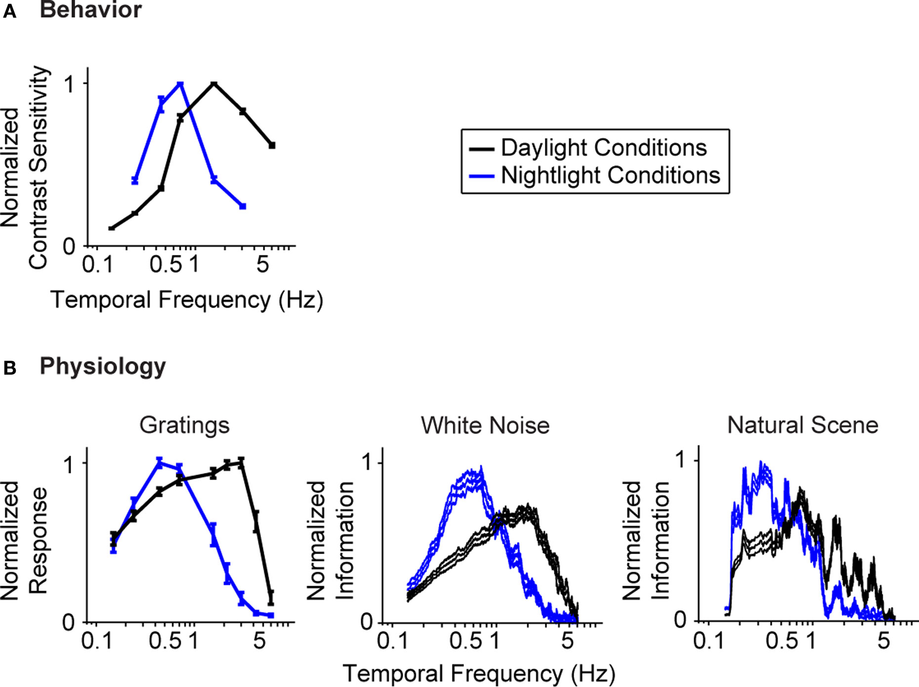
Figure 1. The visual system undergoes a shift in integration time as it shifts from daylight to nightlight (photopic to scotopic) conditions. In daylight conditions, the system favors short integration times (high temporal frequencies); in nightlight conditions, it favors long integration times (low temporal frequencies). See Materials and Methods for light intensities for the two conditions. (A) The shift, measured at the behavioral level using drifting grating stimuli. (B) The shift, measured at the ganglion cell level, using three different kinds of stimuli: drifting gratings, white noise, and natural scenes. Behavioral performance was measured as contrast sensitivity, averaged across animals, and peak-normalized (n = 5, mean ± SEM). Ganglion cell performance in (B, left) was measured as first harmonic response, averaged across cells, and peak normalized; ganglion cell performance in (B, middle and right) was measured as information, normalized for equal area (n = 20, mean ± SEM).
Figure 2
shows the proposed model for how the shift is generated. It builds on the well-established front-end circuit that shapes visual integration time (Baylor et al., 1971
; Kleinschmidt and Dowling, 1975
; reviewed in Dowling, 1987
) (Figure 2
A). The circuit contains three cell classes – photoreceptors, bipolar cells and horizontal cells – and operates, briefly, as follows: the photoreceptors send signals forward to both the bipolar and horizontal cells. The bipolar cells continue to send signals forward, while the horizontal cells send signals back onto the photoreceptors. The horizontal cell feedback shapes the photoreceptors’ integration time
1
(Baylor et al., 1971
; Kleinschmidt and Dowling, 1975
).
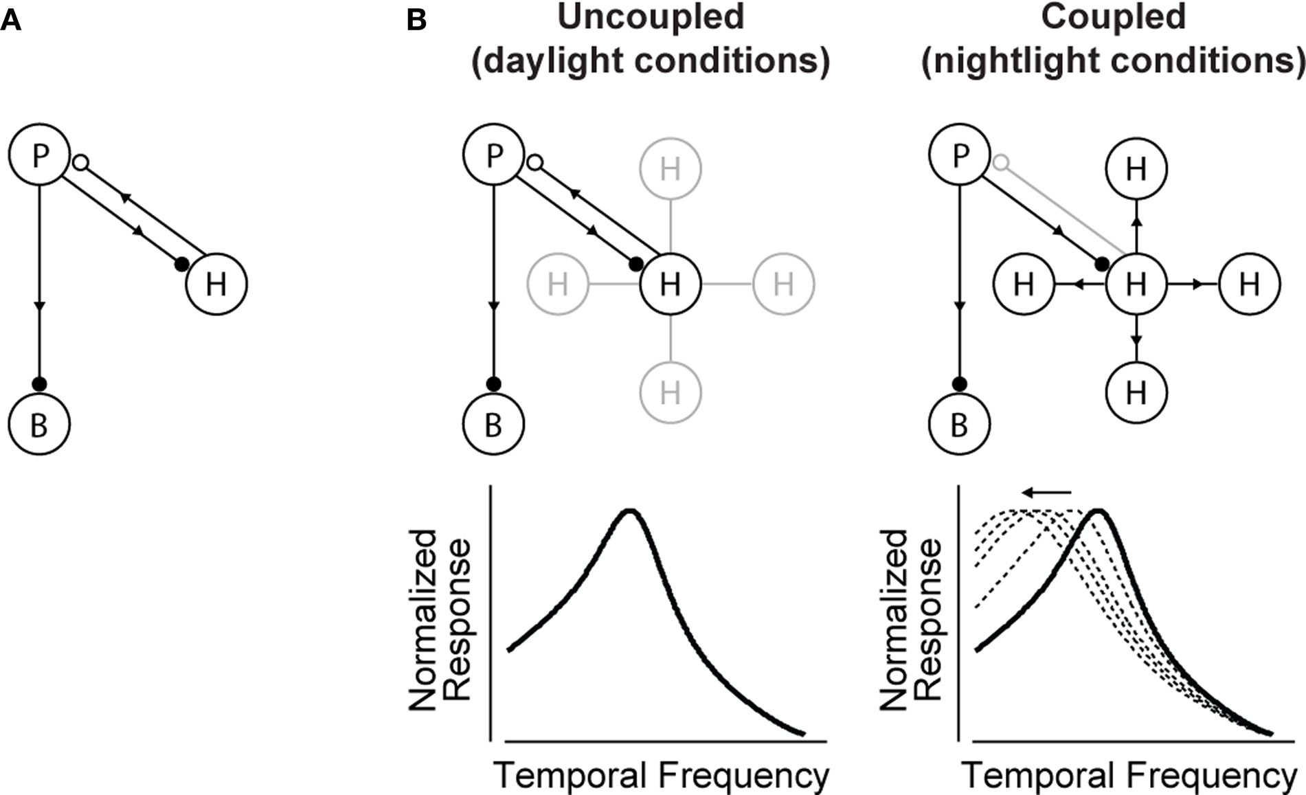
Figure 2. The circuit that controls visual integration time can be shifted from one state to another by a change in the gap junction coupling of one of its cell classes. (A) Visual integration time is shaped, in large part, by a negative feedback loop in the outer retina: photoreceptors send signals forward to both bipolar cells and horizontal cells; the horizontal cells then, in turn, provide negative feedback to the photoreceptors (Baylor et al., 1971
; Kleinschmidt and Dowling, 1975
; Dowling, 1987
). Note that the figure shows only one type of horizontal cell and a generic photoreceptor; this is consistent with our model system, the mouse retina, which has only one type of horizontal cell, and it acts on both rods and cones (Peichl and González-Soriano, 1994
; Trumpler et al., 2008
; Babai and Thoreson, 2009
). (B, left) In daylight conditions, horizontal cell feedback is strong. This cuts photoreceptor integration time short, and the system shifts to high temporal frequency responses. At night (B, right), when the system needs longer integration times, a reduction in horizontal cell feedback is needed. The opening of the gap junctions provides a mechanism for achieving this. It produces a shunting of horizontal cell current that weakens or inactivates the horizontal cells. The photoreceptor integration time then becomes longer, and the system shifts to low temporal frequency responses. The change in the gap junction coupling acts, effectively, as a knob to regulate the strength of the negative feedback. (See Appendix 2 for a formalized version of the model.)
Figure 2
B shows how a change in the gap junction coupling of the horizontal cells can modulate the circuit’s behavior – that is, how it can change it from one state to another. The scenario is the following: In daylight conditions the gap junctions close. This strengthens the signals of the horizontal cells, so they send strong feedback to the photoreceptors. Strong feedback cuts the photoreceptors’ integration time short, producing the short integration times (high temporal frequency responses) observed experimentally (Figure 2
B, left). In nightlight conditions, the gap junctions open. The opening produces a shunting of the horizontal cell current, which reduces or eliminates the horizontal cell signal. Without the feedback from the horizontal cells, there is no shortening of the photoreceptor integration time, and the system shifts to the observed long integration times (low temporal frequency responses) (Figure 2
B, right).
The strength of the model is that it derives from well-established facts – specifically, that the integration time of photoreceptors (both rods and cones) changes (becomes extended) as an animal moves from day to night conditions (Kleinschmidt and Dowling, 1975
; Daly and Normann, 1985
; Schneeweis and Schnapf, 2000
), that the strength of the horizontal cell signal changes (decreases) as the conditions move from day to night (Teranishi et al., 1983
; Yang and Wu, 1989a
), and, finally, that there is a change in the degree of horizontal cell coupling (an increase) with the change from day to night conditions (Dong and McReynolds, 1991
; Xin and Bloomfield, 1999
; Weiler et al., 2000
). Put together, these facts lead to a mechanism for shifting the circuit’s behavior. The novelty is the use of gap junction coupling as a shunting device (see Discussion) – the model makes use of the fact that coupling produces a shunt, and, therefore, has the capacity to weaken or inactivate a cell class. By casting the coupling as a shunting mechanism, the actions of the components of the circuit – the photoreceptors, the bipolar cells, the horizontal cells, and the light-dependent change in horizontal cell coupling – fall into place to explain how the system can shift from one state to another. A formalized version of the model is given in Appendix 2.
We test the proposal in Figure 3
. To do this, we used a transgenic mouse line that cannot undergo horizontal cell coupling (Hombach et al., 2004
; Shelley et al., 2006
) (Figure 3
A). These mice lack the gene for the gap junction specific to the horizontal cells, connexin 57 (Cx57), so their horizontal cells are locked into the uncoupled state. We emphasize that this particular gap junction gene is not expressed anywhere in the nervous system besides the horizontal cells (Hombach et al., 2004
); thus, the elimination of this gene produces a very specific perturbation. Figure 3
B shows the temporal integration curves from wild-type and knockout mice in the night condition, measured both at the behavioral level and at the ganglion cell level with the three stimuli used in Figure 1
. In all cases, the shift to long integration times was impaired, that is, the normal increase in amplitude at low frequencies, and the normal decrease in amplitude at high frequencies did not occur (Figure 3
B) or was significantly hindered (Figure 3
C) [p < 10−4 for the behavior, p < 10−3 for the ganglion cell responses, t-test comparing the centers of mass of the frequency response curves for the night (scotopic) condition with those for the day (photopic) condition].
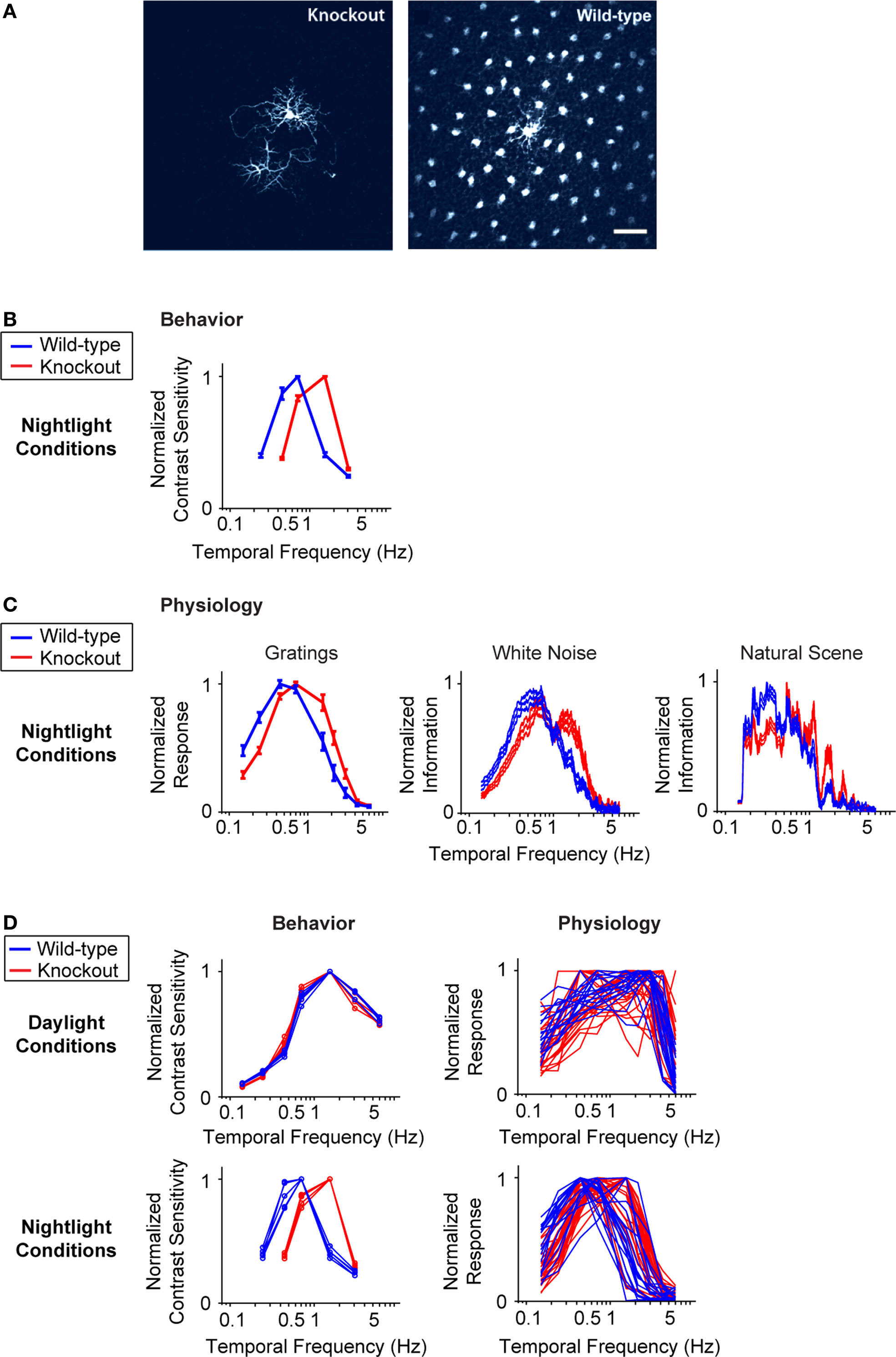
Figure 3. When horizontal cell coupling is prevented, the shift to long integration times is impaired at both the behavioral level and the ganglion cell level. (A) Horizontal cell coupling in a retina from a Cx57 knockout versus horizontal cell coupling in a retina from a wild-type sibling control. In each retina, a single horizontal cell was injected with dye, and the extent of dye spread was measured for >1 h. Consistent with the results in (Hombach et al., 2004
; Shelley et al., 2006
; Dedek et al., 2008
), coupling is abolished. Scale bar = 50 μm. (B) Behavioral performance curves measured from Cx57 knockouts and wild-type sibling controls under the night condition. The shift to long integration times (low temporal frequency responses) is significantly impaired (p < 10−4). (C) Ganglion cell performance curves measured from Cx57 knockout animals and wild-type sibling controls under the night condition. As in (B), the shift to long integration times is significantly impaired (p < 10−3). All measurements were taken as in Figure 1
; for the behavioral experiments, n = 5 wild-type mice, 5 knockout mice, and for the ganglion cell measurements, n = 20 cells from wild-type retinas, 24 cells from knockouts. (D) Left, performance for all animals shown individually. In daylight conditions, the performances of the knockouts are essentially identical to those of the wild-type animals. In night conditions, they diverge: the wild-type animals make the shift toward longer integration times, while the knockouts do not. Right, performance for all ganglion cells. Similar to plots on the left, the performances of the ganglion cells from the knockout and wild-type animals are the same in daytime conditions but diverge at night: the ganglion cells from the wild-type animals undergo the shift toward longer integration times, while those from the knockout are left behind.
The robustness of the results is demonstrated in Figure 3
D. Using data that allow a direct comparison to be made between behavioral and ganglion cell results, specifically, where the results were obtained using the same stimuli – the drifting sine wave gratings – we show the complete set of individual responses. The left side of Figure 3
D shows the behavioral performance for all animals under day and night conditions, and the right side shows the performance for all ganglion cells under day and night conditions. As shown in the figure, by day, the performance of the knockout closely matches that of the wild-type, but at night, the two performances diverge. At night, the wild-type makes the expected shift toward longer integration times, but the knockout – which lacks horizontal cell coupling – does not.
The nervous system faces a shifting problem. It has to shift its mode of operation from one state to another as it faces new demands (i.e., it has to shift its attention, its contrast sensitivity, its temporal integration time, etc.). How it achieves this isn’t clear. Here we examined a case where it was possible to obtain an answer, and the answer was intriguingly simple: the system produced the shift by changing the gap junction coupling of one of its cell classes. The coupling acted as a way to inactivate the cell class, and, by doing so, change the system’s behavior.
The findings are both surprising and exciting: surprising, because a seemingly complicated problem was solved with a simple mechanism, and exciting, because the mechanism is present not just in the retina, but throughout the brain, suggesting it might generalize to other network shifts. To be specific, gap junction coupled networks are present in visual cortex, motor cortex, frontal cortex, hippocampus, cerebellum, hypothalamus, and striatum, among many other places (Galarreta and Hestrin, 1999
, 2001
; Bennett and Zukin, 2004
).
Furthermore, a regulator is also in place. In the retina, the regulator is a neuromodulator, dopamine: Light triggers the release of dopamine, which closes gap junctions via second messengers (McMahon et al., 1989
; Dong and McReynolds, 1991
; Weiler et al., 2000
). Dopamine, as well as noradrenaline and histamine, have been found to open and close gap junctions in several of these brain areas (Cepeda et al., 1989
; Yang and Hatton, 2002
; Onn et al., 2008
; Zsiros and Maccaferri, 2008
).
The possibility for generalization to other networks is substantial and straightforward to see:
(1) While the results in this paper show the mechanism in non-spiking neurons, it readily applies to spiking cells as well and thus to networks in the brain. This is because the mechanism involves only basic biophysics – a change in cells’ input resistance. Briefly, if a cell class is coupled by gap junctions, it has the potential to have its input resistance turned up and down. When the junctions are closed, the input resistance of the cells is high. This makes the cells more responsive to incoming signals and allows them to send strong signals out. When the junctions are opened, the input resistance drops. This makes the cells less responsive to incoming signals and allows them to send out only weak signals. In the case of spiking neurons, the signals can become so weak that the probability of firing can be reduced essentially to 0; i.e., the cells can be effectively turned off.
(2) The mechanism has the potential to affect many types of network operations. While the one presented in this paper was a negative feedback loop – the gap junction coupling provided a way to turn the feedback on or off (or up or down) – one can readily imagine many other operations that could be altered by turning the activity of a pivotal cell class in a network on or off, such as alterations in feedforward signaling, lateral signaling, recurrent signaling (e.g., the stabilization of attractors), to name a few.
(3) The timescale over which the mechanism operates, that is, the timescale over which the change in coupling occurs – a scale of seconds (McMahon et al., 1989
; McMahon and Mattson, 1996
) – is consistent with many state changes, such as changes in arousal, changes in attentional set, shifts in decision-making strategies, e.g., shifts in the weighting of priors, shifts to speed versus accuracy (Standage and Paré, 2009
), allowing it to mediate many behavioral processes.
(4) Since the cellular machinery for regulation of gap junction conductances is in place, the mechanism can evolve via a change in a single gene, a gene for a gap junction protein. This makes it an easy gain from an evolutionary standpoint. A powerful selective advantage – the ability to shift a network from one state to another – could be rapidly acquired, and, in addition, acquired independently in multiple networks. (For a review of gap junction proteins, see Bennett and Zukin, 2004
.)
Figure 4
emphasizes this latter point, that this gap junction coupling mechanism offers a single gene solution to a seemingly complicated set of problems, network state changes. To address this, we used, again, the horizontal cells, as an example. Specifically, we took the behavioral results from the wild-type and Cx57 knockout animals and imposed them on a predator-detection scenario. We filmed an approaching predator, restricting the movies to the temporal frequencies available to each genotype, as indicated in Figure 3
D left. The results are shown in Figure 4
. In day conditions the movies for the two genotypes are essentially the same; the predator can be seen when it is moving, i.e., when the movie is dominated by high temporal frequencies, and when it is still, i.e., when the movie is dominated by low temporal frequencies. In contrast, in night conditions, the movies diverge. In the movie filtered through the frequencies visible to the wild-type animal, the predator remains visible even when it is still; this is consistent with the wild-type’s ability to shift to low temporal frequencies. In the movie filtered though the frequencies visible to the knockout, the predator disappears. Only a ghost is present (see Supplementary Material for the complete movies). The wild-type’s maintenance of visual contact with the predator gives it an obvious selective advantage.
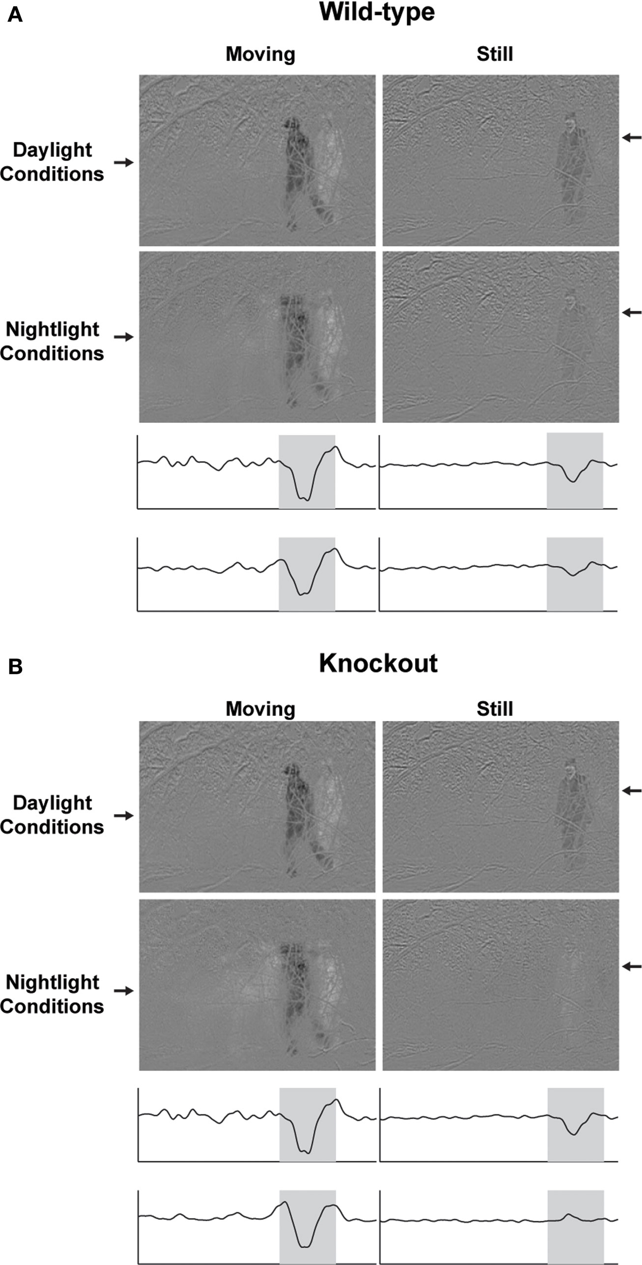
Figure 4. The selective disadvantage of a Cx57 gene loss. (A) Movie of an approaching predator, filtered through the frequencies available to the wild-type animal, as provided by Figure 3
D left. In day conditions, the predator can be seen both when it is moving (when the movie is dominated by high temporal frequencies), and when it is still (when the movie is dominated by low temporal frequencies). In night conditions, the signal is weaker, but the predator can still be seen both when moving or still. The visibility in the still condition is possible because of the shift to low temporal frequencies that occurs in the dark. The traces below the figures provide the intensity of each pixel in a horizontal slice through the image; the location of the slice is indicated by the arrow. (B) Same movie, filtered through the frequencies available to the knockout animal. In night conditions, the predator vanishes, see trace below figures. The wild-type’s continued visual detection of the predator gives it an obvious selective advantage. (For the frequencies available to each genotype, see Figure 3
D left: specifically, the range of frequencies seen by the knockout at night (red curves in 3D bottom left) is a subset of the range seen by the wild-type (blue curves); the lack of low frequency sensitivity in the knockout (below ∼0.3 Hz) causes the predator, when it is still, to disappear. Note that the temporal filtering was applied to the entire movie; only a representative frame from each filtered version is shown here. For the complete filtered versions, see Supplementary Material).
Estimating the Extent to Which Input Resistance can be Reduced by Coupling
As discussed above, changes in coupling can act as a dial to turn the input resistance of a cell up or down. We can estimate the range of the dial as follows: The standard experimental measure of coupling is the length constant (Xin and Bloomfield, 1999
; Shelley et al., 2006
). Xin and Bloomfield measured the length constant of horizontal cells under several scotopic and photopic light levels and found the maximal difference to be a factor of ∼3. The maximal difference occurred when the scotopic light level was 1–1.5 log units above rod threshold and the photopic light level was >3 log units above rod threshold, levels that we matched for this paper. Since, for 2-D coupling (Lamb, 1976
), input resistance is inversely proportional to the square of the length constant (detailed in Materials and Methods and Appendix 2), the input resistance of the horizontal cells at the scotopic light level is estimated to be about a factor of 9 less than that at the photopic light level.
In the general case, as with horizontal cells, the extent to which gap junction coupling can shunt a cell is the ratio of the total conductances of the gap junctions that can be modulated, to the cell’s baseline (“leak”) conductances. Many factors – including the cell’s geometry and the complement and distribution of channels and gap junctions – combine to determine this ratio. The example of horizontal cells shows that this can be as much as an order of magnitude.
Linking a Behavior to a Neural Mechanism
Following a behavioral change down to the mechanism that underlies it is often not possible experimentally. It was possible here because of a confluence of factors: the relevant network could be identified and its component cell classes are known (as shown in Figures 1 and 2
), and the protein around which the mechanism revolves, the particular gap junction protein, Cx57, is present only in one cell class (the horizontal cells) and not elsewhere in the brain (Hombach et al., 2004
), allowing the circuit to be selectively disrupted. The significance of the latter is that it allowed a direct connection to be made between the disruption in the circuit and the disruption in the behavior, since no other circuits were perturbed.
Potential Alternative Models for the Shift Toward Low Temporal Frequencies
As an animal moves from a light-adapted to a dark-adapted state, several changes occur in the retina other than the change in horizontal cell coupling via the Cx57 gap junctions. How can we be sure that our result – the shift toward low temporal frequencies – is not produced by these other changes? Here we systematically go through them.
The most well known change is the shift from cone to rod photoreceptors. This can’t account for our results, because the knockout undergoes the same cone-to-rod shift, and it doesn’t undergo the shift to low frequencies (Figure 3
). In addition, it’s well known that the cone-to-rod shift affects high frequencies, not low. We show this in Appendix 1, Figure 5
, specifically for our species, the mouse. As shown in the figure, the frequency response curves for the rod and cone are both flat below 0.5 Hz, meaning there is no frequency-dependent change in this region. In contrast, our results show a selective boost at frequencies below 0.5 Hz; that is, the system shifts to favor low frequencies. The shift from cones to rods can’t account for this.
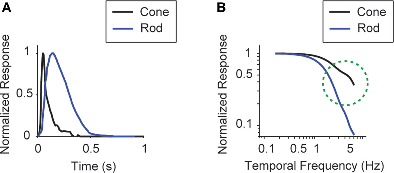
Figure 5. The frequency response difference between the rods and cones lies in the high frequencies, not the low. (A) Impulse responses of the two photoreceptors, reproduced from Nikonov et al. (2006)
for cone and Luo and Yau (2005)
for rod. (B) Frequency responses of the two photoreceptors, generated by Fourier transforming the impulse responses.
Another change that occurs during dark adaptation is rod–cone coupling (see Ribelayga et al., 2008
, for rod–cone coupling as a result of circadian rhythms; also Yang and Wu, 1989b
; Wang and Mangel, 1996
; Trumpler et al., 2008
). Rod–cone coupling, though, is mediated by gap junctions formed by Cx36, Cx35, and Cx34.7 (reviewed in Li et al. (2009)
), not Cx57 (Janssen-Bienhold et al., 2009
). Cx57 is not present in rods and cones (Hombach et al., 2004
; Janssen-Bienhold et al., 2009
) and thus the knockout is not perturbing these couplings.
Similarly, gap junction coupling in the inner retina likely plays a role in dark adaptation, since the AII amacrine cells of the rod pathway are coupled by gap junctions (Bloomfield et al., 1997
). However, Cx57 is not a gap junction in these cells (Janssen-Bienhold et al., 2009
), so changes in inner retinal coupling can not account for our results.
Recent reports have indicated that some gap junctions act as hemichannels (Kamermans et al., 2001
; Shields et al., 2007
). If Cx57 acted in this fashion, it could provide for ephaptic transmission of a feedback signal. However, the possibility that Cx57 is a hemichannel has been examined at the ultrastructural level, and ruled out (Janssen-Bienhold et al., 2009
). Furthermore, feedback to photoreceptors has been shown to be intact in the Cx57 knockout by two groups (Shelley et al., 2006
; Dedek et al., 2008
).
Finally, a standard concern with most or all knockout experiments is that knocking out a gene could lead to secondary developmental effects. While we can’t completely rule this out, there is no evidence for altered development in the Cx57 knockout: retinal anatomy appears unperturbed (Hombach et al., 2004
; Shelley et al., 2006
), temporal tuning by day, as measured at the ganglion cell and behavioral level, remains intact, i.e., is the same as in wild-type (Figure 3
D), and spatial processing, also measured at the ganglion cell and behavioral level, remains intact as well (Dedek et al., 2008
). While compensatory effects are possible, the likelihood that they would lead to such close matches along all these axes is very low.
Thus, while cone-to-rod shifts, photoreceptor coupling, and other factors contribute to dark adaptation, they can’t account for the results presented here, and the probability that the results could be accounted for by developmental effects, as mentioned above, is very low.
One issue that we can’t completely rule out, though, is the following: even though horizontal cell feedback to photoreceptors is known to be present and can account for our results, we can’t completely rule out the possibility that the shunting of horizontal cell current causes the shift in tuning through some other action. For example, if horizontal cells were to act as a mediator between multiple circuits with different kinetics (e.g., different photoreceptor readout circuits), then the shunting of the horizontal cell current could shift tuning by causing a switch from one circuit to another. But note that any alternative model must be consistent with the known constraints: (a) the difference between wild-type and knockout is present under scotopic conditions (Figure 3
), where all responses are rod-driven, (b) the tuning shift involves low frequencies, (c) the mouse retina has only one kind of horizontal cell, and it serves both kinds of photoreceptors, and (d) connexin-57 is only involved in horizontal cell-to-horizontal cell coupling. We chose the horizontal cell feedback model shown in Figure 2
because it is a parsimonious model that satisfies these constraints and is consistent with current known actions of horizontal cells.
We conclude by mentioning that in one species (the rabbit), when light levels are much lower, more than an order of magnitude below the scotopic level used in this study, gap junctions close (Xin and Bloomfield, 1999
) with no corresponding reversal of the shift in integration times (Nakatani et al., 1991
). This suggests that in this extreme range, other mechanisms must take over, mechanisms likely intrinsic to the photoreceptors, as described in Tamura et al. (1989)
.
Relation of Cx57 to Spatial Processing In the Dark- and Light-Adapted Conditions
Horizontal cells provide negative feedback to photoreceptors (Werblin and Dowling, 1969
) and antagonistic feedforward to bipolar cells (Yang and Wu, 1991
), and it has long been thought that they contribute to the receptive field surround. One might expect, therefore, that eliminating coupling in these cells would alter spatial processing as well as temporal processing as the retina shifts from day to night vision. A previous study, though, shows that spatial tuning remains normal in the Cx57 knockout (Dedek et al., 2008
). The likely basis for this is the fact that the surround is generated by circuits in more than one layer – specifically, by amacrine cell circuits in the inner retina, as well as by horizontal cells in the outer retina (Cook and McReynolds, 1998
; Taylor, 1999
; Roska et al., 2000
; Flores-Herr et al., 2001
; McMahon et al., 2004
; Sinclair et al., 2004
). As mentioned in Dedek et al. (2008)
, the lack of a change in spatial tuning in the knockout implies that inner retinal mechanisms dominate for the problem of adjusting spatial tuning to different light-adaptation levels.
Coupling as a Mechanism to Produce Synchrony
We conclude by mentioning that gap junction coupling has also been proposed as a mechanism to create synchronous firing among neurons, e.g., for creating oscillations (for review, see Bennett and Zukin, 2004
). The idea presented in this paper – that changes in coupling serve as a way to inactivate a cell class or reduce its impact – is not mutually exclusive with this proposal. This is because the effect of coupling depends on the state of the cell. As mentioned above, when a cell becomes coupled to other cells, its input resistance drops. For spiking neurons, this means the probability of reaching threshold and firing is reduced. If, however, the cell receives strong enough input to allow it to cross threshold, its firing can produce synchronous spikes in coupled cells. Thus, gap junction coupling can potentially mediate more than one network operation.
Animals
Generation of the Cx57-deficient mouse line was previously reported (Hombach et al., 2004
). Briefly, part of the coding region of the Cx57 gene was deleted and replaced with the lacZ reporter gene (Hombach et al., 2004
). Cx57-deficient mice (Cx57lacZ/lacZ) and wild-type (littermate) controls aged 2–4 months were used for all experiments. After each behavioral test or recording, the genotype of the retina was confirmed with staining for β-galactosidase activity and PCR as described (Hombach et al., 2004
). All experiments were conducted in accordance with the institutional guidelines for animal welfare.
The Degree of Horizontal Cell Coupling and Light Intensity
Light intensities (photopic and scotopic) were chosen to span the range where changes in horizontal cell coupling are at, or are close to, their largest. Xin and Bloomfield (1999)
showed that coupling reaches its maximum between 1 and 1.5 log units above rod threshold and its minimum at or above rod saturation (estimated at 3 log units above rod threshold). For the behavior experiments, scotopic intensity was 1.4 × 10⁻⁴ cd/m2, which is between 0.9 and 2.1 log units above rod threshold, with mouse rod threshold estimated at 1 × 10⁻⁶ to 1.8 × 10⁻⁵ cd/m2 (GUmino et al., 2008
; .T. Prusky, Personal communication). Photopic intensity, 142 cd/m2, was more than 3 log units above rod saturation (Xin and Bloomfield, 1999
). The light source was Dell, 2007FPb, Phoenix, AZ, USA; neutral density filters were used to attenuate the monitor’s output to the desired photopic and scotopic levels.
For the electrophysiology experiments, which were carried out with a different light source (Sony, Multiscan CPD-15SX1, New York, NY, USA), the intensities were, for the scotopic, 4 × 10⁻⁴ cd/m2, which is between 1.3 and 2.6 log units above rod threshold, and, for the photopic, 23 cd/m2, which is still >3 log units above rod saturation. As above, neutral density filters were used to attenuate the monitor’s output to the desired photopic and scotopic levels.
The Relation of Horizontal Cell Input Resistance to Coupling for Scotopic Versus Photopic Conditions and for Wild-Type Versus Knockout Animals
As mentioned in the Discussion, the standard experimental measure of horizontal cell coupling is the length constant (Xin and Bloomfield, 1999
; Shelley et al., 2006
). Xin and Bloomfield measured length constants physiologically in the rabbit (via the dependence of the voltage response on distance from a light stimulus) under different scotopic and photopic conditions and found the maximal scotopic-to-photopic ratio to be ∼3. (As indicated in the previous section, the conditions used in this paper were matched to those that produce the maximal ratio.) Given this length constant ratio and the relations below, we can find the quantity we need, the input resistance ratio due to gap junction coupling. As given in Xin and Bloomfield (1999)
,
where λ is the length constant, Rm is the membrane resistance, and Rs is the junctional resistance (also referred to as the sheet resistance). Rearranging in terms of Rs gives

For a 2-D cable and a point source, the input resistance, Z, is proportional to Rs. This follows from Eq. 2 of Lamb (1976)
(see Appendix 2 Eqs 14–19 for details). Thus, it follows from Eq. 2 that

This indicates that a 3-fold greater value of λ, as was measured by Xin and Bloomfield, corresponds to a 9-fold smaller value of Z, assuming that Rm remains the same in the scotopic and photopic conditions. Bloomfield notes that Rm may actually be higher in the photopic, indicating that a factor of 9 may be an underestimate.
The same analysis can be used to determine the input resistance ratio for the knockout and wild-type mouse using the measurements of Shelley et al. (2006)
, which were taken in these animals. These measurements, however, were taken only at one light level, and thus can provide only a lower bound on the ratio. Shelley et al. report a 2.3-fold greater value for λ in wild-type as compared to knockout, which, following Eq. 3, corresponds to a 2.32 = 5.29-fold lower value for Z. It should be noted that Rm, as measured in isolated horizontal cells, is 27% lower in the knockout than the wild-type. When this is taken into account in Eq. 3, the wild-type-to-knockout ratio for Z is (1 − 0.27)/(1/2.32) = 3.86. We emphasize again that this is a lower bound on the input resistance ratio, since, as mentioned above, Shelley et al. measured length constants in knockout and wild-type only at a single light level.
Note that the 27% decrease in Rm has an additional implication: the observed change in temporal tuning that results from the change in coupling constitutes a lower bound, as the decrease in Rm would have the effect of reducing the difference between knockout and wild-type.
Behavioral Testing Using a Virtual Optokinetic System
Behavioral responses were measured using the Prusky/Douglas virtual optokinetic system (Prusky et al., 2004
; Douglas et al., 2005
). Briefly, the freely moving animal was placed in a virtual reality chamber. A video camera, situated above the animal, provided live video feedback of the testing arena. A pattern was projected onto the walls of the chamber in a manner that produced a drifting sine wave grating of fixed spatial frequency when viewed from the animal’s position (0.128 cycles/degree, following the stimulus protocol of Umino et al., 2008
). A drifting grating of a pre-selected temporal frequency at 100% contrast appeared, and the mouse was assessed for tracking behavior, as in Prusky et al. (2004)
. Grating contrast was systematically reduced until no tracking response was observed. The reciprocal of this threshold contrast was taken as the contrast sensitivity.
Stimulating and Recording Ganglion Cell Responses
Three stimuli were used: drifting sine wave gratings, a binary random checkerboard (white noise), and a spatially uniform stimulus with natural temporal statistics (natural scene). The sine wave gratings were presented at eight temporal frequencies, ranging from 0.15 to 6 Hz, all with a spatial frequency of 0.039 cycles/degree. This spatial frequency was lower than the one used in the behavioral experiments, to ensure robust responses at the scotopic intensity. Each temporal frequency was presented for 2 min. The white noise stimulus was a random checkerboard at a contrast of 1, in which the intensity of each square (9° × 9° in mouse) was either white or black, randomly chosen every 0.067 s (large checkers were chosen to ensure stimulation of the large ganglion cell receptive fields at scotopic intensities, as indicated in Dedek et al., 2008
). The natural scene stimulus was a spatially uniform movie whose intensities were taken from a time series of natural intensities (van Hateren, 1997
), resampled for presentation at a 0.100-s frame period. This movie was 2 min long and presented 10 times, interleaved with a 2-s gray (mean intensity) screen. Measurements always started at the scotopic intensity. After all three stimuli were presented, the light intensity was increased. After 20 min of adaptation to the photopic intensity, the stimuli were presented as above.
Extracellular recordings made from central retina using a multi-electrode array, as described previously (Nirenberg et al., 2001
; Sinclair et al., 2004
). Retina pieces were approximately 1.5–2 mm across, which corresponds to 4.5–6 horizontal cell length constants under scotopic conditions and 15–20 under photopic (as indicated above, there is an estimated factor of 3 difference in length constant between the scotopic and photopic conditions used here, with the photopic condition taken from Shelley et al. (2006)
Figure 7
B, which gives a wild-type light-adapted length constant). Spike trains were recorded and sorted into units (cells) using a Plexon Instruments Multichannel Neuronal Acquisition Processor (Dallas, TX, USA), as described previously (Nirenberg et al., 2001
).
Only ON ganglion cells were used, since the optomotor response in rodents is driven exclusively by the ON pathway (Dann and Buhl, 1987
; Giolli et al., 2005
). With respect to cell selection, only cells with readily detectable (by eye) spike triggered averages (STAs) were included in the data set; this corresponds to cells whose STA in the center checker of the receptive field was approximately 1.5 times above background.
Data Analysis
Temporal tuning curves were created from ganglion cell responses to drifting sine wave gratings using standard methods (Enroth-Cugell and Robson, 1966
; Purpura et al., 1990
; Croner and Kaplan, 1995
). Briefly, for each grating, the first harmonic of the cell’s response, R(f), was calculated as follows:
where f is the temporal frequency of the drifting sine wave grating (cycles/s), L is the duration of the stimulus (s), which was always an integer multiple of 1/f, and tj is the time of the jth spike of the cell’s response to the given grating. For averaging across cells, responses were weighted by the reciprocal of the peak sensitivity, so that each cell’s tuning curve contributed approximately equally to the average, independent of its absolute sensitivity.
Mutual information was estimated between the input and responses (for the white noise, the input was the stimulus intensity of the checkerboard square that produced the largest response for a given cell; for the natural scene, the input was the full-field intensity). Information was estimated at each frequency using the coherence rate, following van Hateren and Snippe (2001)
:

where γ(f) is the coherence between stimulus and response at temporal frequency f. Coherence was estimated using the multi-taper method [Chronux library for Matlab (Mitra and Bokil, 2007
), available at http://chronux.org
, using effective bandwidths of 0.27 Hz (white noise) and 0.33 Hz (natural scene). For averaging across cells, information curves were weighted by the reciprocal of their areas, so that each cell’s information curve contributed approximately equally to the average. Note that the above estimation of information is only rigorously correct for a Gaussian linear channel, and is necessarily an underestimate of the true information. However, our focus is not on the amount of information per se, but on its frequency-dependence.
Filtered Predator Movies
The “predator” movie, taken with a handheld digital camera (Casio, Exilim EX-Z750, Dover, NJ, USA), was filmed at 33 frames/s. The complete movie was filtered for each genotype, according to the behavioral data in Figure3
D left: 0.1–6 Hz for the wild-type photopic, the same for knockout photopic, 0.16–3.2 Hz for wild-type scotopic, and 0.38–3.13 Hz for knockout scotopic. Representative frames from each filtered version are shown in Figure 4
; the complete filtered versions are shown in Supplementary Material.
The Frequency Response Difference Between the Rods and Cones Lies in the High Frequencies, not the Low
The shift to low temporal frequencies cannot be accounted for by the shift from cones to rods, as the cone-to-rod shift affects the high frequencies, not the low; see cone and rod impulse responses in Luo and Yau (2005)
, Nikonov et al. (2006)
. Here we show this explicitly in the model system we are using, the mouse. Figure 5
A shows the impulse responses of the two photoreceptors, and Figure 5
B shows the frequency responses, the latter generated by the Fourier transformation of the impulse responses. As shown in the figure, the frequency response difference lies in the high frequencies.
Formal Treatment of the Model In Figure 2 : The Effect of Gap Junction Coupling on Horizontal Cell Feedback to the Photoreceptor
Section A formalizes the model of the photoreceptor–horizontal cell circuit to show how changing the strength of the horizontal cell feedback shapes the photoreceptor’s temporal tuning, and, ultimately, the ganglion cell’s temporal tuning. Section B then shows how a change in gap junction coupling modulates the strength of the horizontal cell feedback. Section C describes how these considerations apply to spatial configurations of the stimulus, and Section D briefly discusses how these considerations apply to other network geometries.
Section A
We start by briefly reiterating the model shown in Figure 2
. As mentioned in the main text, it builds on the well-known negative feedback between the horizontal cell and the photoreceptor, whereby the horizontal cell sends a signal to the photoreceptor that shortens the latter’s integration time (Baylor et al., 1971
; Kleinschmidt and Dowling, 1975
; see also Smith, 1995
).
To understand how the photoreceptor is able to shift its integration time from short to long as the retina is shifted from a light-adapted to a dark-adapted state, we proposed the following: In the light-adapted condition, the gap junctions of the horizontal cells close. This makes the horizontal cell feedback signal strong and keeps the photoreceptor integration time short. In the dark, the gap junctions open. This causes a shunting of horizontal cell current, which reduces horizontal cell feedback and shifts the photoreceptors to long integration times.
The proposal is based on three established facts – that the integration time of photoreceptors increases as the retina moves from light-adapted to dark-adapted conditions (Kleinschmidt and Dowling, 1975
; Daly and Normann, 1985
; Schnapf et al., 1990
), that the strength of the horizontal cell feedback signal decreases as the retina moves from the light-adapted to the dark-adapted condition (Teranishi et al., 1983
; Yang and Wu, 1989a
) and that the degree of horizontal cell coupling increases as the retina moves from the light adapted to the dark-adapted condition (Dong and McReynolds, 1991
; Xin and Bloomfield, 1999
; Weiler et al., 2000
). Taken together, these facts led to a proposal for how the circuit shifts its behavior. The novelty was the view of gap junction coupling as a shunting device, that is, a mechanism that can turn up or down the activity of a cell class, in this case, the horizontal cells. With this view, the three facts can account for the shift from one state to another.
In the main text, we proposed this schematically. Here we formalize it and use the formalized model to determine the feedback strength required to produce the observed state change.
We start with the well-known data of Schneeweis and Schnapf (2000)
. The data are measurements of photoreceptor responses across a range of light-adaptation levels and show the shift in integration time that occurs as the retina moves from the dark-adapted state to states of increasing levels of light-adaptation. We use the model to determine the change in feedback strength needed to produce the changes in photoreceptor integration time in Schneeweis and Schnapf (2000) and, ultimately, to produce the changes in ganglion cell integration time shown in this paper. (In Section B we show that the changes in feedback strength can be accounted for by the differences in horizontal cell coupling that occur in the dark- and light-adapted states.)
With these goals in mind, we use a linear systems approach. We do this for simplicity and generality, and because it allows us to focus on the essential features that lead to the shifts.
To construct the linear model, we denote the transfer function between light and the photoreceptor response in the absence of the feedback by  , the feedback transfer function (photoreceptor output to horizontal cell, and back to photoreceptor) by
  , and the strength of the feedback by g. With this setup, the photoreceptor’s output,
  is given by the standard feedback formula (Oppenheim et al., 1997
)
is given by the standard feedback formula (Oppenheim et al., 1997
)
, the feedback transfer function (photoreceptor output to horizontal cell, and back to photoreceptor) by , and the strength of the feedback by g. With this setup, the photoreceptor’s output, is given by the standard feedback formula (Oppenheim et al., 1997
)
To assign physiological values to the quantities in Eq. 6, we use, as mentioned above, the measurements of Schneeweis and Schnapf (2000)
, who present photoreceptor responses in the dark-adapted state (i.e., the no-feedback or essentially-no-feedback state, g = 0) through several light-adapted states (i.e., various levels of feedback up to g = 1) (Figure 6
).
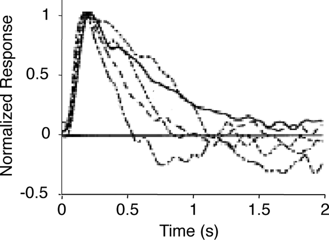
Figure 6. Measured photoreceptor responses at increasing levels of light adaptation. Photoreceptor (macaque rod) responses under dark-adapted conditions (solid curve) and at increasing levels of light adaptation (dashed curves). The dark-adapted curve corresponds to the no-feedback or essentially-no-feedback condition; the light-adapted curves correspond to increasing levels of feedback. Adapted from Schneeweis and Schnapf (2000)
Noise and light adaptation in rods of the macaque monkey. Visual Neuroscience 17, pp. 659–666, with permission of the publisher, Cambridge University Press. Curves are peak-normalized and inverted so that light responses are plotted up.
We determine the photoreceptor transformation P directly from Schneeweis and Schnapf’s dark-adapted data, since when g = 0, P = L (see Eq. 6). Specifically, we use their fit for P(t), which is a phenomenological fit, given by:
 , where
and A = 3999, B = 1.68, τ1 = 0.063 s, τ2 = 0.646 s, τ3 = 0.200 s, n = 3, and m = 4. The corresponding transfer function  is then determined from the impulse response P(t) by Fourier transformation. Both P(t) and
  are shown in Figure 7
A.
are shown in Figure 7
A.
is then determined from the impulse response P(t) by Fourier transformation. Both P(t) and are shown in Figure 7
A.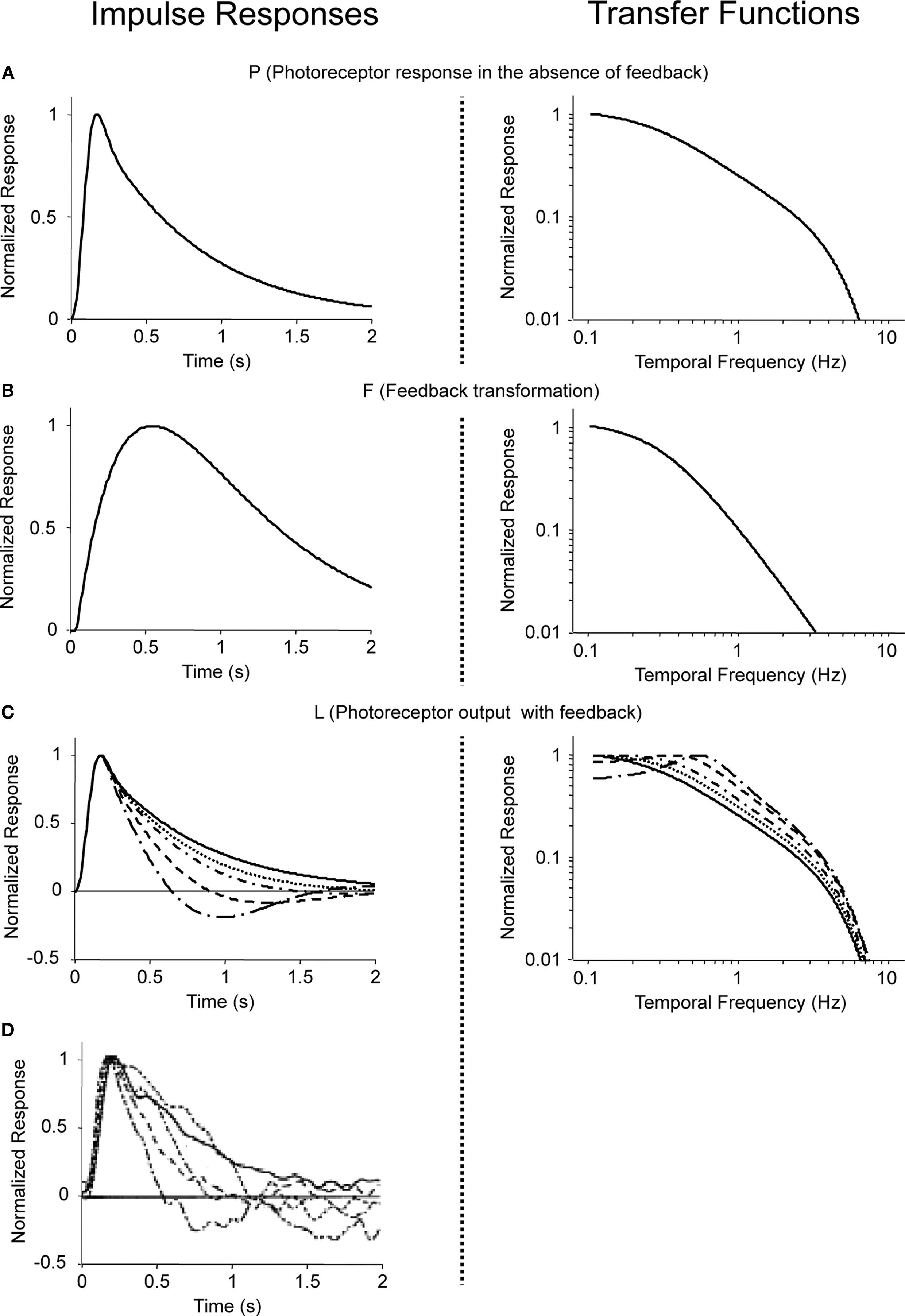
Figure 7. Modeled photoreceptor responses at increasing levels of light adaptation. Impulse responses (left) and transfer functions (right) for the components of a simple feedback model of photoreceptor responses at increasing levels of light adaptation. (A) P, the response of the photoreceptor in the absence of feedback, corresponding to the dark-adapted state. (B) The feedback transformation F. (C) The resulting photoreceptor output, L (Eq. 6). The g = 0-curve (solid) is the same as (A); the dashed curves correspond to g = 0.1, 0.2, 0.5, and 1. (D) The photoreceptor responses reported by Schneeweis and Schnapf (2000)
, as in Figure 6
. All curves are shown peak-normalized; transfer functions are plotted as a function of frequency, f = ω/2π.
We then determine the feedback transformation F from the light-adapted measurements of Schneeweis and Schnapf. Since F was not measured directly, we proceed as follows. As mentioned above, F is the net result of two synapses in series: photoreceptor to horizontal cell, and horizontal cell back to photoreceptor. For simplicity, we use the same impulse response f(t) for each synapse, and we use a difference of exponentials, a standard synaptic impulse response (Destexhe et al., 1995
) for its functional form:

Since the two synapses act in series, the feedback transfer function  is proportional to the product of the transfer functions at each synapse. We also include an overall scale factor F0 in
  , so that we can pin the modeled response at g = 1 to the measured response at the highest level of light adaptation. Since we use the same transfer function
  for the two synaptic components of F, the transfer function of the feedback transformation is given by
is proportional to the product of the transfer functions at each synapse. We also include an overall scale factor F0 in , so that we can pin the modeled response at g = 1 to the measured response at the highest level of light adaptation. Since we use the same transfer function for the two synaptic components of F, the transfer function of the feedback transformation is given by
The parameters (τa = 0.5 s, τb = 0.01 s, δ = 0.01 s, and F0 = 10) are chosen so that for a maximal feedback strength of g = 1, the photoreceptor output L given by Eq. 6 matches the most light-adapted response obtained by Schneeweis and Schnapf. The feedback impulse response F(t) is the inverse Fourier transform of  ; both are shown in Figure 7
B. As seen in Figure 7
C, without changing this feedback transformation – just changing its strength g – the feedback model accounts for Schneeweis and Schnapf’s responses at intermediate light levels.
; both are shown in Figure 7
B. As seen in Figure 7
C, without changing this feedback transformation – just changing its strength g – the feedback model accounts for Schneeweis and Schnapf’s responses at intermediate light levels.
; both are shown in Figure 7
B. As seen in Figure 7
C, without changing this feedback transformation – just changing its strength g – the feedback model accounts for Schneeweis and Schnapf’s responses at intermediate light levels.To summarize, then, the modeled photoreceptor responses (Figure 7
C) closely match the observed photoreceptor responses of Schneeweis and Schnapf (Figure 6
) (also reproduced in Figure 7
D for the reader’s convenience). This enables us to obtain an estimate of the horizontal cell feedback strength needed to produce the range of changes in photoreceptor tuning. As shown in the figure, an approximate 10-fold change is needed: since g = 0 and 0.1 give nearly identical responses, we take g = 0.1 as the lower end of the range.
We now relate the photoreceptor output to the ganglion cell output. Specifically, we take into account the transformations that occur in the second processing layer of the retina (the inner plexiform layer). While these transformations have many details (Werblin and Dowling, 1969
; Victor, 1987
; Sakai and Naka, 1988
), the common denominator is that signals become more transient, i.e., high-pass filtering occurs. We represent this with a standard RC filter in feedback configuration,

choosing the parameter values (kI = 4 and τI = 6 s) to match the dark-adapted ganglion cell response, as in Figure 3
C (wild-type). Thus, the ganglion cell response is determined by the output of the photoreceptor–horizontal cell feedback circuit (Eq. 6), followed by the schematic inner plexiform layer filter (Eq. 10):
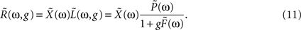
Figure 8
shows the results. Figure 8
A recapitulates the photoreceptor output from Figure 7
C, and Figure 8
B shows the corresponding ganglion cell output after applying Eq. 11. (Figure 8
C shows the same result on a semilog plot, to be consistent with the main text.) As shown in Figure 8
C, as horizontal cell feedback strength decreases, the temporal tuning of the ganglion cell response shifts to lower frequencies. The shift in the peak frequency is approximately 3-fold, from 0.6 to 0.2 Hz, and can be accounted for by a factor of 10 reduction in horizontal cell feedback strength. Since the shift we observe in Figure 3
C is a subset of this, a 10-fold change in feedback strength more than suffices to account for the shift in tuning we observe at the ganglion cell output.
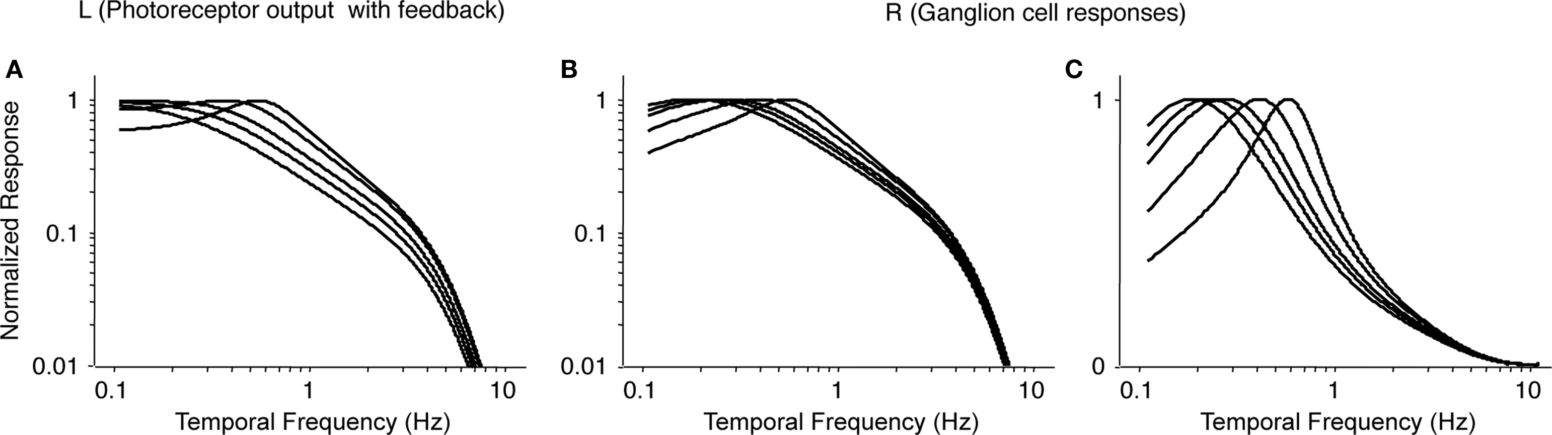
Figure 8. Modeled ganglion cell responses at increasing levels of light adaptation. (A) Transfer functions for photoreceptor output (L, Eq. 6) at increasing levels of light adaptation (i.e., increasing levels of horizontal cell feedback), taken from Figure 7
C. (B) Transfer functions for ganglion cell responses (R, Eq. 11), obtained by high-pass filtering the curves in (A). (C) Same as (B), but plotted on semilog coordinates. These curves are reproduced in Figure 2
of the main text. From left to right within each panel, values of feedback strength are: g = 0, 0.1, 0.2, 0.5, and 1.0.
To summarize: Using the data of Schneeweis and Schnapf (2000)
as the starting point, we showed that, as horizontal cell feedback strength increases, the tuning of the photoreceptor and, ultimately, the ganglion cell, shifts to higher frequencies. As shown in Figure 8
C, the peak frequency shift is approximately 3-fold and can be accounted for by a 10-fold change in horizontal cell feedback strength. Since the shift we present in the main text (Figure 3
C) is a subset of this, a 10-fold change in feedback strength is more than sufficient to account for it.
In the next section, we show how the measured changes in gap junction coupling are sufficient to produce the changes in feedback strength (an expansion of the analysis presented in Materials and Methods).
We conclude the section by mentioning that the analysis done here focused on rod conditions, that is, rod responses were shown with various levels of horizontal cell feedback. We focused on rod conditions, since these are directly compared in the main figure of the paper, Figure 3
C. Specifically, Figure 3
C compares the rod condition in the high feedback state (the state in the knockout in the dark, where horizontal cells are forced to remain uncoupled) with the low feedback state (the state in the wild-type in the dark, where horizontal cells are maximally coupled).
Section B
In this section we detail the relationship between changes in gap junction coupling and horizontal cell feedback strength, an expansion of the description in the Materials and Methods section “The Relation of Horizontal Cell Input Resistance to Coupling for Scotopic Versus Photopic Conditions and for Wild-type Versus Knockout Animals”. We show that the measured changes in coupling are sufficient to produce a 10-fold change in feedback strength and thus are sufficient to account for our results and also for the larger range of shifts shown in Figure 8
C.
As mentioned in “Materials and Methods,” the standard measure of horizontal cell coupling is the length constant. The strength of the horizontal cell signal, on the other hand, is determined by the cell’s input resistance, since the cell’s voltage response is the input resistance multiplied by the input current (Ohm’s law). Thus, to determine how much the horizontal signal changes, we need to determine how much of a change in input resistance is produced by a measured change in length constant.
This is readily accomplished with a well-known model of the horizontal cell network, the two-dimensional cable (Naka and Rushton, 1967
; Lamb, 1976
; Xin and Bloomfield, 1999
; Packer and Dacey, 2005
; Shelley et al., 2006
). We use the two-dimensional cable model to link horizontal cell coupling and length constant, and then to link length constant and input resistance. As we will show, input resistance is inversely proportional to the square of the length constant (for a point source of current, but see also Section C). Xin and Bloomfield (1999)
measured length constants under different degrees of coupling. Their results showed that length constant increases by a factor of 3 between the minimally- and maximally-coupled states. A 3-fold increase in length constant corresponds to a 9-fold decrease in feedback strength, nearly the 10-fold change needed to account for the complete range of shifts in Figure 8
C.
The following details the link between horizontal cell coupling and length constant, and then the link between length constant and input resistance. We focus on the regime in which capacitative effects can be neglected, since the phenomena of interest occur below 2 Hz. At the end of Section D, we comment on how the analysis can be extended to include capacitative effects.
As mentioned above, we start by modeling the horizontal cells as a two-dimensional sheet, as is standard (Naka and Rushton, 1967
; Lamb, 1976
; Xin and Bloomfield, 1999
; Packer and Dacey, 2005
; Shelley et al., 2006
). Within this sheet, horizontal cell coupling determines resistance to current flow, and we denote the sheet resistance by Rs. Thus, our immediate goal is to link Rs to length constant, denoted by λ.
This linkage is well-known, and is given by the classic work of Lamb (1976)
. As Lamb showed (his Eq. 2) the length constant of a two-dimensional sheet is given by

corresponding to Eq. 1 in the main text. Rearranging this yields

corresponding to Eq. 2. Equation 13 demonstrates the relationship between length constant λ and horizontal cell coupling, as measured by the sheet resistance Rs.
The next step is to link input resistance to length constant. We start with a point source current, and consider other geometries in Sections C and D. For a point source current, we begin with Lamb (1976)
(his Eq. 8), which provides the voltage response of the sheet. At a distance r from the injection of a current i0, the resulting voltage V(r) is

where K0 is a modified Bessel function of the second kind.
Input resistance is the ratio of the voltage response to the injected current. At a distance r from the point source, the ratio Zr = V(r)/i0 is

which follows from Eq. 14.
We would like to use Eq. 15 to determine Zr at r = 0 (the point of injection), and how it depends on the horizontal cell parameters. Since the Bessel function in Eq. 15 diverges at the origin, Z0 is formally undefined. However, real measurements correspond to values of r that are small but not 0. Therefore, instead of focusing on Z0, we focus on the limiting behavior of Zr when r is small
2
.
To determine the behavior in the small-r limit, we approximate the Bessel function in Eq. 15, whose argument is u = r/λ. When this argument is small (i.e., when r << λ), the Bessel function has an asymptotic expansion, K0(u) = −(ln u) [1 + o(u)] (Abramowitz and Stegun, 1965
, Eq. 9.6.54). Therefore,

In the small-r limit, the −ln(r)-term grows, eventually dominating the ln(λ)-term, Thus, Zr has an asymptotic expansion

Equation 17 shows that in the limit of a point current injection, input resistance and sheet resistance are proportional (corresponding to the comment following text Eq. 2). Finally, we use the relationship between sheet resistance and length constant (Eq. 13) to rewrite Eq. 17 as

Thus, in the small-r limit, the input resistance is proportional to Rm and inversely proportional to λ2, as in text Eq. 3:

To summarize: horizontal cell coupling (sheet resistance) determines the length constant via Eq. 12, and these are linked to input resistance via Eqs 17 and 18.
Section C
Above, we considered the input resistance for a point input source; we now turn to consider other spatial patterns. To do this systematically, we determine the input resistance for spatial grating pattern of spatial frequency k, which we denote Z(k). That is, Z(k) is the ratio of the voltage response to an applied grating-shaped current. We determine this voltage response by first determining the response to a current injected along a narrow line. Then we superimpose a continuum of line sources to form the grating.
In the scenario of a current injected along a narrow line (say, along the y-axis) into a sheet in the (x, y)-plane, there is translational symmetry along the y-axis. Along the x-axis, the problem reduces to that of a one-dimensional cable. (This is the geometry considered by Xin and Bloomfield, 1999
). Thus, we can use standard one-dimensional cable theory to determine the resulting voltage distribution: at a distance x from a line of injected current I0, the resulting voltage distribution is:

where

is the input resistance of the equivalent one-dimensional cable (Koch and Segev, 1998
).
Next, we create a grating from these line sources. At each location x0 along the x-axis, we place a source with strength I(x0;k) = I0cos(kx0); the net result of these sources is a spatial grating of current. Each of these sources yields a voltage response according to Eq. 20, and they superimpose to yield the voltage response to the grating. Specifically, the contribution of the line source at position x0 to the voltage at position x isVline(x − x0)cos(kx0), and superimposing them yields the grating response:

Carrying out this Fourier integral yields

Thus, Z(k), the input resistance for a current injection patterned as a sinusoid of spatial frequency k, is the ratio of the voltage response to the applied current:

where we have used Eqs 12 and 21 in the last step.
Equation 24 shows how length constant and spatial frequency interact to determine the input resistance. At sufficiently low spatial frequencies, the shunt current has nowhere to go, so the input resistance is Rm, independent of the length constant. At sufficiently high frequencies, the shunt is very effective: input resistance is inversely proportional to λ2, just as in the point source. For example, at k = 3/λ, Z(k) = Rm/10, indicating that 90% of the input resistance can be shunted away, while at k = 1/λ, Z(k) = Rm/2, indicating that half of the input resistance can be shunted away. Since spatial frequency k is measured in radians, the latter corresponds to a spatial wavelength of 2πλ. Thus, perhaps counterintuitively, Eq. 24 shows that the shunt retains effectiveness even for a grating pattern whose period is a fairly large multiple (2π) of the length constant.
To summarize: the reduction in input resistance due to gap junction coupling diminishes at low spatial frequencies, but the falloff is gentle, as shown in Eq. 24. For gratings whose period is small in comparison to 2πλ, the shunt remains large. This was the case in the present experiments under scotopic conditions. We used gratings of 0.039 cycles/degree, corresponding to a spatial period of 795 μm [in the mouse retina, 1° = 31 μm (Remtulla and Hallett, 1985
)], and a spatial frequency k of 2π/795 = 0.0079 μm−1. Given the estimated scotopic length constant of λ = 300 μm (see Stimulating and Recording Ganglion Cell Responses), Eq. 24 yields Z(k) = 0.15Rm, indicating that 85% of the signal can be shunted away.
We conclude by mentioning that while the interaction of spatial pattern and gap junction coupling is a potentially interesting topic, the paper focused on temporal processing and, thus, was not set up to explore this: this is because of a limitation in the size of the retinal pieces used for the multi-electrode array recording. To test the predictions in Eq. 24, retinal pieces of greater than twice the size would be needed to avoid edge effects (shunting through contact with the edge of the retinal piece) and to allow sampling of sufficiently low spatial frequencies. We included the above discussion of the theoretical effects of spatial pattern in any case, because it makes predictions for future work, both in retina and other brain areas where gap junction coupled networks are present.
Section D
Because the gap-junction switch has the potential to operate in a wide range of neural networks, here we briefly note how the above considerations generalize to geometries not directly related to the horizontal cell network of the retina.
First, we mention that the notion that gap junction conductance modulates input resistance is not limited to situations in which the gap-junction-coupled cells form part of a feedback loop. That is, opening the gap junctions of a group of neurons is simply a general way to reduce their gain and thus remove them functionally from a network, whatever their role.
For networks within the brain parenchyma, a three-dimensional space-filling network may be a more appropriate caricature than a two-dimensional syncytial sheet. (We have in mind a scenario in which each neuron is connected to its neighbors in all three spatial dimensions, but that only a part of the volume is occupied by these neurons.) In this case, the dependence of input resistance on gap junction coupling is  , an even stronger dependence than the proportionality which holds in two-dimensional case, Eq. 17.
, an even stronger dependence than the proportionality which holds in two-dimensional case, Eq. 17.To see this, we apply a dimensional analysis. In three dimensions, the resistance Rm to the bath (i.e., extracellular space) has units of ohm-cm3, and the internal resistance, Rs, has units of ohm-cm. Thus, the input resistance for a point source must be proportional to  since this is the only parameter combination that has units of ohms. The length constant λ is still
  , so the input resistance is also proportional to
since this is the only parameter combination that has units of ohms. The length constant λ is still , so the input resistance is also proportional to There is a simple intuition behind this result and the corresponding ones results in the earlier sections: for a point source, the input resistance decreases in proportion to the number of neurons to which an input current spreads. In a “cable” of effective dimension D and length constant λ, this number is proportional to λD.
Finally, we mention that in all of the above analyses, we have considered the gap-junction-coupled network to be purely resistive. This is a reasonable approximation for the experiments considered here: the phenomena of interest occur below 2 Hz. These frequencies are much slower than the estimated RC time constant for the horizontal cell, which is 20 ms, based on membrane resistance and capacitance values provided by Smith (1995)
. Nevertheless, our treatment immediately generalizes to scenarios in which capacitive effects become relevant, by replacing the resistance parameters Rm, Rs, and Z by corresponding frequency-dependent impedances (Koch and Poggio, 1985
). The cable formalism still applies, but now, the effective length constant will be frequency-dependent, and the shunt may be associated with a phase shift.
Figures Un-Normalized
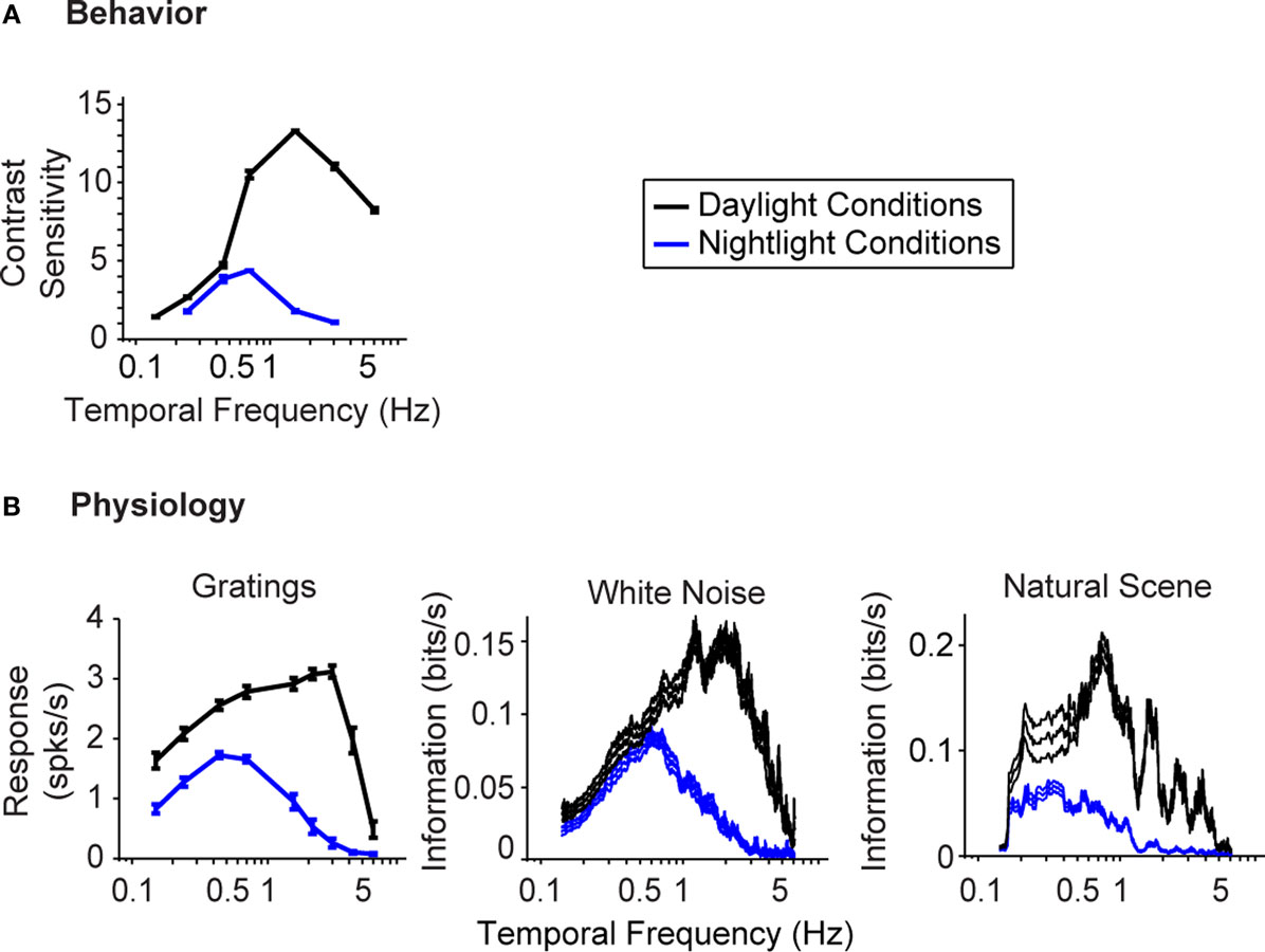
Figure 9. The visual system undergoes a shift in integration time as it shifts from day to night (photopic to scotopic) conditions. This figure reproduces the data in Figure 1
of the main text, but un-normalized. Note that in the un-normalized plots, the shift in tuning to low temporal frequencies is superimposed on an overall decrease in sensitivity, as is well-known at the behavioral level Kelly, 1961
(human); Umino et al., 2008
(mouse)] and at the ganglion cell level (Purpura et al., 1990
).
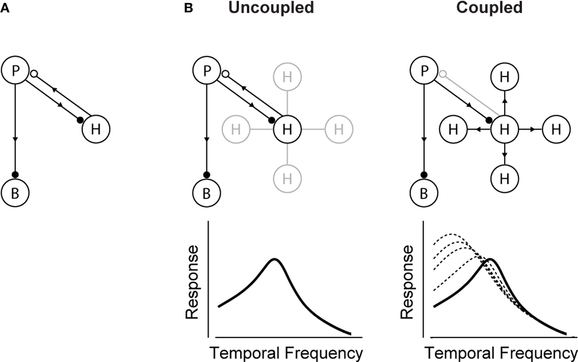
Figure 10. The circuit that controls visual integration time can be shifted from one state to another by a change in the gap junction coupling of one of its cell classes. This figure reproduces the model shown in the main text, but with the response curves un-normalized (see Figure 2
of the main text or Figure 8
C of Appendix 2).
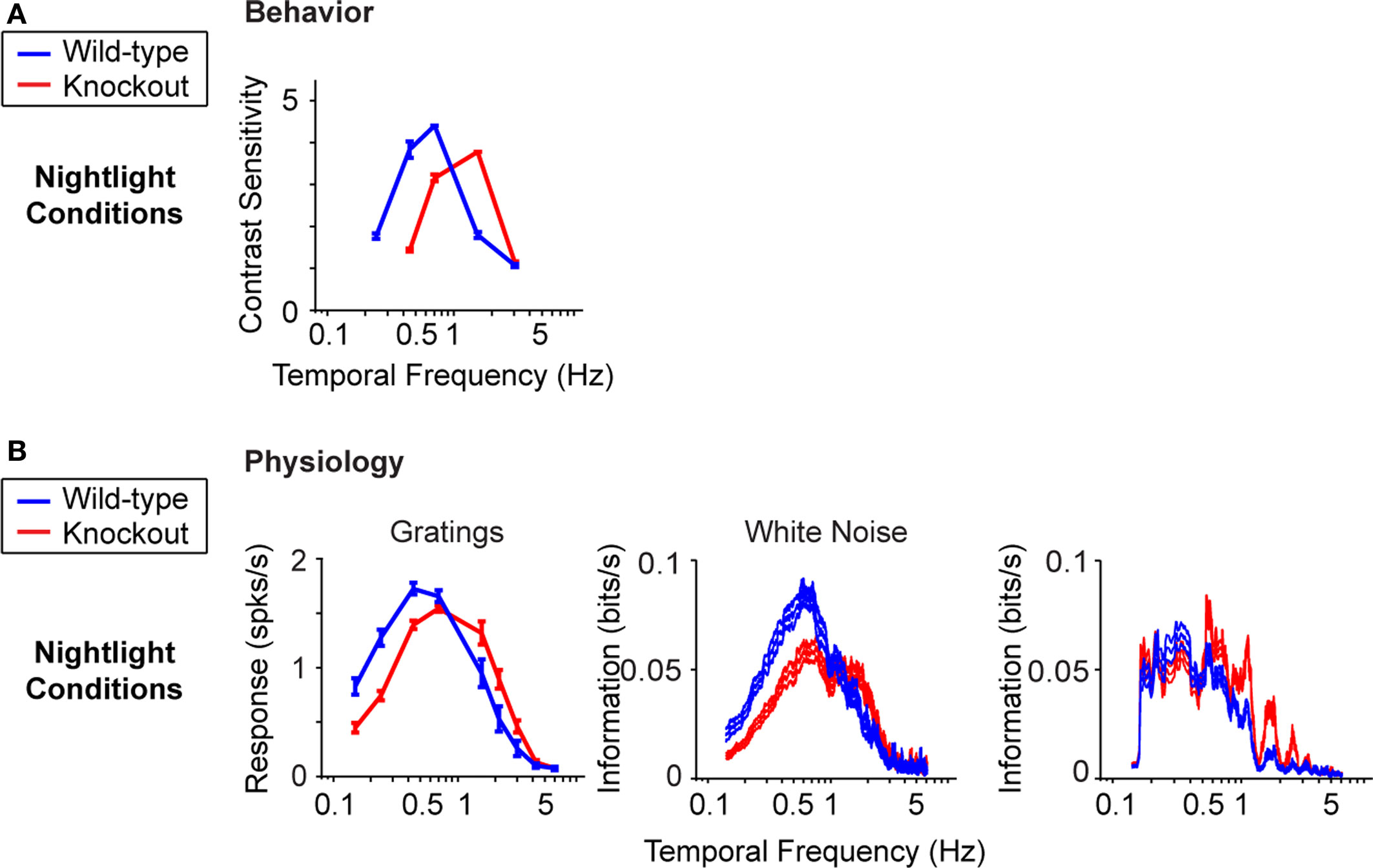
Figure 11. When coupling is prevented, the shift to long integration times is impaired at both the behavioral level and the ganglion cell level. This figure reproduces the data in Figure 3
of the main text, but un-normalized. As in the main text, the knockout response fails to make the normal shift in tuning to low temporal frequencies, because the feedback signal is not reduced by the shunt. Note that the un-normalized plots show that at low temporal frequencies, the wild-type response is higher, while at high temporal frequencies, the knockout response is higher. This is predicted by the model (Figure 10
, which shows the un-normalized model predictions; lower right of figure). Note also that this crossover (the higher response in the no-feedback state at low frequencies, and the higher response in the high-feedback state at high frequencies) is a well-known phenomenon in light adaptation (Purpura et al., 1990
).
The authors declare that the research was conducted in the absence of any commercial or financial relationships that could be construed as a potential conflict of interest.
We thank A. Molnar for helpful discussion, Y. Roudi, and K. Purpura for comments on the manuscript, and K. Willecke and colleagues for the use of the Cx57lacZ/lacZ mouse line. Figure 3
A was adapted from a previous paper by our group, Dedek et al. (2008)
. This work was supported by funds from National Eye Institute R01 EY12978 to S. Nirenberg; C. Pandarinath was supported in part by T32-EY07138; J. Victor is supported in part by funds from National Eye Institute RO1 EY7977 and EY9314”.
The Supplementary Material for this article can be found online at http://www.frontiersin.org/computationalneuroscience/paper/10.3389/fncom.2010.00002
Filtered Movies
The selective disadvantage of a Cx57 gene loss, demonstrated using a natural movie
As indicated in the main text, we filmed an approaching predator and restricted the movies to the temporal frequencies available to each genotype, using the data from Figure 3
D left. In Figure 4
we showed single frames from the movies; here we show the movies in total. As indicated in the main text, in daytime conditions, the movies for the two genotypes are essentially the same – see Video 1, Wild-type by Day, and Video 2, Knockout by Day. In nighttime conditions, though, the two movies diverge. In the movie filtered through the frequencies visible to the wild-type animal, the predator is visible both when it is moving, i.e., when the movie is dominated by high frequencies, and when it is still, i.e., when the movie is dominated by low frequencies. In the movie filtered though the frequencies visible to the knockout, the predator disappears in the still condition. Only a ghost remains – see Video 3, Wild-type at Night, and Video 4, Knockout at Night.
Janssen-Bienhold, U., Trumpler, J., Hilgen, G., Schultz, K., De Sevilla Muller, L., Sonntag, S., Dedek, K., Dirks, P., Willecke, K., and Weiler, R. (2009). Connexin57 is expressed in dendro-dendritic and axo-axonal gap junctions of mouse horizontal cells and its distribution is modulated by light. J. Comp. Neurol. 513, 363–374.