Department of Mathematics, College of Natural Sciences and Mathematics, University of Houston, Houston, TX, USA
Correlations between spike trains can strongly modulate neuronal activity and affect the ability of neurons to encode information. Neurons integrate inputs from thousands of afferents. Similarly, a number of experimental techniques are designed to record pooled cell activity. We review and generalize a number of previous results that show how correlations between cells in a population can be amplified and distorted in signals that reflect their collective activity. The structure of the underlying neuronal response can significantly impact correlations between such pooled signals. Therefore care needs to be taken when interpreting pooled recordings, or modeling networks of cells that receive inputs from large presynaptic populations. We also show that the frequently observed runaway synchrony in feedforward chains is primarily due to the pooling of correlated inputs.
Cortical neurons integrate inputs from thousands of afferents. Similarly, a variety of experimental techniques record the pooled activity of large populations of cells. It is therefore important to understand how the structured response of a neuronal network is reflected in the pooled activity of cell groups.
It is known that weak dependencies between the response of cell pairs in a population can have a significant impact on the variability and signal-to-noise ratio of the pooled signal (Shadlen and Newsome, 1998
; Salinas and Sejnowski, 2000
; Moreno-Bote et al., 2008
). It has also been observed that weak correlations between cells in two populations can cause much stronger correlations between the pooled activity of the populations (Bedenbaugh and Gerstein, 1997
; Chen et al., 2006
; Gutnisky and Josić, 2010
; Renart et al., 2010
). We give a simple example of this effect in Figure 1
C: Weak correlations were introduced between the spiking activity of cells in two non-overlapping presynaptic pools each providing input to a postsynaptic cell (see diagram in Figure 1
B). The activity between pairs of excitatory, and pairs of inhibitory cells was correlated, but excitatory–inhibitory pairs were uncorrelated. Even without shared inputs and with background noise, pooling resulted in strong correlations in postsynaptic membrane voltages. The connectivity in the presynaptic network was irrelevant – it only mattered that the inputs to the downstream neurons reflected the pooled activity of the afferent populations. A similar effect can cause large correlations between recordings of multiunit activity (MUA) or recordings of voltage sensitive dyes (VSD), even when correlations between cells in the recorded populations are small (Bedenbaugh and Gerstein, 1997
; Chen et al., 2006
; Stark et al., 2008
). The effect is the same, but in this case pooling occurs at the level of a recording device rather than a downstream neuron (compare Figures 1
A,B).
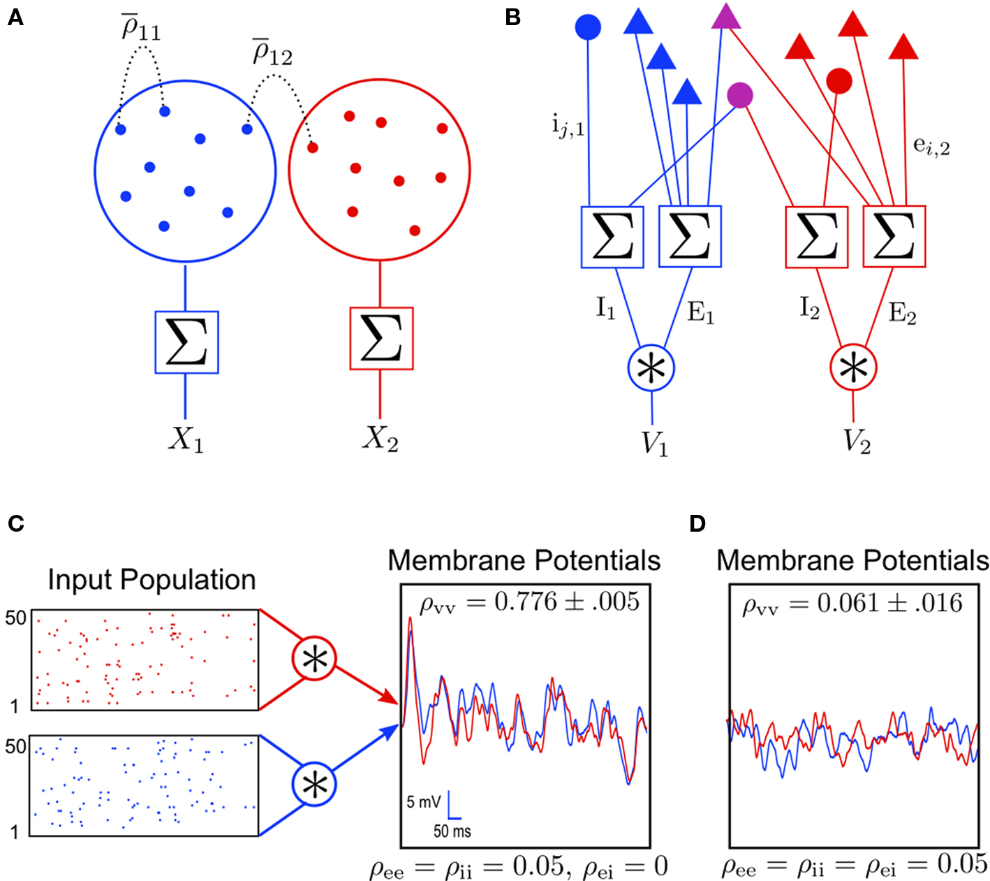
Figure 1. Models of pooled recordings and the effects of pooling on correlations. (A) Pooling in experimental recordings. Cells from different populations are correlated with average correlation coefficient  and cells from the same population have average correlation coefficient
  or
or  We examine correlations between the pooled signals, X1 and X2. (B) Pooled inputs to cell pairs. Individual excitatory (e) and inhibitory (i) inputs are correlated with coefficient ρee, ρii, and ρei, respectively. The total input to a cell is the summed activity of its excitatory (EK) and inhibitory (IK) presynaptic population. The membrane potentials, V1 and V2, are obtained by filtering these inputs. (C) A simulation of the setup in (B) with background noise. Correlations between excitatory and between inhibitory cells were uniform (ρee = ρii = 0.05), but excitatory–inhibitory correlations were absent (ρei = 0). The raster plot shows the activity in a subset of the input population. The correlation coefficient between the sub-threshold activity of the postsynpatic cells was ρvv = 0.768 ± 0.001 s.e. Each cell receives 250 correlated and 250 uncorrelated excitatory Poisson inputs as well as 84 correlated and 84 uncorrelated inhibitory Poisson inputs (ne = 250 and ni = 84, qe = qi = 1, νe = 5 Hz, νi = 7.5 Hz, ℐ = 4ℰ, and ℰ≈2.3 nS·ms – see Materials and Methods and Figure 3
A for notation and precise model description). (D) Same as (B), but with ρei = 0.05, νe = νi=5 Hz, ℐ = 6ℰ to maintain balance. In this case ρVV = 0.0085 ± 0.0024 s.e.. The simulations were run 8000 times at 10 s each.
We examine correlations between the pooled signals, X1 and X2. (B) Pooled inputs to cell pairs. Individual excitatory (e) and inhibitory (i) inputs are correlated with coefficient ρee, ρii, and ρei, respectively. The total input to a cell is the summed activity of its excitatory (EK) and inhibitory (IK) presynaptic population. The membrane potentials, V1 and V2, are obtained by filtering these inputs. (C) A simulation of the setup in (B) with background noise. Correlations between excitatory and between inhibitory cells were uniform (ρee = ρii = 0.05), but excitatory–inhibitory correlations were absent (ρei = 0). The raster plot shows the activity in a subset of the input population. The correlation coefficient between the sub-threshold activity of the postsynpatic cells was ρvv = 0.768 ± 0.001 s.e. Each cell receives 250 correlated and 250 uncorrelated excitatory Poisson inputs as well as 84 correlated and 84 uncorrelated inhibitory Poisson inputs (ne = 250 and ni = 84, qe = qi = 1, νe = 5 Hz, νi = 7.5 Hz, ℐ = 4ℰ, and ℰ≈2.3 nS·ms – see Materials and Methods and Figure 3
A for notation and precise model description). (D) Same as (B), but with ρei = 0.05, νe = νi=5 Hz, ℐ = 6ℰ to maintain balance. In this case ρVV = 0.0085 ± 0.0024 s.e.. The simulations were run 8000 times at 10 s each.
and cells from the same population have average correlation coefficient or We examine correlations between the pooled signals, X1 and X2. (B) Pooled inputs to cell pairs. Individual excitatory (e) and inhibitory (i) inputs are correlated with coefficient ρee, ρii, and ρei, respectively. The total input to a cell is the summed activity of its excitatory (EK) and inhibitory (IK) presynaptic population. The membrane potentials, V1 and V2, are obtained by filtering these inputs. (C) A simulation of the setup in (B) with background noise. Correlations between excitatory and between inhibitory cells were uniform (ρee = ρii = 0.05), but excitatory–inhibitory correlations were absent (ρei = 0). The raster plot shows the activity in a subset of the input population. The correlation coefficient between the sub-threshold activity of the postsynpatic cells was ρvv = 0.768 ± 0.001 s.e. Each cell receives 250 correlated and 250 uncorrelated excitatory Poisson inputs as well as 84 correlated and 84 uncorrelated inhibitory Poisson inputs (ne = 250 and ni = 84, qe = qi = 1, νe = 5 Hz, νi = 7.5 Hz, ℐ = 4ℰ, and ℰ≈2.3 nS·ms – see Materials and Methods and Figure 3
A for notation and precise model description). (D) Same as (B), but with ρei = 0.05, νe = νi=5 Hz, ℐ = 6ℰ to maintain balance. In this case ρVV = 0.0085 ± 0.0024 s.e.. The simulations were run 8000 times at 10 s each.We present a systematic overview, as well as extensions and applications of a number of previous observations related to this phenomenon. Using a linear model, we start by examining the potential effects of pooling on recordings from large populations obtained using VSD or MUA recording techniques. These techniques are believed to reflect the pooled postsynpatic activity of groups of cells. We extend earlier models introduced to examine the impact of pooling on correlations (Bedenbaugh and Gerstein, 1997
; Chen et al., 2006
; Nunez and Srinivasan, 2006
), and show that heterogeneities in the presynaptic pools can have subtle effects on correlations between pooled signals.
Since neurons respond to input from large presynaptic populations, pooling also impacts the activity of single cells and cell pairs. As observed in Figure 1
C, pooling can inflate weak correlations between afferents. However, excitatory–inhibitory correlations (Okun and Lampl, 2008
) can counteract this amplification, as shown in Figure 1
D (Hertz, 2010
; Renart et al., 2010
). We examine these effects analytically by modeling the subthreshold activity of postsynaptic cells as a filtered version of the inputs received (Tetzlaff et al., 2008
). The impact of correlated subthreshold activity on the output spiking statistics is a nontrivial question which we address only briefly (Moreno-Bote and Parga, 2006
; de la Rocha et al., 2007
; Ostojić et al., 2009
).
The effects of pooling provide a simple explanation for certain aspects of the dynamics of feedforward chains. Simulations and in vitro experiments show that layered feedforward architectures give rise to a robust increase in synchronous spiking from layer to layer (Diesmann et al., 1999
; Litvak et al., 2003
; Reyes, 2003
; Doiron et al., 2006
; Kumar et al., 2008
). We describe how output correlations in one layer impact correlations between the pooled inputs to the next layer. This approach is used to derive a mapping that describes how correlations develop across layers (Tetzlaff et al., 2003
; Renart et al., 2010
), and to illustrate that the pooling of correlated inputs is the primary mechanism responsible for the development of synchrony in feedforward chains. Examining how correlations are mapped between layers also helps explain why asynchronous states are rarely observed in feedforward networks in the absence of strong background noise (van Rossum et al., 2002
; Vogels and Abbott, 2005
). This is in contrast to recurrent networks which can display stable asynchronous states (Hertz, 2010
; Renart et al., 2010
) similar to those observed in vivo (Ecker et al., 2010
).
Correlations Between Stochastic Processes
The cross-covariance of a pair of stationary stochastic processes, x(t) and y(t), is Cxy(t) = cov(x(s), y(s + t)). The auto-covariance function, Cxx(t), is the cross-covariance between a process and itself. The cross- and auto-covariance functions measure second order dependencies at time lag t between two processes, or a process and itself. We quantify the total magnitude of interactions over all time using the asymptotic statistics,
While the asymptotic correlation, ρxy, measures correlations between x(t) and y(t) over large timescales, the auto- and cross-covariance functions determine the timescale of these dependencies.
Correlations Between Sums of Random Variables
Given two collections of correlated random variables  and
and  define the pooled variables,
  and
and  Since covariance is bilinear
  the variance and covariance of the pooled variables are
and define the pooled variables, and Since covariance is bilinear the variance and covariance of the pooled variables are
and similarly for 
Using these expressions along with some algebraic manipulation, the correlation coefficient,  between the pooled variables can be written as
between the pooled variables can be written as
where
and similarly for wy, vy,  and
and  In deriving Eq. (3) we assumed that all pairwise statistics are uniformly bounded away from zero in the asymptotic limit.
and In deriving Eq. (3) we assumed that all pairwise statistics are uniformly bounded away from zero in the asymptotic limit.Each overlined term above is a population average. Notably,  represents the average correlation between xi and yj pairs, weighted by the product of their standard deviations, and similarly for
  and
and  Correlation between weighted sums can be obtained by substituting
  and
and  for weights
  and
and  and making the appropriate changes to the terms in the equation above (e.g.,
 ). Overlap between the two populations can be modeled by taking
  for some pairs.
represents the average correlation between xi and yj pairs, weighted by the product of their standard deviations, and similarly for and Correlation between weighted sums can be obtained by substituting and for weights and and making the appropriate changes to the terms in the equation above (e.g.,). Overlap between the two populations can be modeled by taking for some pairs.Assuming that variances are homogeneous within each population, that is  and
and  for i = 1,…,nx and j = 1,…,ny, simplifies these expressions. In particular,
 and
and
and for i = 1,…,nx and j = 1,…,ny, simplifies these expressions. In particular, and
Assuming further that the populations are symmetric, σx = σy = σ, nx = ny = n, and  the expression above simplifies to
the expression above simplifies to
where  is the average pairwise correlation between the two populations and
  is the average pairwise correlation within each population. Eq. (5) was derived in Bedenbaugh and Gerstein (1997)
in an examination of correlations between multiunit recordings. In Chen et al. (2006)
, a version of Eq. (5) with ρw = ρb is derived in the context of correlations between two VSD signals. The asymptotic, ρxy → 0, limit when ρw = ρb is discussed in Renart et al. (2010)
.
is the average pairwise correlation within each population. Eq. (5) was derived in Bedenbaugh and Gerstein (1997)
in an examination of correlations between multiunit recordings. In Chen et al. (2006)
, a version of Eq. (5) with ρw = ρb is derived in the context of correlations between two VSD signals. The asymptotic, ρxy → 0, limit when ρw = ρb is discussed in Renart et al. (2010)
.
is the average pairwise correlation between the two populations and is the average pairwise correlation within each population. Eq. (5) was derived in Bedenbaugh and Gerstein (1997)
in an examination of correlations between multiunit recordings. In Chen et al. (2006)
, a version of Eq. (5) with ρw = ρb is derived in the context of correlations between two VSD signals. The asymptotic, ρxy → 0, limit when ρw = ρb is discussed in Renart et al. (2010)
.Note that the results above hold for correlations computed over arbitrary time windows. We concentrate on infinite windows, and discuss extensions in the Appendix.
Neuron Model
In the second part of the presentation we consider two excitatory and two inhibitory input populations projecting to two postsynaptic cells. The jth excitatory input to cell k is labeled ej,k(t) (k = 1 or 2). Similarly, ij,k(t) denotes the jth inhibitory input to cell k. Each cell receives ne excitatory and ni inhibitory inputs with individual rates νe and νi respectively.
Each of the excitatory and inhibitory inputs to cell k, are stationary spike trains modeled by point processes,  and
and  where
where  and
and  are input spike times. We assume that the spike trains are stationary in a multivariate sense (Stratonovich, 1963
). The pooled excitatory and inhibitory inputs to neuron k are
are input spike times. We assume that the spike trains are stationary in a multivariate sense (Stratonovich, 1963
). The pooled excitatory and inhibitory inputs to neuron k are  and
and 
and where and are input spike times. We assume that the spike trains are stationary in a multivariate sense (Stratonovich, 1963
). The pooled excitatory and inhibitory inputs to neuron k are and To generate correlated inputs to cells, we used the multiple interaction process (MIP) method (Kuhn et al., 2003
), then jittered each spike time independently by a random value drawn from an exponential distribution with mean 5ms. The resulting processes are Poisson with cross-covariance functions proportional to a double exponential, Cxy(t) ∼ e− |t| /5. Note that since each input is Poisson,  and
and 
and While the dynamics of the afferent population were not modeled explicitly, the response of the two downstream neurons was obtained using a conductance-based IF model. The membrane potentials of the neurons were described by

with excitatory and inhibitory conductances determined by  and
and  where * denotes convolution. We used synaptic responses of the form
  and
and  where Θ(t) is the Heaviside function. The area of a single excitatory or inhibitory postsynaptic conductance (EPSC or IPSC) is therefore equal to the synaptic weight, ℰ or ℐ, with units nS·ms. This analysis can easily be extended to situations where each input, ej,k or ij,k, has a distinct synaptic weight.
and where * denotes convolution. We used synaptic responses of the form and where Θ(t) is the Heaviside function. The area of a single excitatory or inhibitory postsynaptic conductance (EPSC or IPSC) is therefore equal to the synaptic weight, ℰ or ℐ, with units nS·ms. This analysis can easily be extended to situations where each input, ej,k or ij,k, has a distinct synaptic weight.When examining spiking activity, we assume that when Vk crosses a threshold voltage, Vth, an output spike is produced and Vk is reset to VL. When examining sub-threshold dynamics, we considered the free membrane potential without threshold.
As a measure of balance between excitation and inhibition we used (Troyer and Miller, 1997
; Salinas and Sejnowski, 2000
)
When β = 1, the net excitation and inhibition are balanced and the mean free membrane potential equals VL. In simulations, we set VL = −60 mV, VE = 0 mV, VI = −90 mV, τe = 10 ms, τi = 20 ms, Cm = 114 pF, and gL = 4.086 nS, giving a membrane time constant, τm = Cm/gL = 27.9 ms. In all simulations except those in Figure 7
, the cells are balanced (β = 1).
The conductance-based IF neuron behaves as a nonlinear filter in the sense that membrane potentials cannot be written as a linear transformation of the inputs. However, following Kuhn et al. (2004) and Coombes et al. (2007)
, we derive a linear approximation to the conductance based model. Let U = Vk − VL so that Eq. (6) becomes

Define the effective membrane time constant, τeff Cm/(E[gL+gE(t) + gL(t)]) Cm/(gL+ neveℰ + niviℐ Substituting this average value in the previous equation yields the linear approximation to the conductance based model,

where  is the total input current to cell k. Solving and reverting to the original variables gives the linear approximation Vk(t) = (Jk*K)(t) + VL, where
  is the kernel of the linear filter induced by Eq. (7).
is the total input current to cell k. Solving and reverting to the original variables gives the linear approximation Vk(t) = (Jk*K)(t) + VL, where is the kernel of the linear filter induced by Eq. (7).The pooling of signals from groups of neurons can impact both recordings of population activity and the structure of inputs to postsynaptic cells. We start by discussing correlations in pooled recordings using a simple linear model. A similar model is then used to examine the impact of pooling on the statistics of inputs to cells. For simplicity we assume that all spike trains are stationary. However, non-stationary results can be obtained using similar methods as outlined in the Section “Discussion.” Though all parameters are defined in the Meterials and Methods, Tables 1 and 2
in the Appendix contain brief descriptions of parameters for quick reference. Also, Tables 3 and 4
summarize the values of parameters used for simulations throughout the article.
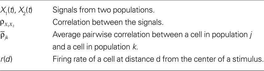
Table 1. Definitions of variables pertaining to recordings.
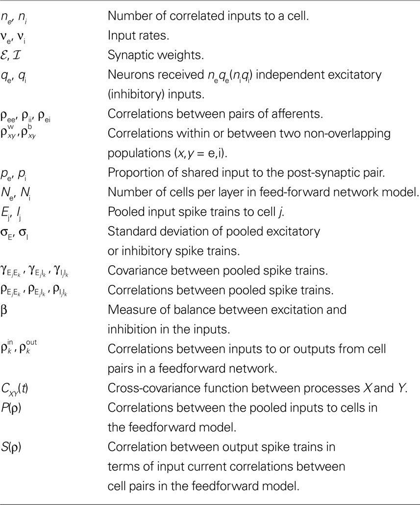
Table 2. Definitions of variables pertaining to downstream cells. Subscripts e and E (i and I) denote excitation (inhibition).
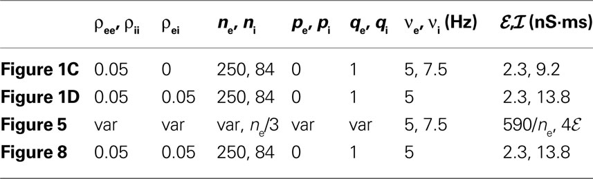
Table 3. Parameter values for simulations of two downstream cells. For fields with “var,” various values of the indicated parameters were used and are described in the captions. For all simulations, VL = −60 mV, VE = 0 mV, VI = −90 mV, Cm = 114 pF, gL = 4.086 nS, τe = 10 ms, τi = 20 ms.
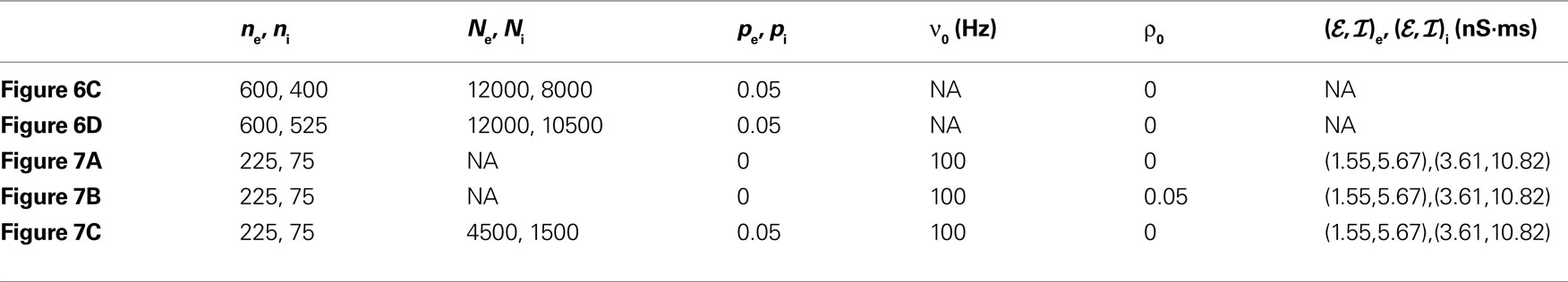
Table 4. Parameter values for simulations of feedforward networks. The parameter υ0 is the input rate to the first layer, (ℰ,ℐ)e indicates synaptic weights for excitatory cells, and (ℰ, ℐ)i for inhibitory cells. For all simulations, VL = −60 mV, VE = 0 mV, VI = −90 mV, Cm = 114 pF, gL = 4.086 nS, τe = 10 ms, τi = 20 ms. For Figure 6
, theoretical values were obtained under the assumption that υe = υ i and ℰ|VE − VL| = ℐ|VI − VL|.
Correlations Between Pooled Recordings
Pooling can impact correlations between recordings of population activity obtained from voltage sensitive dyes (VSDs), multi-unit recordings and other techniques. Such signals might each represent the summed activity of hundreds or thousands of neurons. Let two recorded signals, X1(t) and X2(t), represent the weighted activity of cells in two populations (see diagram in Figure 1
A). If we assume homogeneity in the input variances and equal size of the recorded populations, Eq. (4) gives the correlation between the recorded signals
Here n represents the number of neurons recorded,  k = 1,2 represents the average correlation between cells contributing to signal Xk(t), and represents the average correlation between cells contributing to different signals. The averages are weighted so that cells that contribute more strongly to the recording, such as those closer to the recording site, contribute more to the average correlations (see Materials and Methods). Cells common to both recorded populations can be modeled by setting the corresponding correlation coefficients to unity. A form of Eq. (8) with
  was derived by Bedenbaugh and Gerstein (1997)
.
was derived by Bedenbaugh and Gerstein (1997)
.
k = 1,2 represents the average correlation between cells contributing to signal Xk(t), and represents the average correlation between cells contributing to different signals. The averages are weighted so that cells that contribute more strongly to the recording, such as those closer to the recording site, contribute more to the average correlations (see Materials and Methods). Cells common to both recorded populations can be modeled by setting the corresponding correlation coefficients to unity. A form of Eq. (8) with was derived by Bedenbaugh and Gerstein (1997)
.When the two recording sites are nearby, so that  even small correlations between individual cells are amplified by pooling so that the correlations between the recorded signals can be close to 1. This effect was observed in experiments and explained in similar terms in Stark et al. (2008)
.
even small correlations between individual cells are amplified by pooling so that the correlations between the recorded signals can be close to 1. This effect was observed in experiments and explained in similar terms in Stark et al. (2008)
.
even small correlations between individual cells are amplified by pooling so that the correlations between the recorded signals can be close to 1. This effect was observed in experiments and explained in similar terms in Stark et al. (2008)
.A significant stimulus-dependent change in correlations between individual cells might be reflected only weakly in the correlation between the pooled signals. This can occur, for instance, in recordings of large populations when 
 and are increased by the same factor when a stimulus is presented. Similarly, an increase in correlations between cells can actually lead to a decrease in correlations between recorded signals when and
  increase by a larger factor than
and are increased by the same factor when a stimulus is presented. Similarly, an increase in correlations between cells can actually lead to a decrease in correlations between recorded signals when and increase by a larger factor than To illustrate these effects, we construct a simple model of stimulus dependent correlations motivated by the experiments in Chen et al. (2006)
, in which VSDs were used to record the population response in visual area V1 during an attention task. In their experiments, the imaged area is divided into 64 pixels, each 0.25 mm × .25 mm in size. The signal recorded from each pixel represents the pooled activity of n ≈ 1.25 × 10⁴ neurons.
We model correlations between the signals, X1(t) and X2(t), recorded from two pixels in the presence or absence of a stimulus (see Figure 2
B), using a simplified model of stimulus dependent rates and correlations. The firing rate of a cell located at distance d from the center of the retinotopic image of a stimulus is
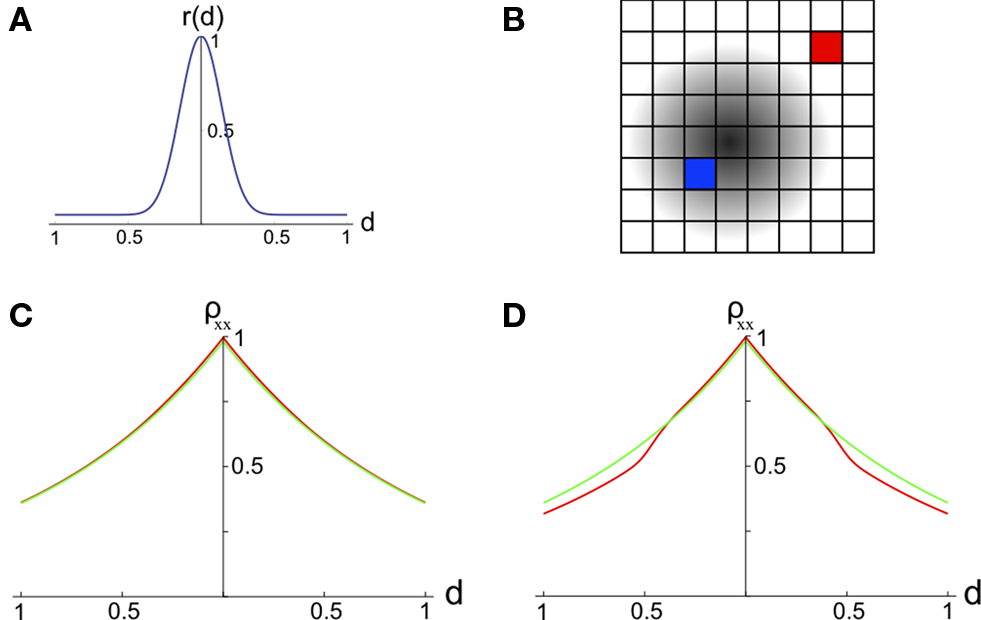
Figure 2. The effect of pooling on recordings of stimulus dependent correlations. (A) The response amplitude of a model neuron as a function of its distance from the retinotopic image of a stimulus [Eq. (9)] with B = 0.05 and λ = 10. (B) A diagram of our model. Signals X1(t) and X2(t) are recorded from two pixels (red and blue squares). The activity in response to a stimulus is shown as a gradient centered at some pixel (the center of the retinotopic image of the stimulus). (C) The prediction of the correlation between two pixels obtained using the stimulus-dependent model considered in the text with stimulus present (red) and absent (green). We assumed that one pixel is located at the stimulus center (d1 = 0). Parameters are as in (A) with α = 1, S = 0.1, and n = 1.25×10⁴. A stimulus dependent change in correlations is undetectable. (D) Same as in (C), except that baseline activity, B, was scaled by 0.5 in the presence of a stimulus. Compare to Figure 2f in Chen et al., 2006
.
Here, B ∈ [0,1] represents baseline activity and λ ≥ 1 controls the rate at which activity decays with d. Both d and r were scaled so that their maximum value is 1 (see Figure 2
A).
We assume that the correlation between the responses of two neurons is proportional to the geometric mean of their firing rates (de la Rocha et al., 2007
; Shea-Brown et al., 2008
), and that correlations decay exponentially with cell distance (Smith and Kohn, 2008
; see however Poort and Roelfsema, 2009
; Ecker et al., 2010
). We therefore model the correlation between two cells as  where dj and dk are the distances from each cell to the center of the retinotopic image of the stimulus, Dj,k is the distance between cells j and k, α is the rate at which correlations decay with distance, and S ≤ 1 is a constant of proportionality.
where dj and dk are the distances from each cell to the center of the retinotopic image of the stimulus, Dj,k is the distance between cells j and k, α is the rate at which correlations decay with distance, and S ≤ 1 is a constant of proportionality.If pixels are small compared to the scales at which correlations are assumed to decay, then the average correlation between cells within the same pixel are  and
and  The average correlation between cells in different pixels is
and The average correlation between cells in different pixels is In this case, whether a stimulus is present or not, the correlation between the pooled signals is of the form  Thus, even significant stimulus dependent changes in correlations would be invisible in the recorded signals. This overall trend is consistent with the results in Chen et al. (2006)
(compare Figure 2
C to their Figure 2f). In such settings, it is difficult to conclude whether pairwise correlations are stimulus dependent or not from the pooled data.
Thus, even significant stimulus dependent changes in correlations would be invisible in the recorded signals. This overall trend is consistent with the results in Chen et al. (2006)
(compare Figure 2
C to their Figure 2f). In such settings, it is difficult to conclude whether pairwise correlations are stimulus dependent or not from the pooled data.However, in Supplementary Figure 3 of Chen et al. (2006
) the presence of a stimulus apparently results in a slight decrease in correlations between more distant pixels. In Figure 2
D this effect was reproduced using the alternative model described above, with the additional assumption that baseline activity, B, decreases in the presence of a stimulus (Mitchell et al., 2009
). The effect can also be reproduced by assuming that spatial correlation decay, α, increases when a stimulus is present.
As this example shows, care needs to be taken when inferring underlying correlation structures from pooled activity. The statistical structure of the recordings can depend on pairwise correlations between individual cells in a subtle way, and different underlying correlation structures may be difficult to distinguish from the pooled signals. However, downstream neurons may also be insensitive to the precise structure of pairwise correlations, as they are driven by the pooled input from many afferents.
Correlations Between the Pooled Inputs to Cells
We next examine the effects of pooling by relating the correlations between the activity of downstream cells to the pairwise correlations between cells in the input populations (see Figure 1
B). The idea that pooling amplifies correlations carries over from the previous section. However, the presence of inhibition and non-instantaneous synaptic responses introduces new issues.
A homogeneous population with overlapping and independent inputs
For simplicity, we first consider a homogeneous population model (see Figure 3
A). Each cell receives ne inputs from a homogeneous pool of inputs with pairwise correlation coefficients ρee and an additional qene inputs from an outside pool of independent inputs. The two cells share pene of the inputs drawn from the correlated pool. Processes in the independent pool are uncorrelated with all other processes. All excitatory inputs have variance 
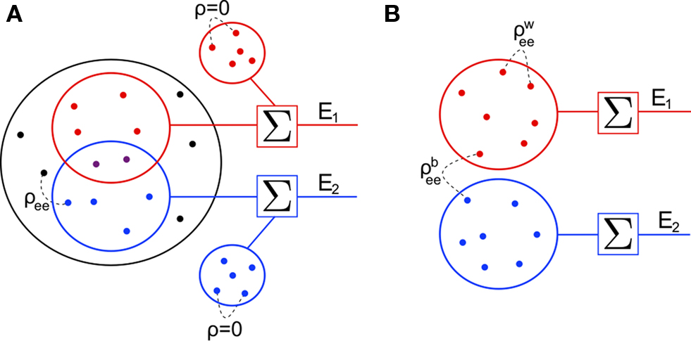
Figure 3. Two population models considered in the text. (A) Homogeneous population with overlap and independent inputs: A homogeneous pool of correlated inputs (large black circle) with correlation coefficient between any pair of processes equal to ρee. Each cell draws ne inputs (larger red and blue circles) from this homogeneous input pool. Of these ne correlated inputs, pene are shared between the two neurons (purple dots). In addition, each cell receives qene independent inputs (smaller red and blue circles), for a total of ne + qene inputs. All inputs have variance (B) A population model with distinct “within” and “between” correlations: Each cell receives ne inputs. The average correlation between two inputs to the same cell  is and between inputs to different cells is
(B) A population model with distinct “within” and “between” correlations: Each cell receives ne inputs. The average correlation between two inputs to the same cell is and between inputs to different cells is The correlation between the pooled excitatory inputs is given by (see Appendix)
A form of this equation, with pe = 0 and qe = 0, is derived in Chen et al. (2006)
. In the absence of correlations between processes in the input pools, ρee = 0, the correlation between the pooled signals is just the proportion of shared inputs,  When ρee > 0 and ne is large, pooled excitatory inputs are highly correlated, even when pairwise correlations in the presynaptic pool, ρee, are small, and the neurons do not share inputs (pe = 0). Even when most inputs to the downstream cells are independent (qe > 1), correlations between the pooled signals will be nearly 1 for sufficiently large input pools (see Figure 4
A).
When ρee > 0 and ne is large, pooled excitatory inputs are highly correlated, even when pairwise correlations in the presynaptic pool, ρee, are small, and the neurons do not share inputs (pe = 0). Even when most inputs to the downstream cells are independent (qe > 1), correlations between the pooled signals will be nearly 1 for sufficiently large input pools (see Figure 4
A).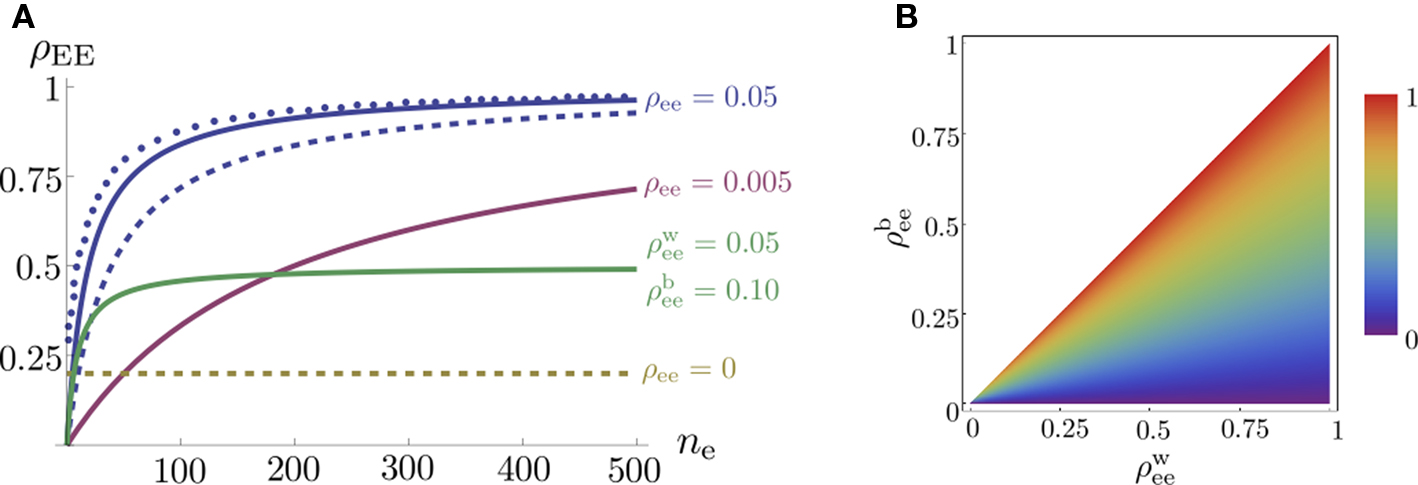
Figure 4. The effect of pooling on correlations between summed input spike trains. (A) The correlation coefficient between the pooled excitatory spike trains (ρEE) is shown as a function of the size of the correlated excitatory input pool (ne) for various parameter settings. The solid blue line was obtained by setting ρee = 0.05 for the population model in Figure 3
A in the absence of shared or independent inputs (pe = qe = 0). The dashed line illustrates the decorrelating effects of the addition of ne independent inputs (qe = 1, qe = 0, ρee = 0.05). The dotted blue line shows that shared inputs increase correlations, but have a diminishing effect on ρEE with increasing input population size (pe = 0.2, qe = 0, ρee = 0.05). The solid pink line shows the effect of reducing the pairwise input correlations (ρee = 0.005, pe = qe = 0). The dashed tan line was obtained with uncorrelated inputs so that correlations reflected shared inputs alone (pe = 0.2, ρee = qe = 0). The green line was obtained with disparity in the “within” and “between” correlations ( and
and  ) using the model in Figure 3
B. (B) The correlations coefficient, ρEE, between the pooled inputs as a function of the within and between correlations (
) using the model in Figure 3
B. (B) The correlations coefficient, ρEE, between the pooled inputs as a function of the within and between correlations ( and
and  ) for ne = 50. Note that the pooled correlation is relatively constant along lines through the origin. Thus, changing
  and
and  by the same proportion does not affect the pooled correlation.
and ) using the model in Figure 3
B. (B) The correlations coefficient, ρEE, between the pooled inputs as a function of the within and between correlations ( and ) for ne = 50. Note that the pooled correlation is relatively constant along lines through the origin. Thus, changing and by the same proportion does not affect the pooled correlation.Under analogous homogeneity assumptions for the inhibitory pools, the correlation, between the pooled inhibitory inputs is given by an equation identical to Eq. (10), and the correlation  between the pooled excitatory and inhibitory inputs is given by
between the pooled excitatory and inhibitory inputs is given by
Interestingly, since  pairwise excitatory–inhibitory correlations obey the bound
  Combining this inequality with Eq. (10) and the analogous equation for
  it follows that
  for homogeneous populations. These are a result of the non-negative definiteness of covariance matrices.
pairwise excitatory–inhibitory correlations obey the bound Combining this inequality with Eq. (10) and the analogous equation for it follows that for homogeneous populations. These are a result of the non-negative definiteness of covariance matrices.Heterogeneity and the effects of spatially dependent correlations
We next discuss how heterogeneity can dampen the amplification of correlations due to pooling. In the absence of any homogeneity assumptions on the excitatory input population (see the population model in the Materials and Methods), Eq. (3) gives the pooled excitatory signals,  The term
  is a weighted average of the correlation coefficients between the two excitatory populations, and
  and
and  are weighted averages of the correlations within each excitatory input population.
The term is a weighted average of the correlation coefficients between the two excitatory populations, and and are weighted averages of the correlations within each excitatory input population.To illuminate this result, we assume symmetry between the populations: Let  and
and  for k = 1,2 and j = 1,2,…,ne, and assume
  The average “within” and “between” correlations, are
  and
and  respectively (see Figure 3
B). Under these assumptions, Eq. (5) can be applied to obtain (See also Bedenbaugh and Gerstein, 1997
)
respectively (see Figure 3
B). Under these assumptions, Eq. (5) can be applied to obtain (See also Bedenbaugh and Gerstein, 1997
)
and for k = 1,2 and j = 1,2,…,ne, and assume The average “within” and “between” correlations, are and respectively (see Figure 3
B). Under these assumptions, Eq. (5) can be applied to obtain (See also Bedenbaugh and Gerstein, 1997
)
which is plotted in Figure 4
A (green line) and Figure 4
B. For large ne, the correlation between the pooled signals is the ratio of “between” and “within” correlations.
This observation has implications for a situation ubiquitous in the cortex. A neuron is likely to receive afferents from cells that are physically close. The activity of nearby cells may be more strongly correlated than the activity of more distant cells (Chen et al., 2006
; Smith and Kohn, 2008
). We therefore expect that pairwise correlations within each input pool are on average larger than correlations between two input pools, that is,  This reduces the correlation between the inputs, regardless of the input population size.
This reduces the correlation between the inputs, regardless of the input population size.An increase in correlations in the presynaptic pool can also decorrelate the pooled signals. If correlations within each input pool increase by a greater amount than correlations between the two pools, then the variance in the input to each cell will increased by a larger amount than the covariance between the inputs. As a consequence the correlations between the pooled inputs will be reduced. Modulations in correlation have been observed as a consequence of attention in V4 (Cohen and Maunsell, 2009
; Mitchell et al., 2009
; but apparently not in V1, Roelfsema et al., 2004
). Such changes may be, in part, a consequence of small changes in “within” correlations between neurons in V1.
Equation 12 implies that correlations between large populations cannot be significantly larger than the correlations within each population. Since  it follows that
it follows that The correlation,  between the pooled inhibitory inputs is given by an identical equation to Eq. (12) and the correlation between the pooled excitatory and inhibitory inputs is given by
between the pooled inhibitory inputs is given by an identical equation to Eq. (12) and the correlation between the pooled excitatory and inhibitory inputs is given by
Correlations between the free membrane potentials
We now look at the correlation between the free membrane potentials of two downstream neurons. The free membrane potentials are obtained by assuming an absence of threshold or spiking activity. For simplicity we assume symmetry in the statistics of the inputs to the postsynaptic cells: 


 and
and  The analysis is similar in the asymmetric case.
and The analysis is similar in the asymmetric case.In the Section “Materials and Methods”, we derive a linear approximation of the free membrane potentials,
where  are the total input currents and
  for k = 1,2. Under this approximation, the correlation,
  between the membrane potentials is equal to the correlation,
  between the total input currents and can be written as a weighted average of the pooled excitatory and inhibitory spike train correlations (see Appendix),
are the total input currents and for k = 1,2. Under this approximation, the correlation, between the membrane potentials is equal to the correlation, between the total input currents and can be written as a weighted average of the pooled excitatory and inhibitory spike train correlations (see Appendix),
where  and
and  are derived above, and WE = ℰ|VE − VL|σE and WI = ℐ|VI − VL|σI are weights for the excitatory and inhibitory contributions to the correlation. In Figure 5
, we compare this approximation with simulations.
are derived above, and WE = ℰ|VE − VL|σE and WI = ℐ|VI − VL|σI are weights for the excitatory and inhibitory contributions to the correlation. In Figure 5
, we compare this approximation with simulations.
and are derived above, and WE = ℰ|VE − VL|σE and WI = ℐ|VI − VL|σI are weights for the excitatory and inhibitory contributions to the correlation. In Figure 5
, we compare this approximation with simulations.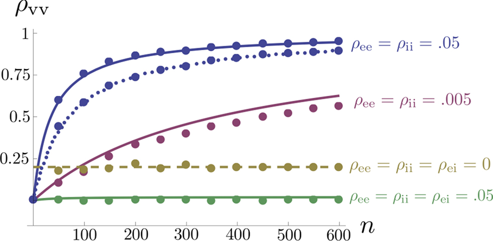
Figure 5. The effects of pooling on correlations between postsynaptic membrane potentials. Results of the linear approximation (solid, dotted, and dashed lines) match simulations (points). For the solid blue line, ρee = ρii = 0.05, and ρei = pe = pi = qe = qi = 0. The total number of excitatory and inhibitory inputs to each cell was n = ne + qene, and ni + qini respectively. Here ni = ne/3, with other parameters given in the Section “Materials and Methods.” The dotted blue line was obtained by including independent inputs, qe = qi = 1. The pink line was obtained by decreasing input correlations to ρee = ρii = 0.005. The solid green line was obtained by including excitatory–inhibitory correlations, ρei = 0.05, so that total input correlations canceled. The dashed tan line was obtained by setting ρee = ρii = ρei = qe = qi = 0 and pe = pi = 0.2 so that correlations are due to input overlap alone. In all cases, and  ℐ = 4ℰ. Standard errors are smaller than twice the radii of the points.
ℐ = 4ℰ. Standard errors are smaller than twice the radii of the points.The correlation between the membrane potentials has positive contributions from the correlation between the excitatory inputs  and between the inhibitory inputs
  Contributions coming from excitatory–inhibitory correlations (
 and
and  ) are negative, and can thus decorrelate the activity of downstream cells. This “cancellation” of correlations is observed in Figures 1
D and 5
, and can lead to asynchrony in recurrent networks (Hertz, 2010
; Renart et al., 2010
).
) are negative, and can thus decorrelate the activity of downstream cells. This “cancellation” of correlations is observed in Figures 1
D and 5
, and can lead to asynchrony in recurrent networks (Hertz, 2010
; Renart et al., 2010
).
and between the inhibitory inputs Contributions coming from excitatory–inhibitory correlations ( and ) are negative, and can thus decorrelate the activity of downstream cells. This “cancellation” of correlations is observed in Figures 1
D and 5
, and can lead to asynchrony in recurrent networks (Hertz, 2010
; Renart et al., 2010
).Implications for Synchronization in Feedforward Chains
Feedforward chains, like that depicted in Figure 6
A, have been studied extensively (Diesmann et al., 1999
; van Rossum et al., 2002
; Litvak et al., 2003
; Reyes, 2003
; Tetzlaff et al., 2003
; Câteau and Reyes, 2006
; Doiron et al., 2006
; Kumar et al., 2008
). In such networks, cells in a layer necessarily share some of their inputs, leading to correlations in their spiking activity (Shadlen and Newsome, 1998
). Frequently, spiking in deeper layers is highly synchronous (Reyes, 2003
; Tetzlaff et al., 2003
). However, in the presence of background noise, correlations can remain negligible (van Rossum et al., 2002
; Vogels and Abbott, 2005
).
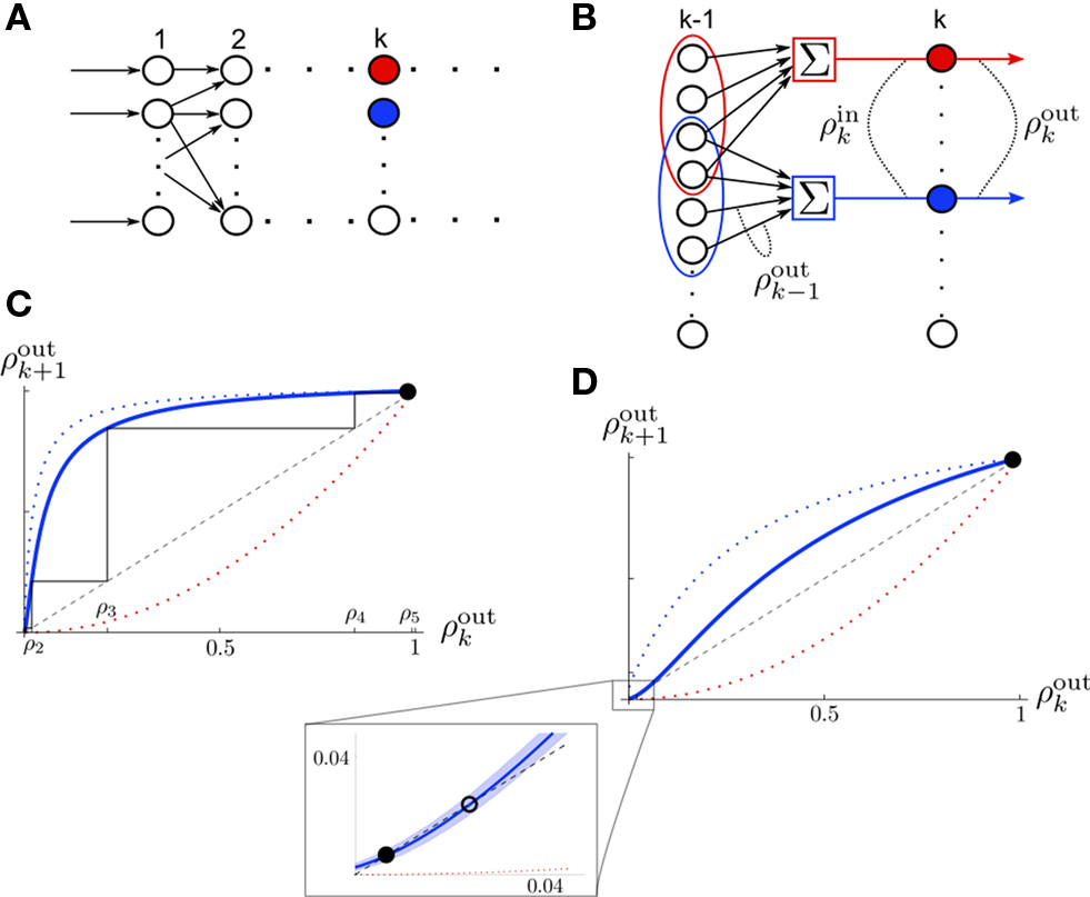
Figure 6. The development of synchrony in a feedforward chain can be understood using a model dynamical system (Tetzlaff et al. , 2003
). (A) Schematic diagram of the network. Each layer consists of Ne excitatory and Ni inhibitory cells. Each cell in layer k receives precisely ne excitatory and ni inhibitory, randomly selected inputs from layer k − 1. (B) Stages of processing in the feedforward network. Inputs from layer k − 1 are pooled with overlap, and drive the cells in layer k. (C) The correlation transfer map described by the pooling function, P(ρ) (blue dotted line), is composed with the decorrelating transfer function, S(ρ) = ρ2 (red dotted line), to obtain the mapping, T = S◦P (solid blue line). Cobwebs show the development of correlations in the discrete dynamical system defined by  with ρ0 = 0. Nearly perfect correlations develop by the fifth layer. The identity is shown as a dashed line. (D) Closer to balance (β≈1), the correlating effects of pooling are weakened, and the model develops a stable fixed point close to ρ = 0. However, cells may no longer decorrelate their inputs in the balanced regime, and fluctuations in the input statistics due to random connectivity can destabilize the fixed point and lead to synchrony. The shaded region in the inset represents the region two standard deviations away from the mean (blue line) when randomness in the overlap is taken into account (see Appendix). The standard deviations were calculated using Monte Carlo simulations. In C and D, Ne = 12000 and ne = 600. In C, Ni = 8000 and ni = 400. In D, Ni = 10500 and ni = 525 to obtain approximate balance (β = 600/525). Filled black circles represent stable fixed points and open black circles represent unstable fixed points.
with ρ0 = 0. Nearly perfect correlations develop by the fifth layer. The identity is shown as a dashed line. (D) Closer to balance (β≈1), the correlating effects of pooling are weakened, and the model develops a stable fixed point close to ρ = 0. However, cells may no longer decorrelate their inputs in the balanced regime, and fluctuations in the input statistics due to random connectivity can destabilize the fixed point and lead to synchrony. The shaded region in the inset represents the region two standard deviations away from the mean (blue line) when randomness in the overlap is taken into account (see Appendix). The standard deviations were calculated using Monte Carlo simulations. In C and D, Ne = 12000 and ne = 600. In C, Ni = 8000 and ni = 400. In D, Ni = 10500 and ni = 525 to obtain approximate balance (β = 600/525). Filled black circles represent stable fixed points and open black circles represent unstable fixed points.Feedforward chains amplify correlations as follows: When inputs to the network are independent, small correlations are introduced in the second layer by overlapping inputs. The inputs to each subsequent layer are pooled from the previous layer. The amplification of correlations by pooling is the primary mechanism for the development of synchrony (Compare solid and dotted blue lines in Figure 4
A). Overlapping inputs serve primarily to “seed” synchrony in early layers. The internal dynamics of the neurons and background noise can decorrelate the output of a layer, and compete with the correlation amplification due to pooling.
We develop this explanation by considering a feedforward network with each layer containing Ne excitatory and Ni inhibitory cells. Each cell in layer k + 1 receives ne excitatory and ni inhibitory inputs selected randomly from layer k. For simplicity we assume that all excitatory and inhibitory cells are dynamically identical and ℰ|VE − VL| = ℐ|VE − VL|. Spike trains driving the first layer are statistically homogeneous with pairwise correlations ρ0.
To explain the development of correlations, we consider a simplified model of correlation propagation (See also Renart et al., 2010
for a recurrent version). In the model, any two cells in a layer share the expected proportion pe = ne/Ne of their excitatory inputs and pi = ni/Ni of their inhibitory inputs (the expected proportions are taken with respect to random connectivity). We also assume that inputs are statistically identical across a layer.
For a pair of cells in layer k ≥ 1, let  and
and  represent the correlation coefficient between the total input currents and output spike trains respectively. The outputs from layer k are pooled (with overlap) to obtain the inputs to layer k + 1. Using the results developed above,
  and
and  for k ≥ 1, where (see Appendix and Tetzlaff et al., 2003
for a similar derivation)
for k ≥ 1, where (see Appendix and Tetzlaff et al., 2003
for a similar derivation)
and represent the correlation coefficient between the total input currents and output spike trains respectively. The outputs from layer k are pooled (with overlap) to obtain the inputs to layer k + 1. Using the results developed above, and for k ≥ 1, where (see Appendix and Tetzlaff et al., 2003
for a similar derivation)
Here β measures the balance between excitation and inhibition (see Materials and Methods). From our assumptions, β = ne/ni. With imbalance (β ≠ 1) and a large number of cells in a layer, pooling amplifies small correlations, P(ρ) > ρ, as discussed earlier.
To complete the description of correlation transfer from layer to layer, we relate the correlations between inputs to a pair of cells,  to correlations in their output spike trains,
  We assume that there is a transfer function, S, so that
  at each layer k. We additionally assume that S(0) = 0 and S(1) = 1, that is uncorrelated (perfectly correlated) inputs result in uncorrelated (perfectly correlated) outputs. We also assume that the cells are decorrelating, |ρ| > |S(ρ)| > 0 for ρ ≠ 0,1 (Shea-Brown et al., 2008
). This is an idealized model of correlation transfer, as output correlations depend on cell dynamics and higher order statistics of the inputs (Moreno-Bote and Parga, 2006
; de la Rocha et al., 2007
; Barreiro et al., 2009
; Ostojić et al., 2009
).
at each layer k. We additionally assume that S(0) = 0 and S(1) = 1, that is uncorrelated (perfectly correlated) inputs result in uncorrelated (perfectly correlated) outputs. We also assume that the cells are decorrelating, |ρ| > |S(ρ)| > 0 for ρ ≠ 0,1 (Shea-Brown et al., 2008
). This is an idealized model of correlation transfer, as output correlations depend on cell dynamics and higher order statistics of the inputs (Moreno-Bote and Parga, 2006
; de la Rocha et al., 2007
; Barreiro et al., 2009
; Ostojić et al., 2009
).
to correlations in their output spike trains, We assume that there is a transfer function, S, so that at each layer k. We additionally assume that S(0) = 0 and S(1) = 1, that is uncorrelated (perfectly correlated) inputs result in uncorrelated (perfectly correlated) outputs. We also assume that the cells are decorrelating, |ρ| > |S(ρ)| > 0 for ρ ≠ 0,1 (Shea-Brown et al., 2008
). This is an idealized model of correlation transfer, as output correlations depend on cell dynamics and higher order statistics of the inputs (Moreno-Bote and Parga, 2006
; de la Rocha et al., 2007
; Barreiro et al., 2009
; Ostojić et al., 2009
).Correlations between the spiking activity of cells in layers k + 1 are related to correlations in layer k by the layer-to-layer transfer function, T = S ○ P. The development of correlations across layers is modeled by the dynamical system,  with
with 
with When the network is not balanced (β ≠ 1), pooling amplifies correlations at each layer and the activity between cells in deeper layers can become highly correlated (see Figure 6
C). The output of the first layer is uncorrelated if the individual inputs are independent (ρ0 = 0). In this case all of the correlations between the total inputs to the second layer come from shared inputs,
These correlations are then reduced by the second layer of cells,  and subsequently amplified by pooling and input sharing before being received by layer 3,
  This process continues in subsequent layers. If the correlating effects of pooling and input sharing dominate the decorrelating effects of internal cell dynamics, correlations will increase from layer to layer (see Figure 6
C).
This process continues in subsequent layers. If the correlating effects of pooling and input sharing dominate the decorrelating effects of internal cell dynamics, correlations will increase from layer to layer (see Figure 6
C).
and subsequently amplified by pooling and input sharing before being received by layer 3, This process continues in subsequent layers. If the correlating effects of pooling and input sharing dominate the decorrelating effects of internal cell dynamics, correlations will increase from layer to layer (see Figure 6
C).When ρ0 = 0, overlapping inputs increase the input correlation to layer 2, but have a negligible effect on the mapping once correlations have developed since the effects of pooling dominate [see Eq. (14) and the dashed blue line in Figure 4
A which shows that the effects of input overlaps are small when ne is large, ρ > 0 and β ≠ 1]. Therefore, shared inputs seed correlated activity at the first layer, and pooling drives the development of larger correlations. When ρ0 = 0, we cannot expect large correlations before layer 3, but when ρ0 > 0 large correlations can develop by layer 2.
To verify this conclusion, we constructed a two-layer feedforward network with no overlap between inputs (Pe = Pi = 0). In Figure 7
A, the inputs to layer 1 were independent (ρ0 = 0), and the firing of cells in layer 2 was uncorrelated. In Figure 7
B, we introduced small correlations (ρ0 = 0.05) between inputs to layer 1. These correlations were amplified by pooling so that strong synchrony is observed between cells in layer 2. We compared these results with a standard feedforward network with overlap in cell inputs (Figure 7
C, where Pe = Pi = 0.05). Inputs to layer 1 were independent (ρ0 = 0), and hence outputs from layer 1 uncorrelated. Dependencies between inputs to layer 2 were weak and due to overlap alone,  Cells in layer 3 received pooled inputs from layer 2, and their output was highly correlated.
Cells in layer 3 received pooled inputs from layer 2, and their output was highly correlated.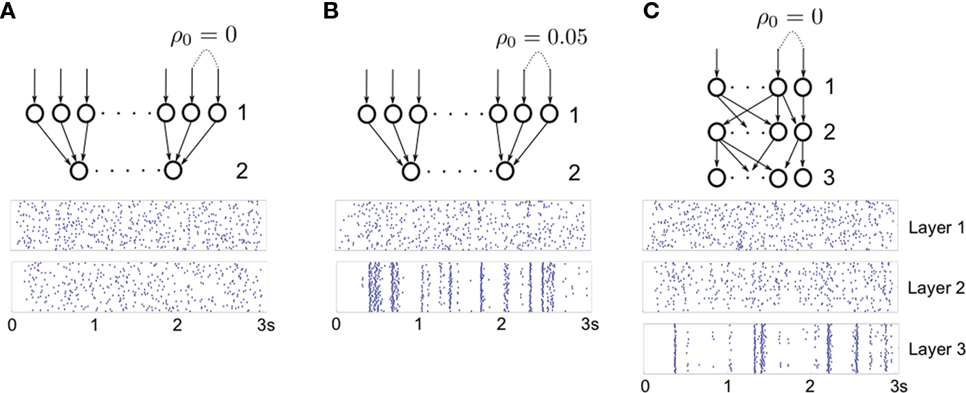
Figure 7. Development of synchrony in feedforward networks. (A) A feedforward network with no overlap and independent, Poisson input. For excitatory cells, we set ℰ ≈ 1.55nS·ms, and ℐ ≈ 4.67nS·ms. For inhibitory cells, ℰ ≈ 3.61nS·ms, and ℐ ≈ 10.82nS·ms. (B) Same as A, except inputs to layer 1 are correlated with coefficient ρ0 = 0.05. The network is highly synchronized in the second layer, even though inputs do not overlap. (C) Same as A, except for the presence of overlapping inputs (pe = pi = 0.05). Correlations due to overlap in the input to layer 2 result in average correlations of 0.05 between input currents. Layer 3 cells in C synchronize (Compare with layer 2 in B). In all three figures, each cell in the first layer was driven by excitatory Poisson inputs with rate ν0 = 100 Hz.
These results predict that correlations between spike trains develop in deeper layers, but they do not not directly address the timescale of the correlated behavior. In simulations, spiking becomes tightly synchronized in deeper layers (see for instance Litvak et al., 2003
; Reyes, 2003
; and Figure 7
). This can be understood using results in Maršálek et al. (1997) and Diesmann et al. (1999)
where it is shown that the response of cells to volleys of spikes is tighter than the volley itself. The firing of individual cells in the network becomes bursty in deeper layers and large correlations are manifested in tightly synchronized spiking events. Alternatively, one can predict the emergence of synchrony by observing that pooling increases correlations over finite time windows (see next section and Appendix) and therefore the analysis developed above can be adapted to correlations over small windows.
Balanced feedforward networks
In the simplified feedforward model above, when excitation balances inhibition, that is β ≈ 1, correlations between the pooled inputs to a layer are due to overlap alone,  for all k. The correlating effects of this map are weak, and this would seem to imply that cells in balanced feedforward chains remain asynchronous. Indeed, our model of correlation propagation displays a stable fixed point at low values of ρ when β ≈ 1 (see Figure 6
D). However, in practice, synchrony is difficult to avoid without careful fine-tuning (Tetzlaff et al., 2003
), and almost always develops in feedforward chains (Litvak et al., 2003
). We provide some reasons for this discrepancy.
for all k. The correlating effects of this map are weak, and this would seem to imply that cells in balanced feedforward chains remain asynchronous. Indeed, our model of correlation propagation displays a stable fixed point at low values of ρ when β ≈ 1 (see Figure 6
D). However, in practice, synchrony is difficult to avoid without careful fine-tuning (Tetzlaff et al., 2003
), and almost always develops in feedforward chains (Litvak et al., 2003
). We provide some reasons for this discrepancy.Our focus so far has been on correlations over infinitely large time windows (see Materials and Methods where we define ρxy). Even when the membrane potentials are nearly uncorrelated over large time windows, differences between the excitatory and inhibitory synaptic time constants can cause larger correlations over smaller time windows (Renart et al., 2010
). This can, in turn, lead to significant correlations between the output spike trains. We discuss this effect further in the Appendix and give an example in Figure 8
. In this example, the correlations between the membrane potentials over long windows are nearly zero due to cancellation (see Figure 8
A where ρVV = 0.0174 ± 0.0024 s.e. with threshold present), but positive over shorter timescales. The cross-covariance function between the output spike trains is primarily positive, yielding significant spike train correlations (ρspikes = 0.1570 ± 0.0033 s.e.). Therefore, the assumption that pairs of cells decorrelate their inputs may not be valid in the balanced case.
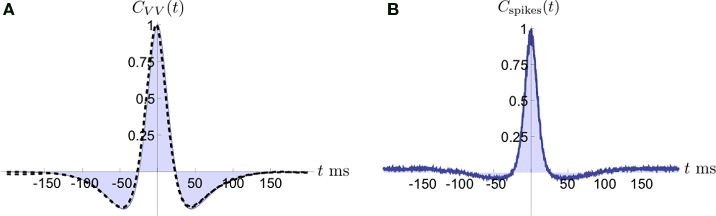
Figure 8. Cross-covariance functions between membrane potentials and output spike trains. (A) The cross-covariance function between membrane potentials, scaled so that its maximum is 1. The linear approximation in Eq. (16) (blue, shaded) agrees with simulations of the full conductance-based model (black dashed line). Differences between simulations with and without threshold are too small to be observable (8000 simulations 10s each; simulations with and without threshold are shown). Parameters are as in Figure 1
D. The cells are balanced with ρee = ρii = ρei = 0.05 so that the correlation between the membrane potentials over long time windows is essentially zero (ρvv = 0.0085 ± 0.0024 s.e. unthresholded, and ρvv = 0.0174 ± 0.0024 s.e. thresholded). However, correlations over shorter time windows are positive as indicated by the central peak in the cross-covariance function. (B) The cross-covariance between the output spike trains is mostly positive. The correlation between the output spike trains was ρspikes = 0.1570 ± 0.0033 s.e. (500 simulations of 100s each with same parameters as in A.
Another source of discrepancies between the idealized model and simulations of feedforward networks are inhomogeneities, which become important when balance is exact. Note that Eq. (14) is an approximation obtained by ignoring fluctuations in connectivity from layer to layer. In a random network, inhomogeneities will be introduced by variability in input population overlaps. To fully describe the development of correlations in a feedforward network, it is necessary to include such fluctuations in a model of correlation propagation. The asynchronous fixed point that appears in the balanced case has a small basin of attraction and fluctuations induced by input inhomogeneities could destroy its stability (see Figure 6
D). Other sources of heterogeneity can further destabilize the asynchronous state (see Appendix).
It has been shown that asynchronous states can be stabilized through the decorrelating effects of background noise (van Rossum et al., 2002
; Vogels and Abbott, 2005
). To emulate these effects, a third transfer function, N, can be added to our model. The correlation transfer map then becomes T(ρ) = S◦N◦P(ρ). Sufficiently strong background noise can increase decorrelation from input to output of a layer, and stabilize the asynchronous fixed point.
We have illustrated how pooling and shared inputs can impact correlations between the inputs and free membrane voltages of postsynaptic cells in a feedforward setting. The increase in correlation due to pooling was discussed in a simpler setting in (Bedenbaugh and Gerstein, 1997
; Super and Roelfsema, 2005
; Chen et al., 2006
; Stark et al., 2008
), and similar ideas were also developed for the variance alone in (Salinas and Sejnowski, 2000
; Moreno-Bote et al., 2008
). The saturation of the signal-to-noise ratio with increasing population size observed in (Zohary et al., 1994
) has a similar origin. Our aim was to present a unified discussion of these results, with several generalizations.
Other mechanisms, such as recurrent connectivity between cells receiving the inputs, can modulate correlated activity (Schneider et al., 2006
; Ostojić et al., 2009
). Importantly, the cancellation of correlations may be a dynamic phenomenon in recurrent networks, as observed in (Hertz, 2010
; Renart et al., 2010
). On the other hand, neurons may become entrained to network oscillations, resulting in more synchronous firing (Womelsdorf et al., 2007
). A full understanding of the statistics of population activity in neuronal networks will require an understanding of how these mechanisms interact to shape the spatiotemporal properties of the neural response.
The results we presented relied on the assumption of linearity at the different levels of input integration. These assumptions can be expected to hold at least approximately. For instance, there is evidence that membrane conductances are tuned to produce a linear response in the subthreshold regime (Morel and Levy, 2009
). The assumptions we make are likely to break down at the level of single dendrites where nonlinear effects may be much stronger (Johnston and Narayanan, 2008
). The effects of correlated inputs to a single dendritic branch deserve further theoretical study (Gasparini and Magee, 2006
; Li and Ascoli, 2006
).
We demonstrated that the structure of correlations in a population may be difficult to infer from pooled activity. For instance, a change in pairwise correlations between individual cells in two populations causes a much smaller change in the correlation between the pooled signals. With a large number of inputs, the change in correlations between the pooled signals might not be detectable even when the change in the pairwise correlations is significant.
While we discussed the growth of second order correlations only, higher order correlations also saturate with increasing population size. For example, in a 3-variable generalization of the homogeneous model from Figure 3
A, it can be shown that  where ne is the size of each population and
  is the triple correlation coefficient (Stratonovich, 1963
) between the pooled signals E1, E2, and E3. The reason that higher order correlations also saturate follows from the generalization of the following observation at second order: Pooling amplifies correlations because the variance and covariance grow asymptotically with the same rate in ne. In particular
is the triple correlation coefficient (Stratonovich, 1963
) between the pooled signals E1, E2, and E3. The reason that higher order correlations also saturate follows from the generalization of the following observation at second order: Pooling amplifies correlations because the variance and covariance grow asymptotically with the same rate in ne. In particular  and
and  both behave asymptotically like
  and their ratio,
  approaches unity (Bedenbaugh and Gerstein, 1997
; Salinas and Sejnowski, 2000
; Moreno-Bote et al., 2008
).
approaches unity (Bedenbaugh and Gerstein, 1997
; Salinas and Sejnowski, 2000
; Moreno-Bote et al., 2008
).
where ne is the size of each population and is the triple correlation coefficient (Stratonovich, 1963
) between the pooled signals E1, E2, and E3. The reason that higher order correlations also saturate follows from the generalization of the following observation at second order: Pooling amplifies correlations because the variance and covariance grow asymptotically with the same rate in ne. In particular and both behave asymptotically like and their ratio, approaches unity (Bedenbaugh and Gerstein, 1997
; Salinas and Sejnowski, 2000
; Moreno-Bote et al., 2008
).We concentrated on correlations over infinitely long time windows (see Materials and Methods where we define ρxy). However, pooling amplifies correlations over finite time windows in exactly the same way as correlations over large time windows. Due to the filtering properties of the cells, the timescale of correlations between downstream membrane potentials may not reflect that of the inputs. We discuss this further in the Appendix where the auto- and cross-covariance functions between the membrane potentials are derived.
To simplify the presentation, we have so far assumed stationary. However, since Eq. (2) applies to the Pearson correlation between any pooled data, all of the results on pooling can easily be extended to the non-stationary case. In the non-stationary setting, the cross-covariance function has the form Rxy(s, t) = cov (x(s), y(s + t)), but there is no natural generalization of the asymptotic statistics defined in Eq. (1).
Correlated neural activity has been observed in a variety of neural populations (Gawne and Richmond, 1993
; Zohary et al., 1994
; Vaadia et al., 1995
), and has been implicated in the propagation and processing of information (Oram et al., 1998
; Maynard et al., 1999
; Romo et al., 2003
; Tiesinga et al., 2004
; Womelsdorf et al., 2007
; Stark et al., 2008
), and attention (Steinmetz et al., 2000
; Mitchell et al., 2009
). However, correlations can also introduce redundancy and decrease the efficiency with which networks of neurons represent information (Zohary et al., 1994
; Gutnisky and Dragoi, 2008
; Goard and Dan, 2009
). Since the joint response of cells and recorded signals can reflect the activity of large neuronal populations, it will be important to understand the effects of pooling to understand the neural code (Chen et al., 2006
).
Derivation of Eq. (10)
Equation (10) can be derived from Eq. (2). However, we find that it is more easily derived directly. We will calculate the variance,  and covariance
  between the pooled signals.
and covariance between the pooled signals.The covariance is given by the sum of all pairwise covariances between the populations,  Each cell receives
  inputs so that there are (ne + qene)2 terms that appear in this sum. However, the qene “independent” inputs from each pool are uncorrelated with all other inputs and therefore don’t contribute to the sum. Of the remaining
  pairs, nepe are shared and therefore have correlation
  These shared processes therefore collectively contribute
  to
to  The remaining
  processes are correlated with coefficient ρee and collectively contribute
  The pooled covariance is thus
Each cell receives inputs so that there are (ne + qene)2 terms that appear in this sum. However, the qene “independent” inputs from each pool are uncorrelated with all other inputs and therefore don’t contribute to the sum. Of the remaining pairs, nepe are shared and therefore have correlation These shared processes therefore collectively contribute to The remaining processes are correlated with coefficient ρee and collectively contribute The pooled covariance is thus
The variance is given by the sum of all pairwise covariances within a population,  As above, there are ne + qene neurons in the population, so that the sum has (ne + qene)2 terms. Of these, ne + qene are “diagonal” terms (e1 = e2), each contributing
  for a total contribution of
  to
to  The processes from the independent pool do not contribute any additional terms. This leaves ne(ne − 1) correlated pairs which each contribute
  for a collective contribution of
  giving
As above, there are ne + qene neurons in the population, so that the sum has (ne + qene)2 terms. Of these, ne + qene are “diagonal” terms (e1 = e2), each contributing for a total contribution of to The processes from the independent pool do not contribute any additional terms. This leaves ne(ne − 1) correlated pairs which each contribute for a collective contribution of giving
Now,  can be simplified to give Eq. (10). Equations for
  and
and  can be derived identically.
can be simplified to give Eq. (10). Equations for and can be derived identically.Finite-Time Correlations and Cross-Covariances
Throughout the text, we concentrated on correlations over large time windows. However, the effects of pooling described by Eq. (2) apply to the correlation, ρxy(t), between spike counts over any time window of size t, defined by  where
where  is the spike count over [0,t] for the spike train x(t). The equation also applies to the instantaneous correlation at time t, defined by
  Thus pooling increases correlations over all timescales equally.
where is the spike count over [0,t] for the spike train x(t). The equation also applies to the instantaneous correlation at time t, defined by Thus pooling increases correlations over all timescales equally.However, the cell filters the pooled inputs to obtain the membrane potentials and, as a result, the correlations between membrane potentials is “spread out” in time (Tetzlaff et al., 2008
). To quantify this effect, we derive an approximation to the auto- and cross-covariance functions between the membrane potentials.
The pooled input spike trains are obtained from from a weighted sum of the individual excitatory and inhibitory spike trains (see Materials and Methods). As a result cross-covariance functions between the pooled spike trains are just sums of the individual cross-covariance functions,  for X, Y = E1, E2, I1, I2 and x, y = e, i accordingly. Thus only the magnitude of the cross-covariance functions is affected by pooling. The change in magnitude is quadratic in ne or ni. This is consistent with the observation that pooling amplifies correlations equally over all timescales.
for X, Y = E1, E2, I1, I2 and x, y = e, i accordingly. Thus only the magnitude of the cross-covariance functions is affected by pooling. The change in magnitude is quadratic in ne or ni. This is consistent with the observation that pooling amplifies correlations equally over all timescales.The conductances are obtained by convolving the total inputs with the synaptic filter kernels,

The cross-covariance between the conductances can therefore be written as a convolution of the cross-covariance function between the input signals and the deterministic cross-covariance between the synaptic kernels (Tetzlaff et al., 2008
). In particular,

for X, Y = E1, E2, I1, I2 and x, y = e, i accordingly, where  is the deterministic cross-covariance between the synaptic filters, αx and αy. Note that total correlations remain unchanged by convolution of the input spike trains with the synaptic filters, since the integral of a convolution will be equal to the product of the integrals (Tetzlaff et al., 2008
).
is the deterministic cross-covariance between the synaptic filters, αx and αy. Note that total correlations remain unchanged by convolution of the input spike trains with the synaptic filters, since the integral of a convolution will be equal to the product of the integrals (Tetzlaff et al., 2008
).The total input currents, JK(t) = – (VL–VI))/Cm, obtained from the linearization of the conductance-based model described in the Section “Materials and Methods” are simply linear combinations of the individual conductances. The cross-covariance function between the input currents is therefore a linear combination of those between the conductances,
(VL–VI))/Cm, obtained from the linearization of the conductance-based model described in the Section “Materials and Methods” are simply linear combinations of the individual conductances. The cross-covariance function between the input currents is therefore a linear combination of those between the conductances,
Combining this result with Eq. (1), yields the correlation,  between the total input currents given in Eq. (13).
between the total input currents given in Eq. (13).Using the solution of the linearized equations described in the Section “Materials and Methods”, we obtain a linear approximation to the cross-covariance functions,

for h,k = 1,2 where  is the cross-covariance between the linear kernel, K, and itself. The convolution with (K*K)(t) scales the area of both the auto- and cross-covariance functions by a factor of
  and therefore leaves the ratio of the areas,
  unchanged. Thus, the linear approximation predicts that
is the cross-covariance between the linear kernel, K, and itself. The convolution with (K*K)(t) scales the area of both the auto- and cross-covariance functions by a factor of and therefore leaves the ratio of the areas, unchanged. Thus, the linear approximation predicts that When the total inputs are strong, τeff is small and we can simplify Eq. (16) by approximating (K*K)(t) with a delta function with mass  so that
  and similarly for
  This approximation is valid when the synaptic time constants are significantly larger than τeff, which is likely to hold in high conductance states. We compare this approximation to cross-covariance functions obtained from simulations in Figure 8
.
This approximation is valid when the synaptic time constants are significantly larger than τeff, which is likely to hold in high conductance states. We compare this approximation to cross-covariance functions obtained from simulations in Figure 8
.
so that and similarly for This approximation is valid when the synaptic time constants are significantly larger than τeff, which is likely to hold in high conductance states. We compare this approximation to cross-covariance functions obtained from simulations in Figure 8
.In all examples considered, the cross-covariance functions have exponentially decaying tails. We define the correlation time constant,  as a measure of the decay rate of the exponential tail. If t ≫ τxy, then x(s) and y(s + t) can be regarded as approximately uncorrelated and
  (Stratonovich, 1963
).
(Stratonovich, 1963
).
as a measure of the decay rate of the exponential tail. If t ≫ τxy, then x(s) and y(s + t) can be regarded as approximately uncorrelated and (Stratonovich, 1963
).The time constant of a convolution between two exponentially decaying functions is just the maximum time constant of the two functions. Thus, from the results above, the correlation time constant between the membrane potentials is the maximum of the correlation time constants between the inputs, the synaptic time constants, and the effective membrane time constant  where
where 

 and
and  are the time constants of the input spike trains and τe and τi are synaptic time constants. Thus the cross-covariances functions between the membrane potentials are generally broader than the cross-covariance functions between the spike train inputs.
where and are the time constants of the input spike trains and τe and τi are synaptic time constants. Thus the cross-covariances functions between the membrane potentials are generally broader than the cross-covariance functions between the spike train inputs.Derivation of Eq. (14)
Consider a feedforward network where each layer consists of Ne excitatory cells and Ni inhibitory cells; each cell in layer k receives ne excitatory and ni inhibitory inputs from layer (k − 1), and these connections are chosen randomly and independently across neurons in layer k. Then the degree of overlap in the excitatory and inhibitory inputs to a pair of cells in layer k is a random variable. Following the derivation in Derivation of Eq. (10) in Appendix,
where se denotes the number of common excitatory inputs between the two cells. To understand the origin of se, suppose the ne excitatory inputs to cell 1 have been selected. Then the selection of the ne excitatory inputs to cell 2 involves choosing, without replacement, from two pools: the first, of size ne, projects to cell 1, and the second, of size (Ne − ne), does not. Therefore, se is follows a hyper-geometric distribution with parameters (Ne, ne, ne), and has mean  In addition, this random variable is independently selected amongst each pair in layer k. Using the mean value of se, we obtain Eq. (10).
In addition, this random variable is independently selected amongst each pair in layer k. Using the mean value of se, we obtain Eq. (10).For simplicity, we assume that ℰ|VE − VL| = ℐ |VI − VL|, so that β = ni/ne. If we assume that the statistics in the (k − 1)st layer are uniform across all cells and cell types (i.e.,  and σe = σi) then by substituting Eq. (10) and the equivalent forms for ρII, ρEI in to Eq. (13), we may write the input correlations to the kth layer as
and σe = σi) then by substituting Eq. (10) and the equivalent forms for ρII, ρEI in to Eq. (13), we may write the input correlations to the kth layer as
Substituting the values of the covariances and variances, and dividing the numerator and denominator by (ℰ|VE − VL|σe)2, we get
Rearranging terms and dividing numerator and denominator by  along with the substitution β = ne/ni, we have
along with the substitution β = ne/ni, we have
This equation takes into account the variations in overlap due to finite size effects since se and si are random variables. Eq. (14) in the text represents the expected value P(ρ) = 〈ρin〉 which can be obtained by replacing the variables se and si in Eq. (17) with their respective means, 〈se〉 = nepe and 〈si〉 = nipi. The expectation above is taken over realizations of the random connectivity of the feedforward network.
To calculate the standard deviation for the inset in Figure 6
D, we ran Monte Carlo simulations, drawing se and si from a hypergeometric distribution and calculating the resulting transfer,  using Eq. (17). Note, however, that Eq. (17) and the inset in Figure 6
D, do not account for all of the effects of randomness which may destabilize the balanced network. In deriving Eq. (17), we assumed that the statistics in the second layer were uniform. However, variations in the degree of overlap in one layer will cause inhomogeneities in the variances and rates at the next layer. In a feedforward setting, these inhomogeneities are compounded at each layer to destabilize the asynchronous fixed point.
using Eq. (17). Note, however, that Eq. (17) and the inset in Figure 6
D, do not account for all of the effects of randomness which may destabilize the balanced network. In deriving Eq. (17), we assumed that the statistics in the second layer were uniform. However, variations in the degree of overlap in one layer will cause inhomogeneities in the variances and rates at the next layer. In a feedforward setting, these inhomogeneities are compounded at each layer to destabilize the asynchronous fixed point.Definitions and Values of Variables Used in the Text
The authors declare that the research was conducted in the absence of any commercial or financial relationships that could be construed as a potential conflict of interest.
We thank Jaime de la Rocha, Brent Doiron and Eric Shea-Brown for helpful discussions. We also thank the reviewers and the handling editor for numerous useful suggestions. This work was supported by NSF Grants DMS-0604429 and DMS-0817649 and a Texas ARP/ATP award.
Super, H., and Roelfsema, P. (2005). Chronic Multiunit Recordings in Behaving Animals: Advantages and Limitations. Development, dynamics and pathology of neuronal networks: from molecules to functional circuits: proceedings of the 23rd International Summer School of Brain Research, held at the Royal Netherlands Academy of Arts and Sciences, Amsterdam, from 25–29 August 2003, 263.