Higher-order correlations in non-stationary parallel spike trains: statistical modeling and inference

Introduction

It has long been suggested that fundamental insight into the nature of neuronal computation requires the understanding of the cooperative dynamics of populations of neurons (Hebb, 1949 ). A controversial issue in this debate is the role of correlations among nerve cells. On the one hand, an increasing body of both experimental (e.g., Gray and Singer, 1989 ; Vaadia et al., 1995 ; Riehle et al., 1997 ; Bair et al., 2001 ; Kohn and Smith, 2005 ; Shlens et al., 2006 ; Fujisawa et al., 2008 ; Pillow et al., 2008 ) and theoretical (Abeles, 1991 ; Diesmann et al., 1999 ; Kuhn et al., 2003 ) literature supports the concept of cooperative computation on various temporal and spatial scales. On the other hand, the mostly detrimental effect of correlations on rate-based information transmission and processing (Abbott and Dayan, 1999 ; Averbeck and Lee, 2006 ; Josić et al., 2009 ) has generated a strong opposition toward correlation-based concepts of cortical coding (Shadlen and Newsome, 1998 ; Averbeck et al., 2006 ; Schneidman et al., 2006 ; Ecker et al., 2010 ). Evidently, a thorough description of the correlation structure of neuronal populations is an indispensable prerequisite to resolve these opposing theoretical viewpoints (Brown et al., 2004 ).

Experimental reports on coordinated activity at the level of spike trains resort almost exclusively to correlations between pairs of nerve cells (e.g., Eggermont, 1990 ; Vaadia et al., 1995 ; Kreiter and Singer, 1996 ; Riehle et al., 1997 ; Kohn and Smith, 2005 ; Sakurai and Takahashi, 2006 ; Fujisawa et al., 2008 ; Ecker et al., 2010 ). Such pairwise correlations cannot, as a matter of principle, resolve the cooperative activity of neuronal populations to the extent required for rigorous hypothesis testing (Gerstein et al., 1989 ; Martignon et al., 2000 ; Brown et al., 2004 ). In particular, whether or not coincident spikes of pairs of neurons participate in synchronized “cluster-events” cannot be decided on measurements of pairwise correlation alone; this can only be achieved by the systematic assessment of higher-order correlations, i.e., statistical couplings among triplets, quadruplets, and larger groups (Martignon et al., 1995 ; Staude et al., 2010 ). Importantly, the nonlinear dynamics of spike generation makes neurons extremely sensitive for synchrony in their input pools (Softky, 1995 ; König et al., 1996 ). Ignoring these higher-order correlations in the statistical description of spiking populations is therefore hardly advisable (Bohte et al., 2000 ; Kuhn et al., 2003 ).

Initially, the main obstacle for assessing the higher-order structure of neuronal populations were limitations in experimental methodology, as until recently state-of-the-art electrophysiological setups allowed to record only few neurons simultaneously. The advent of multi-electrode arrays and optical imaging techniques, however, now reveals fundamental shortcomings of available analysis tools (Brown et al., 2004 ). Mathematical frameworks to model and estimate higher-order correlations typically assign one “interaction parameter” for every subgroup of the population, leading to a 2^N − 1 dimensional model for a population comprising N neurons (Martignon et al., 1995 , 2000 ). The associated estimation problem greatly suffers from this combinatorial explosion: the number of parameters to be estimated from the available sample size (a population of N = 100 neurons implies ∼10³⁰ parameters while 100 s of data provide only ∼10⁶ samples) illustrates the principal infeasibility of this approach. In fact, the estimation of such higher-order correlations runs into severe practical problems even for populations of N ∼ 10 neurons (Martignon et al., 1995 , 2000 ; Del Prete et al., 2004 ; Shlens et al., 2006 ; Montani et al., 2009 ). The severeness of this limitation is further underscored by the fact that the significance of higher-order correlations computed from small populations (N ∼ 10; Schneidman et al., 2006 ; Shlens et al., 2006 ) can generally not be extrapolated to large populations (Roudi et al., 2009 ). Taken together, while recent progress in experimental technique allows for the simultaneous recording of the spiking activity of tens to hundreds nerve cells, a faithful statistical description of the resulting activity that includes correlations of higher order is greatly hampered by the limitations of available data analysis techniques.

We have recently presented a novel method for a cumulant-based inference for the presence of higher-order correlations (CuBIC) that avoids the need for extensive sample sizes (Staude et al., 2007 , 2009 ). Instead of directly estimating correlation parameters from all subgroups, CuBIC aims only at population-average correlations, estimated via the cumulants of the pooled and discretely sampled spiking activity of all recorded neurons (population spike counts). The presence of higher-order correlations is then inferred from measured cumulants of low order by exploiting certain constraining relations among correlations of different orders in a statistical model of correlated spiking. CuBIC avoids the direct estimation of higher-order correlations, but decides whether or not lower order cumulants require the presence of higher-order correlations. Focusing on such less specific questions drastically reduces the requirements with respect to the sample size: when applied to artificial data, CuBIC reliably infers higher-order correlations from large (N ≳ 100), even weakly correlated populations (pairwise correlation coefficient c ∼ 0.01) that were generated with reasonable sample sizes (T < 100 s, Staude et al., 2009 ).

As a statistical model, CuBIC employs the compound Poisson process (CPP), where correlations are induced by the insertion of coincident events in continuous time, i.e., before binning is applied (Ehm et al., 2007 ; Johnson and Goodman, 2007 ; Brette, 2009 ; Staude et al., 2010 ). Interestingly, this model of correlation fits perfectly to measuring (higher-order) correlations via connected cumulants of the binned spike trains (Staude et al., 2010 ), a common framework for (higher-order) correlation measures. The simple relationship of the unknown model parameters, i.e., the orders of correlation present in the data, and the observable cumulants of the population spike count allows to devise null-hypotheses concerning the orders of correlation in the data (the details of the CPP and CuBIC are explained in Section “The Stationary Case”). Combining tests against different null-hypothesis yields a lower bound for the maximal order of correlation in the data.

A central assumption in the original presentation of CuBIC (Staude et al., 2009 ) was that the statistics of spiking in the population does not change over time (stationarity). As both experimental cues and/or internal processes often induce transients or fluctuations of firing rates, this central assumption is frequently violated in electrophysiological data.

In the present study, we describe a non-stationary version of the CPP by decoupling the correlation structure from the spike intensity of the population (see Section “The Non-stationary Case”). Using the “law of total cumulance” we are able to incorporate non-stationarities in firing rate into the computation of the cumulants of the population spike counts. These rate-adjusted cumulants are then used to adapt CuBIC to infer higher-order correlations also from non-stationary data. This adaptation requires a specification of the kind of non-stationarity in terms of a parametric family of distributions for the bin-wise mean firing rates (the “carrier distribution”). Allowing for uniform rate fluctuations, for instance, yields as a result that the data must have correlations of some minimal order even if firing rates fluctuated uniformly from bin to bin. In this sense, the choice of a family for the carrier distribution implies a demarcation line between “genuine” correlation and “artifacts” due to rate (co-)variation (Staude et al., 2008 ). Numerical simulations reveal that the adaptation corrects for false positive inference of correlations in data with pure rate co-variation, while allowing for potential variations in firing rates has a surprisingly small effect on CuBIC’s sensitivity for correlations (see Case Studies). Furthermore, we find that a perfect match between the true carrier family and the family allowed in the adapted CuBIC does not seem to be fundamentally important to guarantee reliable test performance.

The Stationary Case

Cumulants and the Compound Poisson Process

Population spike count

The basic observable of this study is the pattern vector X(s): = (X₁(s),…,X_N(s)), where X_i(s) is the discretized spike count of the ith neuron in the bin [sh,(s + 1)h) of width h (a complete list of symbols is provided in Section “List of Symbols” in Appendix). Given X(s), we define the population spike count Z(s) as the total number of spikes in the population in the sth bin (Figure 1 )

FIGURE 1

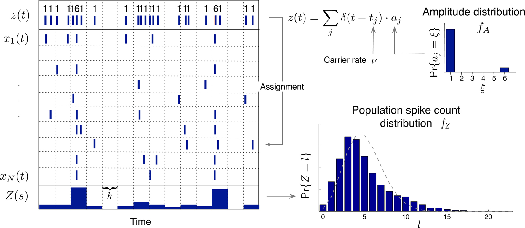
Figure 1. Schema of the compound Poisson process and its measurement. Left: spike event times (horizontal bars) of individual neurons x₁(t),…,x_N(t) and tick marks of the carrier process z(t) (top) with the associated amplitudes (numbers above the ticks). The population spike count Z(s) (below the spike trains) counts the number of spikes across all neurons in bins of width h (dotted lines). Right: distributions of the amplitudes a_j, f_A (top) and of the population spike counts, f_Z, (bottom; blue bars: f_Z from 100 s of data with the given amplitude distribution, estimated using a bin size of h = 5 ms; dashed line: Poisson fit, corresponding to an independent population with the same firing rates). To construct a population of correlated spike trains, amplitudes a_j are drawn for all events t_j in the carrier process i.i.d from f_A. Individual processes x_i(t) are constructed by assigning subsequent events of the carrier process z(t) into a_j “child” processes x_i(t) (here, events are assigned randomly to the specific process IDs). Correlations of order ξ are induced, whenever events in the carrier process are copied into more than ξ processes, i.e., if the amplitude distribution assigns non-zero probabilities for amplitudes ≥ ξ.

In the case where the X_i are binary (“1” for one or more spikes in the bin, “0” for no spike), Z(s) is simply the number of neurons that spike in the sth bin. As opposed to other frameworks for correlation analysis (e.g., Aertsen et al., 1989 ; Martignon et al., 1995 ; Grün et al., 2002a ; Nakahara and Amari, 2002 ; Shlens et al., 2006 ), however, the method presented in this study does not assume binary variables.

We here assume that Z(s) and Z(s + k) are independent for k ≠ 0 (zero memory). Furthermore, let us for now assume that the distribution of Z(s) does not depend on the time bin s (stationarity). This critical assumption will be relaxed in Section “The Non-stationary Case”.

Correlations and cumulants

In the present framework, correlations among the variables X_i are measured by mixed or “connected” cumulants. Like the more familiar (raw) moments E[Z^m] of a random variable Z, the univariate cumulants κ_m[Z] characterize the shape of its distribution (see, e.g., Stratonovich, 1967 ; Gardiner, 2003 ). For the first two cumulants, the expectation value and the variance, the latter can be expressed in terms of the former by the well-known expressions κ₁[Z] = E[Z] and κ₂[Z] = E[Z²] − E[Z]² = Var[Z]. Similar equalities for higher cumulants are exceedingly complicated, but algorithms for their computations are available (see Stuart and Ord, 1987 for explicit expressions for m ≤ 10, Section “Cumulants of the Non-stationary CPP” for a straightforward, and Di Nardo et al., 2008 for a more advanced algorithm). For notational consistency, we will from now on use the cumulant notation, e.g., use the terms “first/second cumulant” instead of the more familiar “mean/variance”.

Multivariate, or “connected”, cumulants arise when the variable under consideration is a sum of correlated variables. For m = 2 and , for instance, we have the well-known formula

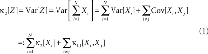
Hence, the second-order cumulant correlations Cov[X_i,X_j] = κ_1,1[X_i,X_j] measure the degree of additive linearity of κ₂[Z]. Higher-order cumulant correlations are generalizations of the covariance in exactly this sense, and mth order correlations arise when κ_m[Z] is decomposed into expressions involving the individual X_i. The following definition fixes the notation used in the remainder of this study, for a precise definition we refer to the literature (e.g., Stuart and Ord, 1987 ; Gardiner, 2003 ; Staude et al., 2009 ; for details on cumulant correlations see also Streitberg, 1990 ; Staude et al., 2010 ).

Definition 1 Let X = (X₁,…,X_N) be an N-dimensional random variable, e.g., the spike counts of N parallel spike trains, let M = {m₁,…,m_κ} be a subset of {1,…,N} of size k, and denote by σ(M) ∈ {0,1}^N the binary indicator vector of the set M, whose ith component is 1 if i ∈M and 0 otherwise. Then we measure kth order correlations among by the connected cumulant κ_σ(M)[X]. We say that X has correlations of order k if and only if at least one kth order connected cumulant of X is non-zero.

The following generalization of Eq. 1 is a straightforward consequence of the construction of connected cumulants (Staude et al., 2010 ).

Theorem 1 The mth cumulant κ_m[Z] of depends on the summed correlations among the X_i of all orders ≤m, but is independent of correlations of orders >m.

By the above theorem, κ_m[Z] is a measure for the total correlation in the population of all orders ≤m. While a correction of the second cumulant for the influence of the single process statistics would be straightforward (subtracting in Eq. 1, see Staude et al., 2009 ), correcting higher cumulants for the influence of correlations of lower order is exceedingly complicated. We therefore employ a parametric model for Z, the CPP (see next section), the parameters of which can be interpreted straightforwardly in terms of higher-order correlations among the X_i.

Before a discussion of our model, we wish to stress that the cumulant correlations presented here do not comply with the interaction parameters of the more familiar log-linear model. In particular, data sets can have higher-order log-linear interactions without having higher-order cumulant correlations and vice versa (see Staude et al., 2010 for concrete examples, and e.g., Darroch and Speed, 1983 ; Streitberg, 1990 ; Staude et al., 2009 for more general discussions).

The compound poisson process

As opposed to the discretized, binned population spike count Z(s) of the previous section, the proposed model operates in continuous, i.e., unbinned time. That is, we model the process , where 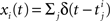denotes the ith unbinned, continuous-time spike train with spike event times (i = 1,…,N, j ∈ ℕ). The model we propose for z(t) is that of a CPP

where the event times t_j constitute a Poisson process, and the marks a_j are i.i.d. integer-valued random variables, drawn independently for all t_j (Figure 1 , left). The marks a_j determine the number of neurons that fire at time t_j, and will be referred to as the “amplitude” of the event at time t_j. The probability that an event has a specific amplitude is determined by the amplitude distribution f_A, i.e., f_A(ξ) = Pr{a_j = ξ} for all j ∈ ℕ (Figure 1 , top right). The Poisson process that generates the events t_j is called the “carrier process” of the model and its rate ν is the “carrier rate”. Processes of this type are also referred to as generalized, or marked, Poisson processes (see e.g., Snyder and Miller, 1991 for a general definition, and Ehm et al., 2007 for an alternative application to spike train analysis).

With the above model, the generation of a population of spike trains proceeds in two steps. First, realize a Poissonian carrier processes m(t) = Σ_jδ(t = t_j) and draw for each of its events t_j an i.i.d. amplitude a_j from the amplitude distribution f_A. In the second step, assign the spike at t_j to a_j individual processes, where the process IDs are determined from a separate “assignment distribution”. The simplest scenario assumes uniform assignment, where the a_j neuron IDs that receive the spike at t_j are drawn randomly from {1,…,N}, resulting in a homogeneous population. As CuBIC only aims for a lower bound on the order of correlation, irrespective of the neuron IDs that realize these correlations, we here ignore the assignment distribution, and focus on the amplitude distribution only. The following theorem clarifies the relationship between cumulant correlations and the amplitude distribution in the framework of the CPP (see Staude et al., 2009 for a proof).

Theorem 2 Let be a CPP with amplitude distribution f_A and carrier rate ν, and let X = (X₁,…,X_N) be the vector of counting variables obtained from the x_i(t) with bin width h. Then:

1. The components of X have correlations of order m (in the sense of Definition 1) if and only if f_A assigns non-zero probabilities to amplitudes ≥m.

2. With 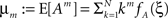, the cumulants of Z are given as

Note that correlations in the above theorem are measured strictly on the basis of the discretized counting variables X_i. As a consequence, they do not resolve (and do not depend on) the perfect temporal precision of the coincident events in the CPP. That is, if the events of z(t) were assigned to the individual processes with a temporal jitter that is small with respect to the bin size h, the effect of the jitter on the correlations is negligible.

Now let ξ ≤ N be the maximal order of correlation in the model, i.e., f_A(k) = 0 for k > ξ, and denote by ν_k (k = 1,…ξ) the compound rates of events of amplitude k, i.e., ν_k = ν·f_A(k). Then Eq. 3 can be written as

where , , and 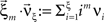is the vector dot product.

CuBIC

This section summarizes the stationary version of CuBIC to the extent that is needed to understand its adaptation to non-stationary populations (see Staude et al., 2009 for details). In brief, CuBIC quantifies the following thought experiment. Consider the situation of four simultaneously recorded neurons, where all neuron pairs have a correlation coefficient of c = 1. As c = 1 implies identity for all pairs of spike trains, all four spike trains must in fact be identical. In the framework of the CPP, this translates to the existence of events of amplitude a_j = 4, and hence correlation of order 4 (Theorem 1). This illustrates that it is possible, in principle, to infer the existence of fourth order correlations from estimated pairwise correlations. In Staude et al. (2009) , this inference was generalized by a hierarchy of statistical hypothesis tests , labeled by the order m of the correlation estimated from the population spike count, and the test parameter ξ, which indicates the maximal order of correlation allowed in the null hypothesis. For given m and ξ, the rejection of a hypothesis means that estimated correlations of order m in the data imply the presence of correlations of at least order ξ + 1. Combining tests for different values ξ then provides 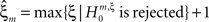as a lower bound on the order of correlation in the data. In the thought experiment above, we estimated pairwise correlation, hence m = 2, and rejected tests with ξ = 1,2,3, such that . In principle, the order of the estimated correlation m is a free parameter. However, as shown in Staude et al. (2009) , tests with m = 3 are already extremely sensitive, such that we will present both the stationary CuBIC and the non-stationary adaptation only for the case m = 3.

Assume one is given the first three cumulants of a population spike count variable Z′. Then, for a fixed value of the test parameter ξ, consider the following constrained maximization problem

subject to κ₂[Z′] = κ₂[Z]

κ₁[Z′] = κ₁[Z]

f_A(k) = 0 for k > ξ,

where Z is the population spike count of a model with parameters ν and f_A. The model that solves Eq. 5 has the maximal third cumulant, i.e., triplet correlations, among all models that do not have any correlations beyond order ξ, and have the same population-averaged first- and second-order properties, i.e., firing rates and pairwise correlations, as the given spike count variable Z′. As a consequence, implies that the third order correlations in Z′ cannot be realized with correlations of orders ≤ξ. Thus Z′ must have correlations of order ≥ξ + 1.

To solve Eq. 5, we use Eq. 4 and obtain the equivalent problem

In Eq. 6, the objective function and the constraints depend linearly on the model parameters . Problems of this type, so-called Linear Programming Problems, are uniquely solvable, e.g., by the Simplex Method or any of its variants (Press et al., 1992 , Chapter 10.8). The solution yields an upper bound for the third cumulant and the corresponding parameter vector . As it turns out, the only non-zero components of the solver are and , i.e., for all k ∉{1,ξ} (see The Solution of the Maximization in Appendix). The carrier rate and amplitude distribution of the CPP that maximizes Eq. 6 are then given by and .

With the solution of Eq. 5, the null hypothesis is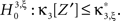

To test a sample against , we estimate its cumulants by the so-called k-statistics k_m (Stuart and Ord, 1987 ; the well-known sample mean and unbiased sample variance are the first two k-statistics). To derive the required distribution of the test statistic k₃ under , we assume that Z′ is the population spike count of the model with parameters and , i.e., the solution of Eq. 6 after the unknown cumulantsκ₁[Z′] andκ₂[Z′] have been replaced by their estimates k₁ and k₂. Thus, under the distribution of has expectation value , and its variance is given as (e.g., Stuart and Ord, 1987)

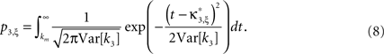
where κ_i[Z′] are the cumulants of Z′, obtained by inserting ν* and into Eq. 3. Finally, with sample sizes of L > 10000 (corresponding to a data set of 10 s duration, sampled with a bin width of h = 1 ms), the distribution of k₃ is well approximated by a normal distribution, such that the p-value of is given by

As mentioned above, the rejection of a specific hypothesis implies that the data have correlations beyond order ξ or, in other words, that ξ + 1 is a lower bound for the order of correlation. The final result of CuBIC is the maximum of these lower bounds

where α is a predefined test level (see Staude et al., 2009 for details).

The Non-Stationary Case

The Model

In the previous section, the CPP was presented as a model for populations with constant firing rates. However, (co-)variations in firing rate are a common feature of neuronal populations. To incorporate potential non-stationarities into the CPP, recall its central ingredients: the intensity of the population is described by the carrier rate ν, the population-averaged correlation structure is determined by the amplitude distribution f_A, and the precise composition of spikes and correlations within the population is determined by the assignment distribution. Given this parametrization, non-stationarities can in principle be included into the CPP by allowing a time-dependent carrier rate, amplitude distribution, assignment distribution, or combinations thereof.

Rather than presenting a general model for non-stationary populations, the focus of this study is to adapt the analysis technique CuBIC for potential variations in the firing rates. CuBIC, however, aims only at the population-average correlation structure f_A, and inference is based on the population spike count Z. Time dependencies in the assignment distribution only change the neuron IDs that realize correlations over time, but do no alter the order of correlations. As a consequence, the population spike count Z is not influenced by potential temporal variations of the assignment distribution (see Figure 2 A). Furthermore, CuBIC aims only at a lower bound for the maximal order of correlation, not on the precise values of correlations of different orders. As such, it aims for the largest entry with non-zero probability in the amplitude distribution, irrespective of whether this entry was present in the whole data stretch or if it occurred only within a short period. Taken together, CuBIC is blind for non-stationarities in the amplitude distribution and the assignment distribution. We therefore assume both these objects to be constant over time and consider only time-varying carrier rates ν(t) (see top panels in Figures 2 B,C).

FIGURE 2

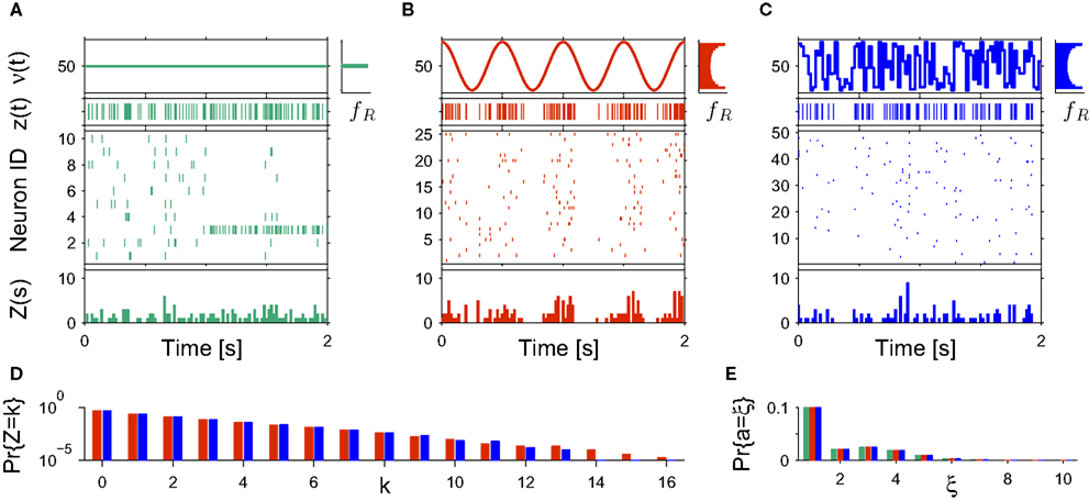
Figure 2. Non-stationarities in the CPP. Panels (A–C) show carrier rates ν(t) in Hz (top panels), the distributions of the bin-wise mean carrier rates (“carrier distributions” f_R, small panels on the right; bin size h = 20 ms), the event-times of the carrier process z(t) (second panels from top), raster plots (third panels from top) and population spike counts Z(s) (bottom panels) for three different data sets. (A) Time varying assignment distribution produces non-stationary single processes, although the carrier process z(t) is stationary (constant carrier rate ν(t) = 50 Hz; all carrier events with t_j < 1 s are assigned randomly, all carrier events with t_j ≥ 1 and amplitude a_j = 1 are assigned to neuron 3). (B) Cosine carrier rate results in non-stationary carrier process z(t), the subsequent uniform assignment to N = 25 neurons generates a homogeneous, non-stationary population. (C) The carrier rate is constant in bins of length h = 20 ms and subsequent values of ν(t) are i.i.d. realizations with the carrier distribution of the cosine carrier rate in (B). Carrier events in (C) are assigned uniformly to N = 50 neurons. As illustrated by the virtually identical population spike count distributions shown in (D) (estimated from 1000 s of artificial data, color code as in B,C; note logarithmic y-scale), the differences in both the carrier rate, in particular the temporal order of the bins, and the assignment, in particular the number of neurons of the generated population, do not influence the statistics of the population spike count Z. (E) Amplitude distributions of all three data sets are superpositions of a “background-peak” at ξ = 1 and a binomial distribution B(10,0.3) (color code as in A–C).

Cumulants of the Non-Stationary CPP

To relate the model parameters to the cumulants of Z for time varying ν(t), observe that the value of Z(s) in the window [sh,(s + 1)h) does not depend on the precise time course of the carrier rate ν(t) in this window, but only on the integral Substituting the carrier rate ν(t) with a piecewise constant function whose value in the interval [sh,(s + 1)h) is R_s thus results in an identical population spike count Z. Furthermore, CuBIC ignores the temporal order of Z(1),…,Z(L) and assumes subsequent values of Z to be i.i.d. variables. As a consequence, CuBIC is also blind for the temporal order of the rate values R_s, and we therefore assume them to be i.i.d. with a common “carrier distribution” f_R (compare panels B and C of Figure 2 ).

The above setting characterizes the population spike count Z as a parameter-dependent random variable, where the outcome of Z in the sth bin depends not only on the outcome of the CPP realization, but also on the (random) value of the rate variable R_s. For such “doubly stochastic” variables, the raw moments are given as

where the inner expectation is the expectation value of Z^m for a given value of the rate R, and the outer expectation is with respect to the distribution f_R. Now recall the definition of the moments as the coefficients of the Taylor series expansion of the characteristic function

such that the moments can be obtained from ɸ_Z via

Analogously, cumulants are the coefficients of the logarithm of the characteristic function

such that

A straightforward strategy to relate cumulants to moments is to insert Eq. 11 into the right hand side of Eq. 12, writing the logarithm as a power series, and collecting coefficients for identical powers of s. This procedure illustrates in particular that the mth cumulant is a function of the first m raw moments only, and, reversely, that the mth moment can be expressed as a function of the first m cumulants. We denote the maps relating cumulants to moments and moments to cumulants by F_m and G_m, respectively, such that

With these maps at hand, the mth cumulant of the non-stationary CPP can be computed by the following procedure.

1. For i = 1,…,m express the conditional moment μ_i[Z | R] in terms of the first i cumulants, i.e., write

μ_i[Z | R] = F_i(κ₁[Z | R],…,κ_i [Z | R]).

2. Apply Eq. 3 to the individual cumulants, such that μ_i[Z | R] = F_i(μ₁Rh,…,μ_iRh), where, as before, μ_i = μ_i[A] are the moments of the amplitude distribution f_A.

3. Compute the mth cumulant of Z by applying G_m

The results are summarized as the “law of total cumulance”. The first three orders read

A similar parameter transformation that leads from Eq. 3 to Eq. 4 simplifies Eqs. 18–20. In slight abuse of notation, we use the same symbol for the expected compound rates as for the constant compound rates of Eq. (4), i.e., write ν_k: = f_A(k)·κ₁[R]. Using the standardized cumulants of the rate variable and the vector notation and , Eqs. 18–20 can be written as

CuBIC for Non-Stationary Data

To adapt CuBIC to non-stationary populations, we need to formulate the general maximization problem (Eq. 5) for the case of time-dependent carrier rates. Using Eqs. 21–23 instead of Eq. 4, we obtain

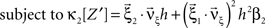
with , β₂ ∈ [0,∞) and β₃ ∈ (−∞,∞). After some algebra and substitution of the unknown cumulants κ_i[Z′] by their estimates k_i, we arrive at the equivalent problem

As opposed to the Linear Programming Problem of the stationary case (Eq. 6), the constraints in Eq. 25 do not apply to all free variables: the third standardized cumulant of the rate variable β₃ can, in principle, be arbitrarily large. As a consequence, also the objective function in Eq. 25 is unbounded. We therefore have to impose additional constraints on the carrier distribution f_R in order to ensure convergence of the maximization. The approach taken here is to prescribe a two-dimensional parametric family for the distribution of the rate variable, such that its third (standardized) cumulant can be expressed in terms of its first two cumulants. The choice for the family of carrier distributions determines the form of the objective function. Let us present two specific cases (see Section “Discussion” for more details on the role of this choice).

Symmetric carrier distributions

If the carrier distribution is symmetric about its mean, like e.g., the uniform distribution, we can exploit the fact that the third cumulant κ₃[R] of symmetric distributions vanishes ¹ . As a consequence, also β₃ = κ₃[R]/κ₁[R]³ = 0. The objective function of the maximization problem (Eq. 25) for symmetric carrier distributions thus becomes

This objective function is linear in the (expected) compound rates ν_k (k = 1,…,ξ) and quadratic in β₂. As the constraints are also linear, using Eq. 26 as the objective function in Eq. 25 yields a convex quadratic maximization problem. Problems of this type have a unique solution, and effective implementations of numerical solvers are available.

Gamma-distributed carrier rate

If the carrier variable R follows a Gamma-distribution, the third cumulant can be expressed in terms of the first two as . For the normalized third cumulant β₃ we thus have . The objective function then reads

As for symmetric carrier distributions, the objective function in Eq. 25 is linear in the expected component rates ν_k (k = 1,…,ξ) and quadratic in β₂. Thus, the resulting problem is also a convex quadratic programming problem and can be solved with the same solvers.

We wish to stress once again that the choice made here concerns only the family of the carrier distribution, not its particular shape. That is, if we chose e.g., a uniform distribution, we only determine that κ₃[R] = 0 but do not fix the support of the distribution. Finally, we note that the only non-zero components of the solution to the maximization problem are and , i.e., for all k ∉{1,ξ}, as in the stationary case (see The Solution of the Maximization in Appendix).

Variance of test statistic

As a final ingredient, CuBIC requires the variance of the test statistic k₃ in order to be able to compute the p-values. Assuming that the solution of Eq. 25 is available, we compute the second, fourth and sixth cumulant of the solution by inserting the solving and into the algorithm leading to Eq. 17. Plugging these cumulants into Eq. 7 yields Var[k₃], the variance of the test statistic k₃ under the non-stationary null-hypothesis. Insertion into Eq. 8 yields the corresponding p-value.

Case Studies

To illustrate the application of the adapted CuBIC, we consider here two typical experimental situations. In the first situation, data are recorded in early sensory systems, where characteristic firing rate profiles closely follow the stimulus. In such a scenario, information about the rate distribution can be obtained from the type of the stimulus. In the second situation, there is no direct relation between the experimental paradigm and non-stationarities in firing rates. In this case, ad hoc assumptions of the family of carrier rate are the only option. We illustrate both scenarios and the steps required when applying the non-stationary version of CuBIC by analyzing simulated spike trains.

Stimulus-Driven Non-Stationarity

Pure non-stationarity

Our first example mimics a recording in visual cortex with a oriented sinusoidal grating as stimulus. We model the population response in such an experiment by a CPP model with sinusoidal carrier rate ν(t), i.e.,

where B is the offset, C ≤ B is the amplitude of the modulation, ω is the temporal frequency of the stimulus and d is the phase, i.e., the sum of the stimulus phase and the delay it takes for the stimulus-driven activity to propagate to the recording electrodes (Figure 3 , top panels of left and right columns). The first data set of this example models the case of pure rate non-stationarity (Figure 3 , left column). The amplitude distribution is a delta-peak at ξ = 1, such that all events of the marked process z(t) have amplitude a_j = 1. As a consequence, z(t) is a simple Poisson process with rate ν(t). Setting B = C = 500 and ω = 500 ms, d = 0, and assigning the carrier spikes uniformly to a population of N = 50 spike trains, we obtain a homogeneous population where each neuron oscillates with a temporal frequency of 2 Hz, assuming firing rates between 0 and 20 Hz (second panel from top of Figure 3 , left). Note that assigning the events of z(t) to individual spike trains was done only for illustrative purposes, as it does not influence the results of CuBIC.

FIGURE 3

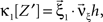
Figure 3. Population statistics and CuBIC results for cosine-like non-stationarity for three data sets. Shown are the carrier rate ν(t) (top panels), raster plots of N = 50 spike trains (second panels from top) and population spike counts Z(s) obtained with a bin width of length h = 5 ms (third panels from top) for the first 2 s of a data stretch of length T = 100 s. Below are the empirical distributions f_Z(k) = Pr{Z = k} estimated from the entire data set (second panel from bottom; blue bars: linear y-scale with axes on the left, green solid line: logarithmic y-scale with axes on the right). Bottom panels show p-values of the stationary CuBIC (green), the adapted CuBIC with cosine-like rate variations (red) and with bimodal rate variations (blue), where rejected null-hypotheses, i.e., p-values below a significance level of α = 0.05, are marked by arrowheads. Outlined bars and arrowheads in bottom panel show results of data where interspike intervals below 2 ms were removed before the analysis. Data with pure rate non-stationarity (left column) have a sinusoidal carrier rate ν(t) (top panel) and an amplitude distribution with mass concentrated at ξ = 1 (f_A(k) = 0 for k > 1; see text for details). Pure correlation (middle column) is modeled with a stationary carrier rate and correlation up to order 7 (ν(t) = const., f_A(k) = 0 for k∉{1,7}). The probability for the high-amplitude events results in a pairwise correlation coefficient of c = 0.01 if the events of the carrier process are distributed uniformly among the processes N = 50. The combined data set with non-stationarity and correlation (right column) has the same correlation structure as the data in the middle column, and the same carrier rate as in the first column.

To analyze the data, we chose a bin size of h = 5 ms, computed the population spike count Z(s), and estimated its distribution f_Z(k) = Pr{Z = k} from a total simulation time of T = 100 s (Figure 3 , third and fourth panels from top, respectively). Note that the population spike count Z does not provide unambiguous information about the carrier rate. Next, we applied the stationary version of CuBIC with m = 3. That is, we ignored the apparent non-stationarities that are present in the data and computed p-values p_3,ξ for ξ = 1,…,7 as described in Section “CuBIC” (Figure 3 , green bars in bottom panel). We found that only the p-value with ξ = 1 fell below the chosen significance level of α = 0.05 (Figure 3 , green arrowhead in bottom left panel). Hence, was rejected while all hypotheses with ξ > 1 were retained. As a consequence, the stationary CuBIC yields (Eq. 9) as a lower bound for the maximal order of correlation. As the data do not contain correlations beyond those induced by the population-wide non-stationarity, the stationary CuBIC thus leads to false positive inference.

Application of the adapted CuBIC requires the specification of a parametric family of carrier distributions f_R (“carrier family”). We put ourselves in the position of an experimenter, to whom the carrier rate is unknown and cannot be estimated directly; the only observable quantity is the population activity, which is a combination of the carrier rate and potential events of high amplitude. However, as the stimulus was a cosine, we assume also the carrier rate to be a cosine as in Eq. 28, only that the parameters B, C and d are unknown (ω can be estimated from the stimulus frequency). Now recall that the adaptation of CuBIC does not require knowledge of the exact time-course of the carrier rate: what matters is a model for the distribution of the average rate values in the bins Given h << 1/ω, we can assume that the sequence of rate values R_s samples the cosine faithfully, such that both the phase offset d and the oscillation frequency ω do not influence f_R. In this case, the moments (and cumulants) of all orders can be computed from the parameters B and C in a straightforward manner (see Cumulants of Carrier Distributions in Appendix). In our example, f_R is symmetric, which implies β₃ = 0 (see Symmetric Carrier Distributions). Furthermore, as the carrier rate ν(t) has to be non-negative, the model parameters must satisfy B ≥ C, which implies β₂ ≤ 1/2. The red bars of the lower left panel in Figure 3 show the p-values computed from Eq. 8, after (a) the solution of stationary problem, , has been substituted with the solution of Eq. 25 with objective function Eq. 26 and additional constraint β₂ ≤ 1/2, and (b) Var[k₃] was computed with the algorithm explained in Section “Variance of Test Statistic” with the cumulants of the rate variable R given in Section “Cumulants of Carrier Distributions ” in Appendix. We find that p_3,ξ > 0.05 for all ξ = 1,…,7, hence no hypothesis is rejected and the lower bound is . Thus, the adapted CuBIC does not infer correlation in this data set, and the adaptation successfully corrects for the faulty inference of correlation of the stationary version.

Reduced sensitivity in stationary data?

In the first data set, the stationary CuBIC assigned the rate-generated correlation among the counting variables X_i to events of amplitude ≥2. Allowing for potential (co-)variations of firing rates in the adapted CuBIC corrected for this faulty inference of correlations. Mathematically, allowing for rate (co-)variations allows non-zero values of the parameter β₂ in the maximization of the third cumulant (Eq. 25). Maximizing over a larger parameter space may then increase as compared to the stationary maximum . Thus, hypotheses that are rejected by the stationary CuBIC may be retained by the adapted version, as the latter can produce larger maximal third cumulants for a given value of ξ. Consequently, we expected the adapted version to be generally less sensitive for existing events of high amplitude. To investigate this issue, we generated a data set of pure correlation by choosing a constant carrier rate, but allowing for events of amplitude ξ_syn = 7 on top of the “background spikes” with ξ = 1 (Figure 3 , middle column). The probability of these events was set to f_A(7) = 0.0125, which resulted in a average pairwise correlation coefficient of c = 0.01 if the events of z(t) were assigned homogeneously to a population of N = 50 spike trains. The value for ν = 500 Hz was chosen to match the average carrier rate of the first example. Note that the additional events of amplitude ξ = 7 resulted in a slight increase of the population spike count from κ₁[Z] = κ₁[R]hμ₁ = 500·0.005·1 = 2.5 in the first example to κ₁[Z] ≈ 500·0.005·1.0753 ≈ 2.7 in this example, and thereby also increased the firing rates of the N = 50 spike trains. The remaining parameters in this and all following examples were: bin width h = 5 ms, simulation time T = 100 s.

Compared to the size of the population (N = 50), the rate of the high-amplitude events (ν₇ = κ₁[I]·f_A(7) ≈ 6 Hz) is relatively small. As a consequence, these are hardly visible in the raster displays and population spike counts (Figure 3 , second and third panels from top in the middle column). In the distributions of the population spike count, they lead to a slight increase for the frequency of patterns of size k ≈ 10, visible only on a logarithmic scale (Figure 3 , middle column, green solid line in fourth panel from top).

In this data set, the stationary CuBIC rejects all hypotheses up to a value of ξ = 6. Hence, CuBIC performs optimally in this data set, as the resulting lower bound corresponds to the maximal order of correlation ξ_syn = 7 in this data set.

To our big surprise and satisfaction, p-values for the adapted version of CuBIC were very similar to those of the stationary CuBIC (Figure 3 , bottom panel in middle column, red and green bars respectively). In particular, the adapted CuBIC rejected the same hypotheses, and, as a consequence, also yielded the same lower bound Contrary to our assumption, the proposed adaptation thus did not compromise CuBIC’s sensitivity in this stationary data set.

Combined effects

Finally, we generated a third data set that combined the properties of the first two examples (Figure 3 , right column). The amplitude distribution was the same as in the example of pure correlation, i.e., with an additional entry at ξ_syn = 7, while the carrier rate was the same cosine as in the data with pure non-stationarity (Figure 3 , top panels of right and left columns, respectively).

For this data set, we expected the stationary CuBIC to overestimate the order of correlation, i.e., to yield , as the considerable rate co-variation produces correlation among the X_i in addition to the events of high amplitude (Staude et al., 2008 ). To the contrary, however, p-values for the stationary CuBIC fell below the significance level only up to ξ = 4 (Figure 3 , green arrowheads in the bottom panel of the left column), yielding . Allowing for cosine-like non-stationarities in the null-hypotheses reduces the lower bound to (Figure 3 , red arrowheads in the bottom panel of the left column). Thus, rather than a false positive inference of correlation, the additional non-stationarity resulted in a reduction of the inferred order of correlation as compared to the stationary scenario.

Different carrier family

To investigate the robustness of the proposed adaptation with respect to faulty choices for the carrier family, we also analyzed the data under the assumption that the carrier rate switches between a state of low rate, ν_min, and of high rate, ν_max. This can be described by a bimodal carrier distribution

f_R(ν;ν_min,ν_max,η) = (1 − η)δ(ν − ν_min) + ηδ(ν − ν_max),

where δ(ν) is the Dirac-delta function and η∈[0,1] parametrizes the relative proportion of bins where ν(t) is in the low (high) rate state. Inspecting the time course of Z(s), we chose the mass of the two peaks identical (η = 0.5), which leaves a two-parameter family for f_R (its cumulants are derived in Section “Cumulants of Carrier Distributions” in Appendix). For the data shown in Figure 3 , allowing for such drastic rate dynamics hardly changed p-values as compared to the cosine carrier rate (compare red with blue bars in bottom panel of Figure 3 ). Most importantly, the bimodal adaptation resulted in the same lower bounds as the cosine adaptation.

Internally Generated Non-Stationarities

Gamma-distributed carrier rate

In the examples of the previous section, we inferred the type of non-stationarity from the experimental paradigm, i.e., from the properties of the stimulus. In many experimental situations, such a priori assumptions on the rate variable cannot be justified, and changes in firing rates can have diverse statistical properties. General excitability of the tissue can change firing rates either in the form of slow drifts or abrupt transitions between so called up- and down-states. Furthermore, both local computations and additional cortical or sub-cortical inputs may change firing rates of the recorded population.

A further feature of the previous examples was that the carrier rate ν(t) changed rather slowly. As mentioned above, however, the temporal dynamics of the carrier rate does not influence the statistics required for CuBIC, i.e., the population spike count Z, as long as the distribution of the rate values per bin, f_R, is not altered. The carrier rate ν(t) of the second class of examples is a piecewise constant function that changes its value in subsequent bins, i.e.,

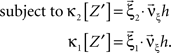
where L = T/h is the sample size (number of bins) Π_s(t) = 1 for t∈[sh,(s + 1)h) and Π_s(t) = 0 otherwise, and the R_s are the rate values drawn i.i.d. from the carrier distribution f_R (compare the model of rate-covariations in Staude et al., 2008 and the carrier rate in Figure 2 C). Here, f_R is a gamma distribution, i.e., where Γ(k) is the gamma function. As in the previous section, the parameters of the carrier rate (k and θ) are such that distributing the events of the carrier process z(t) uniformly among N = 50 spike trains leads to time varying firing rates λ(t) with mean value 10 Hz, and we set its variance to 40 Hz². The maximal value of λ(t) in the entire simulation was ≈79 Hz. The remaining parameters in the three examples shown in Figure 4 are as in those of Figure 3 . In data with pure rate non-stationarity (Figure 4 , left column) the amplitude distribution has an isolated peak at ξ = 1. For pure correlation (Figure 4 , middle column), the carrier rate is constant [ν(t) = 500 Hz] and the amplitude distribution has an additional peak at ξ_syn = 7 that resulted in a pairwise correlation coefficient of c = 0.01 among the N = 50 spike trains. Finally, the combined data set has the same time-varying carrier rate as the purely non-stationary data, and the same amplitude distribution as the data with pure correlation (Figure 4 , right column).

FIGURE 4

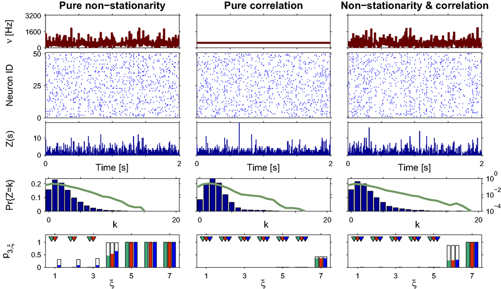
Figure 4. Population statistics and CuBIC results for non-stationarities with gamma-distributed carrier rate. The figure has the same setup as Figure 3 , only that the bottom panels show results for stationary CuBIC (green bars and arrowheads), allowed uniform carrier distribution (red bars and arrowheads) and gamma-distributed carrier rate (blue bars and arrowheads).

The gamma-distributed rate variable generates strongly fluctuating rate profiles, with peak values of the carrier rate above 3000 Hz. This leads to strong fluctuations in the population spike count even in the case of pure rate non-stationarity (Figure 4 , third panel from top in left column), such that its distribution has a fairly elongated tail (Figure 4 , fourth panel from top in left column).

Results of the stationary CuBIC

Despite quantitative differences, stationary CuBIC performs qualitatively similarly for gamma- and cosine-like carrier rate. For pure rate non-stationarity, it wrongly interprets the rate-induced correlations among the X_i as events of high amplitudes. The null-hypotheses are rejected up to ξ = 3, yielding a lower bound of (Figure 4 , green arrowheads in the bottom panel of the left column). Similarly, adding gamma-like non-stationarities to a data set with correlation decreases the inferred lower bound, here from in the stationary data (Figure 4 , green arrowheads in the bottom panel of the middle column) to in the non-stationary data (Figure 4 , green arrowheads in the bottom panel of the right column).

The adapted CuBIC

As opposed to Section “Stimulus-driven Non-stationarity” where properties of the carrier rate could be inferred from the stimulus, we here cannot make qualitative guesses about the type of non-stationarity. The fact that firing rates fluctuate on a bin-to-bin basis makes it very difficult to infer the type of non-stationarity from the raster plots, the population spike counts Z or its distribution f_Z. As a consequence, we can only make ad hoc assumptions on f_R. We consider two cases. First, we allow f_R to be a uniform distribution (Figure 4 , red bars and arrowheads in bottom panels). As the uniform distribution is symmetric, we use Eq. 26 as the objective function with the additional constraint β₂ ≤ 1/3 imposed by the non-negativity of the carrier rate. The cumulants of the uniform distribution (see Cumulants of carrier distributions in Appendix) are then used for the computation of Var[k₃]. Second, we allow for gamma-distributed non-stationarities, where we use Eq. 27 as the objective function and the cumulants of the gamma-distribution for the computation of Var[k₃] (Figure 4 , blue bars and arrowheads in bottom panels).

For the data with pure rate non-stationarity (Figure 4 , left column), allowing a uniform rate variable rejects hypotheses up to ξ = 3 and thus yields a lower bound of . Allowing f_R to be gamma-distributed, on the other hand, produces p-values above 0.05 for all ξ = 1,…,7, thereby retaining all hypotheses. Thus, while the uniform null-hypotheses fail to reduce the lower bound as compared to the stationary version, allowing for the true, gamma-distributed non-stationarities corrects for false positive inference of correlation.

For data with correlation, the choice of the carrier distribution has only little influence on the resulting p-values (Figure 4 , bottom panels in middle and left column). For pure correlation, the lower bounds are identical for all three rate models (). In the combined data set (Figure 4 , right column), the additional non-stationarity reduces the lower bound as compared to the stationary data with correlation to , irrespective of the non-stationarity allowed in the null-hypotheses.

Refractory Periods

Besides the stationarity, CuBIC’s second central assumption is that spike trains of single neurons can be described as Poisson processes, i.e., have exponential interspike interval (ISI) distributions. While tails of ISI distributions can often be relatively well described by exponentials, the high probability for short intervals of the Poisson process contradicts the absolute refractory period of a few milliseconds found in most nerve cells. We investigated the extent to which refractoriness influences test results of CuBIC by re-analyzing the data of the previous sections after short ISIs were removed. Specifically, for each data set we assigned the events of the carrier process randomly to the N = 50 spike trains, removed spikes of all spike trains that occurred with a temporal difference of τ ≤ 2 ms, and constructed the population spike counts of these thinned spike trains. The analysis of the refractory data showed that introducing refractoriness has a very limited effect on test results (outlined bars and arrowheads in lower panels of Figures 3 and 4 ). If p-values changed, they increased, which makes CuBIC more conservative but does not generate false positives. From all simulation, the increased p-value reduced the lower bound only in a single instance (cosine rate modulation with correlation, analyzed with stationary CuBIC at ξ = 4; green arrowhead in bottom right panel of Figure 3 ); in all remaining cases the refractory period changed p-values where they were above the significance level of α = 0.05. We thus conclude that CuBIC is reasonably robust if spike deviate from Poisson processes in terms of short refractory periods (here 2 ms).

Discussion

The analysis of massively parallel spike trains for higher-order correlations is a prerequisite for understanding the mechanisms of cooperative neuronal computation in the brain. However, analysis techniques to estimate higher-order correlations typically require enormous sample sizes, rendering the analysis of large (N > 10) populations for higher-order effects extremely difficult. In Staude et al. (2009) , we have presented a novel method (CuBIC) that avoids the need for extensive sample sizes. Numerical simulations illustrated that CuBIC reliably infers correlations of very high order (>10) from recordings of large (N ∼ 100), even weakly correlated neuronal populations (average pairwise correlation coefficient c < 0.01) with sample sizes corresponding to 10–100 s recording time.

As a statistical model, CuBIC assumes the CPP, where correlation among the spike trains is modeled by the insertion of additional coincident events (Ehm et al., 2007 ; Johnson and Goodman, 2007 ; Brette, 2009 ; Staude et al., 2010 ). The linear relation between the model parameters, i.e., the orders of correlation present in the data, and the cumulants κ_m[Z] of the population spike count Z allows the computation of the maximal value of κ_m[Z] under the assumption that the orders of correlation in the data do not exceed a predefined value ξ. Comparing the estimated cumulants to these upper bounds then yields a collection of statistical hypothesis tests , labeled by m, the order of the estimated cumulant, and ξ, the maximal order of correlation allowed in the null-hypothesis. In this paper, we chose a fixed value of m = 3, and for given ξ, the rejection of implies that the data must have correlations of order at least ξ + 1 (for a discussion on the choice of m see below). A combination of tests with different values for ξ finally yields a lower bound for the maximal order of correlation, denoted by . For a discussion of the properties and limitations of the CPP (e.g., positivity of correlations), general issues concerning CuBIC, and the relationship between cumulant-correlations and the higher-order parameters of the log-linear model used by, e.g., Martignon et al. (1995) , Schneidman et al. (2006) , Shlens et al. (2006) , we refer to the extensive discussion of Staude et al. (2009) . The latter point is discussed in more detail also in Staude et al. (2010 ). In this section, we focus on issues that relate directly to the novelties of the present study.

Before going into detail, we need to make a general remark. CuBIC is a parametric procedure, and assumes that the data, i.e., the population spike count, can be described sufficiently well by a discretized, potentially non-stationary CPP. If this model does not fit, results of CuBIC may be unreliable. The extent to which results are reliable then depends on the mismatch between the CPP and the data. In practice, where single spike trains deviate from Poisson processes, for example due to refractory properties, this mismatch may be evaluated by analyzing surrogate data (e.g., Grün, 2009 ). If, for instance, CuBIC returns in a data set of non-Poissonian spike trains, and the analysis of surrogate data with the same single process properties but without correlation yields , we can conclude that the value of is really due to existing correlations. This kind of analysis, however, has to be performed specifically for a given data set. As a first step, we have here investigated the effect of a spike train’s most obvious deviation from the Poisson process: absolute refractory periods (here 2 ms, Figures 3 and 4 ). Its relatively small effect on p-values makes us confident that CuBIC is a promising analysis method even if single spike trains deviate from the Poisson assumption. The detailed analysis of CuBIC’s robustness with respect to these violation is a central aspect of our current research (e.g., Staude et al., 2007 ; Reimer et al., 2009 ). We wish to stress that in the case of small bin sizes and hard refractory periods, assuming single processes to have Poisson statistics is essentially identical to the popular assumption of independence of subsequent bins in Bernoulli models (as in e.g., Martignon et al., 1995 ; Shlens et al., 2006 ). A more detailed discussion of this issue, together with an analysis of the parameter dependence of CuBIC can be found in Staude et al. (2009 ).

A central assumption in the original presentation of CuBIC (Staude et al., 2009 ) is that the statistics of the population does not change over time (stationarity). In the present study, we have adapted CuBIC to be able to analyze also non-stationary data. The basis of this adaptation is a non-stationary version of the CPP, where the intensity of the population, parametrized by the ν, is decoupled from the correlation structure, parametrized by the amplitude distribution f_A. Describing the population spike count as a doubly stochastic CPP, potential non-stationarities in the data can by integrated into the quantification of the null-hypotheses of CuBIC. We wish to stress once again, however, that non-stationarities in single neurons do not necessarily imply time varying carrier rates (see, e.g., Figure 2 A), such that not every non-stationary data set requires the application of the adapted CuBIC.

In this study, we presented the adaptation only for the third cumulant, i.e., m = 3. Although the derivation of the mathematical equations is straightforward also for higher values of m, the resulting expressions become increasingly complicated. This may result in particular in strong non-linearities in the maximization problem, such that additional care is necessary to ensure convergence of numerical solvers at the global maximum. Furthermore, the estimation of cumulants of order >3 becomes unreliable and their estimators have large variance, which may compromise test power. As CuBIC proved to be very sensitive even for m = 3 (Staude et al., 2009 ), we currently have not developed the theory for higher m. Nevertheless, this might be a fruitful direction of future research.

The main difference between the stationary CuBIC and its non-stationary adaptation lies in the maximization of the third cumulant of Z. Here, the adapted version requires that the third standardized cumulant β₃ = κ₃[R]/κ₁[R]³ of the binned carrier rate R does not assume arbitrary large values. In this study, this is achieved by prescribing a two-parameter family for the carrier distribution f_R (the “carrier family”). The remainder of this section is therefore primarily concerned with elucidating the role of this particular choice.

Correcting for Rate Effects

Classically, correlations are measured on a small time scale, and subsequently corrected for effects from the firing rates. The estimation of the firing rate, in turn, proceeds along one of the following two lines. Either, rate variations are identified with artifacts that are locked to the stimulus or some other external cue. Then, firing rates are estimated by averaging over repeated presentation of the stimulus, or trials (e.g., Perkel et al., 1967a ,b ; Aertsen et al., 1989 ). Alternatively, changes in firing rates are assumed to fluctuate only on slow time scales; they are then estimated by averaging over time. Although combinations, refinements and optimizations of both strategies have been developed (e.g., Grün et al., 2002b ; Ventura et al., 2005 ; Shimazaki et al., 2009 ), we wish to stress that all such corrections make strong a priori assumptions on the differences between “genuine” correlations and “artifacts” induced by non-stationary firing rates (see also Staude et al., 2008 ).

The correction of CuBIC, i.e. the choice of a carrier family, follows a fundamentally different strategy. Rather than assuming that firing rate profiles are identical over trials (first strategy) or that rate-fluctuations are band-limited (second strategy), the carrier family limits the extent to which correlations among the counting variables X_i are assigned to rate-variations. As discussed above, this choice ensures boundedness of the third standardized cumulant β₃ = κ₃[R]/κ₁[R]³ of the rate variable R. As κ₃[R] measures the skewness of the carrier distribution, large values of β₃ imply a long right tail. As a consequence, a population with large β₃ has bins with very large values of the carrier rate R. If binned firing rates can assume arbitrary high values, however, the difference between global rate variations and precise spike coordination vanishes. Thus, the choice of the carrier family determines the extent to which one assigns patterns with high spike counts to (co-)variations of firing rates. In other words: the carrier family sets CuBICs demarcation line between rate co-variation and genuine correlation.

In Section “Case Studies”, we illustrated how CuBIC operates in two alternative scenarios. In Section “Stimulus-driven Non-stationarity”, we assumed that properties of the firing rates can be inferred from the stimulus. Here, the stimulus was a cosine, but the reasoning there can be generalized to a broad class of stimuli. The effect of oriented bars, for instance, might be modeled by a bimodal carrier distribution as in Section “Different Carrier Family”,

where the mixing parameter η determines the relative duration of the respective stimulus phases (light/dark). The carrier family of Eq. 29 also describes experiments with a well-defined stimulus onset, as e.g., odor presentation or whisker stimulation. In such a scenario, η has to be chosen as the relative duration of the stimulus-off/stimulus-on epoch. Furthermore, properties of the carrier family in “free viewing” conditions might be estimated from the statistical properties of the visual scene.

In the second scenario (see Internally Generated Non-stationarities), the experimental paradigm did not provide information about the carrier family. Here, we argued that ad hoc assumptions are the only option. However, if the activity of individual neurons is available, their statistics can provide additional information that can be exploited. If, for instance, individual spike trains do not show evidence of time varying firing rates, or provide upper bounds for the cumulants of their firing rates, this information may be extrapolated to the level of the carrier rate. Together with general moment inequalities (e.g., Kumar, 2002 ), such information may help to dispose of the explicit choice of the carrier family by providing an explicit upper bound for β₃. Although the absence of a precise parametric model for the carrier distribution impedes the faithful computation of Var[k₃] under , the close similarity of the error-bars in Figure 5 A for the different methods makes us confident that Var[k₃] can be reasonably approximated by any carrier distribution as long as the upper bound is faithful (see also Section ‘What is the “true” Carrier Family?’ for conceptual issues concerning the choice for f_R).

FIGURE 5

Figure 5. Results of the maximization (Eq. 25 with appropriate objective functions) for data with pure correlation (see legend of Figure 3 for parameters). (A) Normalized variance of the rate variable that solves Eq. 25 for ξ = 1,…,7 for different types of allowed non-stationarities (green: stationary CuBIC; red: non-stationary CuBIC allowing uniform carrier distribution; blue: non-stationary CuBIC allowing gamma carrier distribution). (B) The maximal third cumulant as a function of the test parameter ξ for different types of allowed non-stationarities (same color code as in A). Error bars denote , corresponding to a significance level of α ≈ 0.05, the dashed line is the value of the test statistic k₃ and arrowheads denote rejected null-hypothesis where 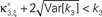(compare bottom panel of middle column in Figure 4 ).

Discussion of Case Studies

The analysis of artificial data (Figures 3 and 4 ) can be summarized by four major points:

1. For data with pure firing rate non-stationarity but no higher-order correlations, the stationary CuBIC misinterprets the common rate variations as events of amplitude ≥2, i.e., as correlations. The order of the inferred correlation depends on the kind of non-stationarity in the data ( for cosine carrier rate, for gamma-distributed rate variable).

2. Allowing for potential non-stationarities in the null-hypotheses can reduce this lower bound. Using the correct family for the carrier distribution, i.e., a cosine-like model for the data in Figure 3 and a gamma-distribution for the data in Figure 4 , corrects entirely for the false positive inference of the stationary CuBIC, such that the lower bound becomes . Choosing the wrong family, however, may not account properly for rate variations, especially if the family assigns smaller values of β₃ (e.g., allowing a uniform carrier distribution if the data had a gamma-distributed carrier rate as in Figure 4 ).

3. For stationary data with correlation, allowing for non-stationarities in the null-hypotheses has no effect on the inferred lower bound. This result holds irrespective of the type of non-stationarity allowed in the null-hypotheses.

4. Non-stationarities in data with correlation reduce the inferred lower bound as compared to data with the same correlation structure but constant firing rates. The degree of reduction depends mostly on the kind of non-stationarity in the data. The family allowed for the carrier distribution did not affect the lower bound.

It is well-known that co-variations in firing rates induce correlations between spike counts. Thus, it comes as no surprise that analyzing non-stationary data with the stationary CuBIC generates false positives (point 1). In the adaptation, parts of the correlation can be assigned to (co)-variations in firing rates. Allowing for non-stationarities therefore corrects for this faulty inference (point 2).

To understand why the adaptation did not generally reduce the lower bound (point 3), we investigated the interplay between the constraints and the objective function in the maximization of the third cumulant in further detail. Due to the increased number of degrees of freedom, our intuition was that allowing for non-stationarities additional to the correlations of order ξ would simply increase the maximal value of the third cumulant as compared to the stationary version. This, however, seems not to be the case. In the data sets with pure correlation (Figures 3 and 4 , middle panels), for example, the values of and are identical for ξ ≥ 4 (Figure 5 B shows results for stationary, uniform and gamma-distributed rate variables, results of combined data sets are very similar, data not shown). The reason is that for a given value of the first estimated cumulant k₁, the constraint penalizes stronger non-stationarity, i.e., larger values of the standardized variance β₂, with a reduction of the (expected) component rates ν₁,…,ν_ξ, and vice versa. In the objective function (Eq. 25)

the component rates enter via , while the β₂-dependence is a parabola with negative curvature. As

especially for large values of ξ, the objective function profits more from high component rates than the constraint penalizes these. As a consequence, the maximization favors high component rates over strong rate fluctuations, especially for large ξ. The results of the maximization procedure for the data with pure correlation supports this interpretation, as the standardized variance of the model that maximizes κ₃[Z], , decreases with ξ (Figure 5 A). For ξ ≥ 4, we have , and, as a consequence, the maximizing model of the adapted maximization problem is the same as that of the stationary maximization. Consequently, also the solutions and the p-values are identical. Contrary to our initial intuition, the maximization thus does not generally favor strong rate variations. Evidently, however, the extent to which the inclusion of non-stationarities in the null-hypothesis alter test results depends crucially on the parameters of the data.

Parameter-Dependence of Test Results

The results of the case studies summarized above suggest that including potential non-stationarities in the null-hypothesis is always a safe bet: it corrects for false positive inference if correlation originates from rate effects, but does not alter p-values if the stationary CuBIC did not overestimate the order of correlation. To sketch the parameter range where including non-stationarities reduces p-values only if necessary, recall that we have identified the reason for the unchanged maximal third cumulant in the interplay between the constraint and the objective function. Considering the general objective function (Eq. 25) however, we find that the influence of the non-stationarity (via β₂ and β₃) depends on the value of the first sample cumulant k₁. For k₁ < 1, non-stationarities (positive β₂ and β₃) hardly influence the objective function, hence the maximization can be assumed to favor high component rates over non-stationarities, yielding identical test results for the stationary and the adapted CuBIC. For k₁ >> 1 a small increase in β₃ has a strong effect on the objective function, which may in turn favor strong non-stationarities, thereby producing different test results for the stationary and the adapted method. Thus, a crucial parameter for the performance of the adaptation is the first sample cumulant k₁. Now k₁ is the estimator of where λ_i is the (average) firing rate of the ith neuron. Thus, given the summed firing rate of the recorded population, we may chose the bin size h in order to keep k₁ in a range where the adaptation can be expected to have reasonable test power. As all simulations of Section “Case Studies” had k₁ ∼ 2.5, achieving a value of k₁ < 1 is not always necessary.

What is the “True” Carrier Family?

In Section “Correcting for Rate Effects” we have presented a few guidelines for the choice of the family of carrier rate distributions. There are cases, however, where this choice is not easily justifiable by resorting to observable quantities. To discuss the status of this problem in more depth, we wish to stress that measures of correlation and their various corrections are purely statistical in nature. To be of scientific value, statistical results have to be put in context and must be interpreted, e.g., in terms of biophysical mechanisms. The “firing rate” of a neuron, for example, is not a biophysical entity as such. The term arises only if one describes the variable behavior of a neuron using point processes. As a consequence, whether or not the choice of a chosen carrier family f_R is “valid” depends entirely on the intended biological interpretation. If, for example, the choice of f_R is guided by the properties of the stimulus, the natural interpretation of rejected null-hypothesis is that the dynamic properties of the neuronal network under investigation generates correlations beyond direct stimulus effects. In an alternative situation, f_R may be chosen to reflect the slow ongoing dynamics observed in a simultaneously recorded mass signal (as e.g., described in Tsodyks et al., 1999 ). Significant higher-order correlations are then interpreted as coordinated activity that is not covered by such large-scale phenomena. In either case, the term “correlations beyond the rate” is biologically meaningful only after an explicit interpretation of the term “rate” by the experimenter. Finally, we stress that the different choices for the carrier family affected the test results only weakly, especially if the data had genuine spike correlations (Figures 3 and 4 , left and right columns). Thus, a perfect match between the carrier distribution underlying a Monte Carlo simulation and the family assigned in CuBIC does not seem to be of great importance for a reliable interpretation of test results.

Appendix

List of symbols

The Solution of the Maximization

This Appendix shows that the solution of the stationary (Eq. 6) and the non-stationary maximization problem (Eq. 25) fulfills for k = 2,…,ξ − 1.

The non-stationary problem (Eq. 25) has the objective function

with constraints

Simple computations starting from Eqs. 33 and 34 yield

which, after insertion into Eq. 32 yield

with

Now for k = 2,…,ξ − 1 we have

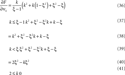
The gradient of the objective function therefore points to negative values of ν_k for k = 2,…,ξ − 1. Because ν_k ≥ 0, the maximum is achieved for ν_k = 0. In the stationary maximization problem, insertion of the constraints into the objective function yields the same F as Eq. 35, only with H = k₂(ξ + 1). Consequently, Eqs. 36–41 hold also in the stationary scenario.

Cumulants of Carrier Distributions

For the computation of Var[k₃] (Eq. 7) from the solutions of the maximization procedure, i.e., the parameters and , we require explicit expressions for the cumulants of the carrier distribution f_R up to order m = 6. Recall that we here considered only two-dimensional parametric families for f_R, which implies that these parameters can be computed from the known mean value and the normalized variance . In the following, we provide explicit expressions that relate the raw moments to these parameters. Expressions for the cumulants are then computed by applying the conversion map G constructed in Section “Cumulants of the Non-stationary CPP”.

Cosine carrier rates

For ν(t) = B + Ccos(2Π ω t + d), we derive the distribution of the rate values 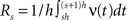under the assumption that subsequent values of R_s sample the cosine faithfully. In this case, we can express R as a function of the [0,1]-uniform variable T as R = g(T), with g(t) = B + Ccos(T). Denoting the uniform distribution by f_T, the distribution function of R is thus given by

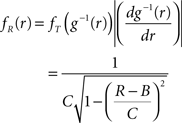
The first six moments can be computed by solving the integrals

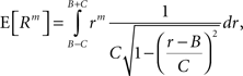
which yields

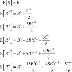
Bimodal carrier rates

Let f_R(ν;ν_min,ν_max,η) = (1 − η)δ(ν − ν_min) + ηδ(ν − ν_max) be a bimodal rate distribution, where η∈[0,1] and ν_min,ν_max ∈ [0,∞]. The raw moments of f_R are

Uniform carrier rates

If R is uniformly distributed between a and b, the raw moments of R are given as

Gamma carrier rates

The moments of the gamma distribution 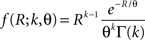with parameters k and θ are given as

where Γ denotes the gamma-function.

Conflict of Interest Statement

The authors declare that the research was conducted in the absence of any commercial or financial relationships that could be construed as a potential conflict of interest.

Acknowledgments

We are grateful to Stuart Baker for a fruitful discussion, Leona Schild for help in the initial phase of this project, and Imke Reimer for comments on an earlier version of the manuscript. Supported by the German Federal Ministry of Education and Research (BMBF grants 01GQ0420 and 01GQ01413 to the BCCN Freiburg and Berlin), the Helmholz Alliance on Systems Biology (Germany), and SFB 780.

Footnote

1. ^ Generally, κ3[R] is a measure for the skewness of fR, such that κ3[R] < 0 for left- skewed, κ3[R] = 0 for symmetric, and κ3[R] > 0 for right-skewed distributions.

References

Abbott, L. F., and Dayan, P. (1999). The effect of correlated variability on the accuracy of a population code. Neural Comput. 11, 91–101.

Pubmed Abstract | Pubmed Full Text | CrossRef Full Text

Abeles, M. (1991). Corticonics: Neural Circuits of the Cerebral Cortex, 1st Edn. Cambridge: Cambridge University Press.

Aertsen, A., Gerstein, G., Habib, M., and Palm, G. (1989). Dynamics of neuronal firing correlation: modulation of “effective connectivity”. J. Neurophysiol. 61, 900–917.

Pubmed Abstract | Pubmed Full Text

Averbeck, B. B., Latham, P. E., and Pouget, A. (2006). Neural correlations, population coding and computation. Nat. Rev. Neurosci. 7, 358–366.

Pubmed Abstract | Pubmed Full Text | CrossRef Full Text

Averbeck, B. B., and Lee, D. (2006). Effects of noise correlations on information encoding and decoding. J. Neurophysiol. 95, 3633–3644.

Pubmed Abstract | Pubmed Full Text | CrossRef Full Text

Bair, W., Zohary, E., and Newsome, W. (2001). Correlated firing in macaque visual area MT: time scales and relationship to behavior. J. Neurosci. 21, 1676–1697.

Pubmed Abstract | Pubmed Full Text

Bohte, S. M., Spekreijse, H., and Roelfsema, P. R. (2000). The effects of pair-wise and higher-order correlations on the firing rate of a postsynaptic neuron. Neural Comput. 12, 153–179.

Pubmed Abstract | Pubmed Full Text | CrossRef Full Text

Brette, R. (2009). Generation of correlated spike trains. Neural Comput. 21, 188–215.

Pubmed Abstract | Pubmed Full Text | CrossRef Full Text

Brown, E. N., Kaas, R. E., and Mitra, P. P. (2004). Multiple neural spike train data analysis: state-of-the-art and future challenges. Nat. Neurosci. 7, 456–461.

Pubmed Abstract | Pubmed Full Text | CrossRef Full Text

Darroch, J., and Speed, T. (1983). Additive and multiplicative models and interactions. Ann. Stat. 11, 724–738.

CrossRef Full Text

Del Prete, V., Martignon, L., and Villa, A. E. P. (2004). Detection of syntonies between multiple spike trains using a coarse-grain binarization of spike count distributions. Network 15, 13–28.

Pubmed Abstract | Pubmed Full Text | CrossRef Full Text

Diesmann, M., Gewaltig, M.-O., and Aertsen, A. (1999). Stable propagation of synchronous spiking in cortical neural networks. Nature 402, 529–533.

Pubmed Abstract | Pubmed Full Text | CrossRef Full Text

Di Nardo, E., Guarino, G., and Senato, D. (2008). A unifying framework for k-statistics, polykays and their multivariate generalizations. Bernoulli 14, 440–468.

CrossRef Full Text

Ecker, A. S., Berens, P., Keliris, G. A., Bethge, M., Logothetis, N. K., and Tolias, A. S. (2010). Decorrelated neuronal firing in cortical microcircuits. Science 327, 584–587.

Pubmed Abstract | Pubmed Full Text | CrossRef Full Text

Eggermont, J. J. (1990). The Correlative Brain, Vol. 16, Studies of Brain Function. Berlin: Springer-Verlag.

Ehm, W., Staude, B., and Rotter, S. (2007). Decomposition of neuronal assembly activity via empirical de-poissonization. Electron. J. Stat. 1, 473–495.

CrossRef Full Text

Fujisawa, S., Amarasingham, A., Harrison, M., and Buzsaki, G. (2008). Behavior-dependent short-term assembly dynamics in the medial prefrontal cortex. Nat. Neurosci. 11, 823–833.

Pubmed Abstract | Pubmed Full Text | CrossRef Full Text

Gardiner, C. W. (2003). Handbook of Stochastic Methods for Physics, Chemistry and the Natural Sciences, 3 Edn. Springer Series in Synergetics, Vol. 13. Berlin: Springer.

Gerstein, G. L., Bedenbaugh, P., and Aertsen, A. (1989). Neuronal assemblies. IEEE Trans. Biomed. Eng. 36, 4–14.

Pubmed Abstract | Pubmed Full Text | CrossRef Full Text

Gray, C. M., and Singer, W. (1989). Stimulus-specific neuronal oscillations in orientation columns of cat visual cortex. Proc. Natl. Acad. Sci. U.S.A. 86, 1698–1702.

Pubmed Abstract | Pubmed Full Text | CrossRef Full Text

Grün, S. (2009). Data-driven significance estimation of precise spike correlation. J. Neurophysiol. 101, 1126–1140 (invited review).

Pubmed Abstract | Pubmed Full Text | CrossRef Full Text

Grün, S., Diesmann, M., and Aertsen, A. (2002a). ‘Unitary Events’ in multiple single-neuron spiking activity. I. Detection and significance. Neural Comput. 14, 43–80.

CrossRef Full Text

Grün, S., Diesmann, M., and Aertsen, A. (2002b). ‘Unitary Events’ in multiple single-neuron spiking activity. II. Non-Stationary data. Neural Comput. 14, 81–119.

CrossRef Full Text

Hebb, D. O. (1949). The organization of behavior: a neuropsychological theory. New York: John Wiley & Sons.

Johnson, D., and Goodman, I. (2007). Jointly Poisson processes. arXiv:0911.2524.

Josić, K., Shea-Brown, E., Doiron, B., and de la Rocha, J. (2009). Stimulus-dependent correlations and population codes. Neural Comput. 21, 2774–2804.

Pubmed Abstract | Pubmed Full Text | CrossRef Full Text

Kohn, A., and Smith, M. A. (2005). Stimulus dependence of neuronal correlations in primary visual cortex of the Macaque. J. Neurosci. 25, 3661–3673.

Pubmed Abstract | Pubmed Full Text | CrossRef Full Text

König, P., Engel, A. K., and Singer, W. (1996). Integrator or coincidence detector? The role of the cortical neuron revisited. Trends Neurosci. 19, 130–137.

Pubmed Abstract | Pubmed Full Text | CrossRef Full Text

Kreiter, A. K., and Singer, W. (1996). Stimulus-dependent synchronization of neuronal responses in the visual cortex of awake macaque monkey. J. Neurosci. 16, 2381–2396.

Pubmed Abstract | Pubmed Full Text

Kuhn, A., Aertsen, A., and Rotter, S. (2003). Higher-order statistics of input ensembles and the response of simple model neurons. Neural Comput. 1, 67–101.

CrossRef Full Text

Kumar, P. (2002). Moments inequalities of a random variable defined over a finite interval. J. Ineq. Pure Appl. Math. 3, 41.

Martignon, L., Deco, G., Laskey, K., Diamond, M., Freiwald, W., and Vaadia, E. (2000). Neural coding: higher-order temporal patterns in the neurostatistics of cell assemblies. Neural Comput. 12, 2621–2653.

Pubmed Abstract | Pubmed Full Text | CrossRef Full Text

Martignon, L., von Hasseln, H., Grün, S., Aertsen, A., and Palm, G. (1995). Detecting higher-order interactions among the spiking events in a group of neurons. Biol. Cybern. 73, 69–81.

Pubmed Abstract | Pubmed Full Text | CrossRef Full Text

Montani, F., Ince, R. A. A., Senatore, R., Arabzadeh, E., Diamond, M. E., and Panzeri, S. (2009). The impact of high-order interactions on the rate of synchronous discharge and information transmission in somatosensory cortex. Philos. Trans. R. Soc. Lond. A 367, 3297–3310.

CrossRef Full Text

Nakahara, H., and Amari, S. (2002). Information-geometric measure for neural spikes. Neural Comput. 14, 2269–2316.

Pubmed Abstract | Pubmed Full Text | CrossRef Full Text

Perkel, D. H., Gerstein, G. L., and Moore, G. P. (1967a). Neuronal spike trains and stochastic point processes. I. The single spike train. Biophys. J. 7, 391–418.

CrossRef Full Text

Perkel, D. H., Gerstein, G. L., and Moore, G. P. (1967b). Neuronal spike trains and stochastic point processes. II. Simultaneous spike trains. Biophys. J. 7, 419–440.

CrossRef Full Text

Pillow, J. W., Shlens, J., Paninski, L., Sher, A., Litke, A. M., Chichilnisky, E. J., and Simoncelli, E. P. (2008). Spatio-temporal correlations and visual signalling in a complete neuronal population. Nature 454, 995–999.

Pubmed Abstract | Pubmed Full Text | CrossRef Full Text

Press, W. H., Teukolsky, S. A., Vetterling, W. T., and Flannery, B. P. (1992). Numerical Recipes in C, 2 Edn. New York, NY: Cambridge University Press.

Reimer, I. C. G., Staude, B., and Rotter, S. (2009). “Detecting assembly activity in massively parallel spike trains,” in Proceedings of the 8th Meeting of the German Neuroscience Society/30th Göttingen Neurobiology Conference, Vol. 1, Neuroforum, Supplement, eds H. Bähr and I. Zerr. Heidelberg: Spektrum Akademischer Verlag.

Riehle, A., Grün, S., Diesmann, M., and Aertsen, A. (1997). Spike synchronization and rate modulation differentially involved in motor cortical function. Science 278, 1950–1953.

Pubmed Abstract | Pubmed Full Text | CrossRef Full Text

Roudi, Y., Nirenberg, S., and Latham, P. E. (2009). Pairwise maximum entropy models for studying large biological systems: when they can work and when they can’t. PLoS Comput. Biol. 5, e1000380. doi: 10.1371/journal.pcbi.1000380.

Pubmed Abstract | Pubmed Full Text | CrossRef Full Text

Sakurai, Y., and Takahashi, S. (2006). Dynamic synchrony of firing in the monkey prefrontal cortex during working-memory tasks. J. Neurosci. 6, 10141–10153.

CrossRef Full Text

Schneidman, E., Berry, M. J., Segev, R., and Bialek, W. (2006). Weak pairwise correlations imply strongly correlated network states in a neural population. Nature 440, 1007–1012.

Pubmed Abstract | Pubmed Full Text | CrossRef Full Text

Shadlen, M. N., and Newsome, W. T. (1998). The variable discharge of cortical neurons: implications for connectivity, computation, and information coding. J. Neurosci. 18, 3870–3896.

Pubmed Abstract | Pubmed Full Text

Shimazaki, H., Amari, S., Brown, E. N., and Grün, S. (2009). “State-space analysis on time-varying correlations in parallel spike sequences,” in Proceedings of the IEEE International Conference on Acoustics, Speech, and Signal Processing (ICASSP) (Washington, DC: IEEE Computer Society), 3501–3504.

Shlens, J., Field, G. D., Gauthier, J. L., Grivich, M. I., Petrusca, D., Sher, A., Litke, A. M., and Chichilnisky, E. J. (2006). The structure of multi-neuron firing patterns in primate retina. J. Neurosci. 26, 8254–8266.

Pubmed Abstract | Pubmed Full Text | CrossRef Full Text

Snyder, D. L., and Miller, M. I. (1991). Random Point Processes in Time and Space. New York: Springer.

Softky, W. R. (1995). Simple codes versus efficient codes. Curr. Opin. Neurobiol. 5, 239–247 (commentary).

Pubmed Abstract | Pubmed Full Text | CrossRef Full Text

Staude, B., Grün, S., and Rotter, S. (2010). “Higher order correlations and cumulants,” in Analysis of Parallel Spike Trains, eds S. Grün and S. Rotter. Springer Series in Computational Neuroscience. Berlin: Springer-Verlag.

Staude, B., Rotter, S., and Grün, S. (2007). “Detecting the existence of higher-order correlations in multiple single-unit spike trains,” in Abstract Viewer/Itinerary Planner, Vol. 103.9/AAA18 (Washington, DC: Society for Neuroscience).

Staude, B., Rotter, S., and Grün, S. (2008). Can spike coordination be differentiated from rate covariation? Neural Comput. 20, 1973–1999.

Pubmed Abstract | Pubmed Full Text | CrossRef Full Text

Staude, B., Rotter, S., and Grün, S. (2009). CuBIC: cumulant based inference of higher-order correlations. J. Comput. Neurosci. doi: 10.1007/s10827-009-0195-x.

Pubmed Abstract | Pubmed Full Text | CrossRef Full Text

Stratonovich, R. L. (1967). Topics in the Theory of Random Noise. New York, Gordon & Breach Science.

Streitberg, B. (1990). Lancaster interactions revisited. Ann. Stat. 18, 1878–1885.

CrossRef Full Text

Stuart, A., and Ord, J. K. (1987). Kendall’s Advanced Theory of Statistics, 5 Edn. London: Griffin and Co.

Tsodyks, M., Kenet, T., Grinvald, A., and Arieli, A. (1999). Linking spontaneous activity of single cortical neurons and the underlying functional architecture. Science 286, 1943–1946.

Pubmed Abstract | Pubmed Full Text | CrossRef Full Text

Vaadia, E., Aertsen, A., and Nelken, I. (1995). ‘Dynamics of neuronal interactions’ cannot be explained by ’neuronal transients’. Proc. Biol. Sci. 261, 407–410.

Pubmed Abstract | Pubmed Full Text | CrossRef Full Text

Vaadia, E., Haalman, I., Abeles, M., Bergman, H., Prut, Y., Slovin, H., and Aertsen, A. (1995). Dynamics of neuronal interactions in monkey cortex in relation to behavioural events. Nature 373, 515–518.

Pubmed Abstract | Pubmed Full Text | CrossRef Full Text

Ventura, V., Cai, C., and Kass, R. E. (2005). Trial-to-trial variability and its effect on time-varying dependency between two neurons. J. Neurophysiol. 94, 2928–2939.

Pubmed Abstract | Pubmed Full Text | CrossRef Full Text