Error-based analysis of optimal tuning functions explains phenomena observed in sensory neurons

Introduction

Behaving organisms often exhibit optimal, or nearly optimal performance (e.g., Jacobs, 1999; Ernst and Banks, 2002; Jacobs et al., 2009), despite physiological constraints and noise which is inherent to both the environment and the neural activity. Experimental work performed over the past few years has suggested that one means by which such effective behavior is achieved is through adaptation to the environment occurring across multiple time scales (e.g., milliseconds – Wang et al., 2005; seconds – Dean et al., 2008; minutes – Pettet and Gilbert, 1992). A major challenge pertaining to such results relates to the construction of a coherent theoretical framework within which the efficacy of such adaptation processes can be motivated and assessed. We believe that a carefully articulated reverse engineering perspective (see Marom et al., 2009), based on the utilization of well founded engineering principles, can yield significant insight about these phenomena. More specifically, such approaches can explain how the environmental state may be effectively estimated from the neural spike trains and from prior knowledge through a process of neural decoding. Within this context, many psychophysical and neurophysiological results can be explained by Bayesian models, suggesting that organisms may indeed be employing Bayesian calculations in their decision-making (Knill and Richards, 1996; Knill and Pouget, 2004; Rao, 2004; Ma et al., 2006). Optimal real-time decoding methods have been proposed over the past decade for static (Zemel et al., 1998; Deneve et al., 2001; Pouget et al., 2002, 2003; Averbeck et al., 2006; Ma et al., 2006; Beck et al., 2008) and dynamic (Twum-Danso and Brockett, 2001; Eden et al., 2004; Beck and Pouget, 2007; Huys et al., 2007; Pitkow et al., 2007; Deneve, 2008; Bobrowski et al., 2009) environments. While much of this work has been performed in the context of sensory systems, it has also been widely used in the context of higher brain regions (e.g., hippocampus – Barbieri et al., 2004; Eden et al., 2004), and may therefore be relevant across multiple physiological levels.

Given the well developed theory of Bayesian decoding, an intriguing follow-up question relates to the properties of optimal encoding methods, namely determining the properties of a neural population in the sensory layer that optimizes performance, subject to physiological constraints. Sensory neurons are often characterized by their tuning functions (sometimes referred to as “tuning curves” – e.g., Korte and Rauschecker, 1993; Anderson et al., 2000; Brenner et al., 2000; Dragoi et al., 2000; Harper and McAlpine, 2004), which quantify the relationship between an external stimulus and the evoked activities of each neuron, typically measured by the probability, or frequency, of emitting spikes. From an ecological point of view it is speculated that optimal tuning functions are not universal, but rather adapt themselves to the specific context and to the statistical nature of the environment. The neurophysiological literature offers much experimental evidence for neurons in many areas, which respond to changes in the statistical attributes of stimuli by modulating their response properties (e.g., Pettet and Gilbert, 1992; Brenner et al., 2000; Dragoi et al., 2000; Dean et al., 2005; Hosoya et al., 2005).

Theoretical studies of optimal tuning functions hinge on the notion of optimality, which requires the definition of an appropriate cost function. Arguably, a natural cost function is some measure of distance between the true and the estimated environmental state. In this context a reasonable choice is the mean squared error (MSE), or the average Euclidean distance between the two signals. While other distance measures can be envisaged, and should indeed be studied in appropriate contexts, there are many advantages to using this specific measure, not least of which is its relative analytic tractability. The optimality criterion then becomes minimal MSE (MMSE), where it is assumed that the spike trains generated by the sensory cells are later processed by an optimal decoder. Unfortunately, even in this relatively simple setting, analytical examination of the dependence of the MMSE on the tuning functions is infeasible in the general case, and many researchers draw conclusions about optimality of tuning functions from lower bounds on the MSE, especially those which make use of Fisher information (Seung and Sompolinsky, 1993; Pouget et al., 1999; Zhang and Sejnowski, 1999; Eurich et al., 2000; Harper and McAlpine, 2004; Johnson and Ray, 2004; Seriès et al., 2004; Lánskỳ and Greenwood, 2005; Brown and Bäcker, 2006; Toyoizumi et al., 2006). Unfortunately, in many cases reaching conclusions based on, often loose, bounds can lead to very misleading results, which stand in distinct opposition to predictions arising from analyzing the MMSE itself (see Discussion). Along different lines, other researchers consider information theoretic quantities (Brunel and Nadal, 1998; Panzeri et al., 1999; McDonnell and Stocks, 2008; Geisler et al., 2009; Nikitin et al., 2009), attempting to determine conditions under which the maximal amount of information is conveyed, subject to various constraints. However, a direct relation (as opposed to bounds) between such quantities and the MSE has only been established in very specific situations (Duncan, 1970; Guo et al., 2005) and does not hold in general. As far as we aware, Brunel and Nadal (1998) were the first to obtain an optimal width in the MMSE sense, for triangular tuning functions in a special case where the entire population emits a single spike. Interestingly, they showed that the error based result differs from the one based on mutual information, although a qualitative similarity was noted. Other notable exceptions are the work of Bethge et al. (2002, 2003), who employed Monte Carlo simulations in order to assess the MMSE directly in specific scenarios, and the work of Bobrowski et al. (2009), who computed the MMSE analytically to find optimal tuning functions in a concrete setting. We note that in the context of two-dimensional rate-based coding, MMSE-optimal receptive fields were investigated by Liu et al. (2009), who focused on the relationship between ganglion cell mosaics and receptive field shapes irregularities.

In this paper we directly address the issue of MMSE-optimal tuning functions, using well-justified approximations which lead to explicit analytic results. We examine various scenarios, including some that were not previously treated, and make novel predictions that can be tested experimentally. We begin in Section “Fisher-Optimal Width” by analyzing optimality in terms of Fisher information and demonstrate why drawing qualitative and quantitative conclusions based on bounds can be misleading. In fact, bound-based predictions can sometimes be diametrically opposed to the predictions based on the true error. This notion is of great importance due to the very prevalent use of approximations and bounds on the true error. We then move in Section “MMSE-Based Optimal Width” to discuss the implications of directly minimizing the MMSE, focusing on the effects of noise and multimodality. The advantages of dynamic real-time modification of tuning function properties are analyzed in Section “Dynamic Optimal Width”, and concrete experimental predictions are made. In fact, some of these predictions have already been observed in existing experimental data. Specifically, we predict that neuronal tuning functions possess an optimal width, which increases with prior uncertainty and environmental noise, and decreases with the decoding time window. The results of the paper are summarized and discussed in Section “Discussion”, and the mathematical details appear in Section “Materials and Methods”.

Materials and Methods

We investigate the problem of neural encoding and decoding in a static environment. More formally, consider an environment described by a random variable X, taking values in some space χ, and characterized by a probability density function p(·) (in order to simplify notation, we refrain from indexing probability distributions with the corresponding random variable, e.g., p_X(·), as the random variable will be clear from the context). In general, X may represent a stochastic dynamic process (e.g., Bobrowski et al., 2009) but we limit ourselves in this study to the static case. In typical cases X may be a random vector, e.g., the spatial location of an object, the frequency and intensity of a sound and so on. More generally, in the case of neurons in associative cortical regions, X can represent more abstract quantities. Suppose that X is sensed by a population of M sensory neurons which emit spike trains corresponding to the counting processes where represents the number of spikes emitted by cell m up to time t. Denote by λ_m(·) the tuning function of the m-th sensory cell. We further assume that, given the input, these spike trains are conditionally independent Poisson processes, namely

implying that (in a more general case of dynamic tuning functions {λ_m(t, ·)}, with which we deal later, the parameter of the Poisson distribution is – see Bobrowski et al., 2009). Following this encoding process, the goal of an optimal decoder is to find the best reconstruction of the input X, based on observations of the M spike trains N_t. In this paper we focus on the converse problem, namely the selection of tuning functions for encoding, that facilitate optimal decoding of X.

We formulate our results within a Bayesian setting, where it is assumed that the input signal X is drawn from some prior probability density function (pdf) p(·), and the task is to estimate the true state X, based on the prior distribution and the spike trains N_t observed up to time t. For any estimator we consider the mean squared error where the expectation is taken over both the observations N_t and the state X. It is well known that the estimator minimizing the MSE, is given by the conditional mean 𝔼[X | N_t] (e.g., Van Trees, 1968), which depends on the parameters defining the tuning functions {λ_m(x)}.

As a specific example, assuming that the tuning functions are Gaussians with centers c₁, …, c_M and widths α₁, …, α_M, the estimator and the corresponding MMSE, depend on θ = (c₁, …, c_M, α₁, …, α_M). The optimal values of the parameters are then given by a further minimization process,

In other words, u^opt represents the tuning function parameters which lead to minimal reconstruction error. In this paper we focus on fixed centers of the tuning functions, and study the optimal widths of the sensory tuning functions that minimize MMSE(u).

Optimal Decoding of Neural Spike Trains

As stated before, the optimal estimator minimizing the MSE is given by . This estimator can be directly computed using the posterior distribution, obtained from Bayes’ theorem

where K is a normalization constant. We comment that here, and in the sequel, we use the symbol K to denote a generic normalization constant. Since such constants will play no role in the analysis, we do not bother to distinguish between them. For analytical tractability we restrict ourselves to the family of Gaussian prior distributions and consider Gaussian tuning functions

which in many cases set a fair approximation to biological tuning functions (e.g., Anderson et al., 2000; Pouget et al., 2000). From Eq. 1 we have

In the multi-dimensional case X ∼ 𝒩(m_x, Σ_x) and the Gaussian tuning functions are of the form

Bayesian Cramér–Rao Bound

Since the MMSE is often difficult to compute, an alternative approach which has been widely used in the neural computation literature is based on minimizing a more tractable lower bound on the MSE, related to Fisher information of the population of sensory neurons. The Fisher information is defined by

If X is deterministic, as in the classic (non-Bayesian) case, and is the estimation bias, then the error variance of any non-Bayesian estimator is lower bounded by which is the Cramér–Rao bound (Van Trees, 1968). The extension to the Bayesian setting, where X is a random variable with probability density function p(·), often referred to as the Bayesian Cramér–Rao bound (BCRB), states that

where and the bounded quantity is the MSE of any estimator (section 1.1.2 in Van Trees and Bell, 2007). Note that the expectation in Eq. 6 is taken with respect to both the observations N_t and the state X, in contrast to the non-Bayesian case where the unknown state X is deterministic. Note that in the asymptotic limit, t → ∞, the prior term, ℐ(p(x)), can be neglected with respect to the expected Fisher information, so that the asymptotic BCRB is 1/𝔼[𝒥(X)].

The second term in the denominator of Eq. 6 is independent of the tuning functions, and in the case of a univariate Gaussian prior is given by

In our setting, the expected value of the population’s Fisher information is given by

(see Section “Expectation of Population Fisher Information” in Appendix).

In the multi-dimensional case the right hand side of Eq. 6 is replaced by the inverse of the matrix J = 𝔼[𝒥(X)] + ℐ(p(x)), where

and the left hand side is replaced by the error correlation matrix The interpretation of the resulting inequality is twofold. First, the matrix R − J⁻¹ is non-negative definite and second,

where d is the dimension of X (Van Trees, 1968).

It is straightforward to show that in this case

The expression for 𝔼[𝒥(X)] is similar to Eq. 7 and is derived in Section “Expectation of Population Fisher Information” in Appendix, yielding

where ξ_m = (c_m − m_x)^T (A_m + Σ_x)⁻¹(c_m − m_x).

Analytical Derivation of the MMSE

We now proceed to establish closed form expressions for the MMSE. In order to maintain analytical tractability we analyze the simple case of equally spaced tuning functions (c_m+1 − c_M ≡ Δc) with uniform width (α_m ≡ α). When the width is of the order of Δc or higher, and M is large enough with respect to σ_x, the mean firing rate of the entire population is practically uniform for any “reasonable” X. As shown in Section “Uniform Mean Firing Rate of Population” in Appendix, the sum Σ_m λ_m(x) is well approximated in this case by Under these conditions the posterior (Eq. 3) takes the form

implying that [X | N_t] ∼ where

Recalling that the spike trains are independent Poisson processes, namely and in light of the above approximation, is independent of X and Y ∼ Pois(αt_eff), where Since the MMSE is given by

and thus we get an explicit expression for the normalized MMSE,

In the multivariate case we assume that the centers of the tuning functions form a dense multi-dimensional lattice with equal spacing Δc along all axes, and Eq. 10 becomes

namely [X | N_t] ∼ 𝒩 where

In this case (see Section “Uniform Mean Firing Rate of Population” in Appendix), and

Incorporation of Noise

Suppose that due to environmental noise the value of X is not directly available to the sensory system, which must respond to a noisy version of the environmental state – For simplicity we assume additive Gaussian noise: For a dense layer of sensory neurons the joint posterior distribution of the environmental state and noise is

which is Gaussian with respect to W, where Integration over w gives the marginal distribution

which is Gaussian with variance

where as before. The MMSE is computed directly from the posterior variance:

Note that when σ_w → ∞ the sensory information becomes irrelevant for estimating X, and indeed in such case

Multisensory Integration

Consider the case where the environmental state is estimated based on observations from two different sensory modalities (e.g., visual and auditory). The spike trains in each channel are generated in a similar manner to the unimodal case, but are then integrated to yield enhanced neural decoding. All quantities that are related to the first and second modalities will be indexed by v and a, respectively, although these modalities are not necessarily the visual and the auditory.

Each sensory modality detects a different noisy version of the environmental state: in the “visual” pathway and in the “auditory” pathway. The noise variables are Gaussian with zero-mean and variances and , respectively, and independent of each other as they emerge from different physical processes. The noisy versions of the environmental state are encoded by M_v + M_a sensory neurons with conditional Poisson statistics:

where the tuning functions in each modality are Gaussian with uniform width,

We assume that the tuning functions are dense enough, namely the widths are not significantly smaller than the spacing between the centers, and equally spaced

The full expression for the MMSE in this case is

where and (the derivation appears in Section “MMSE for Multisensory Integration” in Appendix).

Results

As argued in Section “Materials and Methods”, obtaining optimal tuning function parameters (or simply optimal width, in the simplified scenario presented in Section “Analytical Derivation of the MMSE”) requires computation of the MMSE for every given set of parameters, which is often not even numerically feasible. In the context of classical estimation, in order to maintain analytical tractability, the Cramér–Rao bound has been traditionally analyzed in place of the MMSE. In this text we employ a theoretical framework of optimal Bayesian estimation, in an attempt to find the optimal tuning functions that facilitate optimal estimation of X from the observations (the neural spike trains). We start by analyzing optimal width as predicted from the BCRB and proceed to scrutinize the properties of optimal width derived directly from the MMSE.

Fisher-Optimal Width

In a Bayesian context, it is well known (Van Trees, 1968) that for any estimator the MSE is lower bounded by the Bayesian Cramér–Rao lower bound (BCRB) given in Eq. 6. An interesting question is the following: considering that the MSE of any estimator (and thus the MMSE itself) is lower bounded by the BCRB, do the optimal widths also minimize the BCRB? In other words, can the BCRB be used as a proxy to the MMSE in selecting optimal widths? If this were the case, we could analyze MMSE-optimality by searching for widths that maximize the expected value of the Fisher information defined in Eq. 5. This alternative analysis would be favorable, because in most cases analytical computation of 𝔼[𝒥(X)] is much simpler than that of the MMSE, especially when the conditional likelihood is separable, in which case the population’s log likelihood reduces to a sum of individual log likelihood functions. Moreover, it remains analytically tractable under much broader conditions. Unfortunately, as we show below, the answer to the above question is negative. Despite the fact that for any encoding ensemble the BCRB bounds the MMSE from below, and may even approximate it in the asymptotic limit (if, for example, 𝒥(X) is independent of X), the behavior of the two (as a function of tuning function widths) is very different, as we demonstrate below.

In terms of the BCRB the existence of an optimal set of widths critically depends on the dimensionality of the environmental state. We consider first the univariate case, and then discuss the extension to multiple dimensions.

The univariate case

In the scalar case, using the tuning functions in Eq. 2, it follows from Eq. 7 that it is best to employ infinitesimally narrow tuning functions, since 𝔼[𝒥(X)] → ∞ most rapidly when α_m → 0 for all m, although Fisher information is undefined when one of the width parameters is exactly 0. A similar result was suggested previously for non-Bayesian estimation schemes (Seung and Sompolinsky, 1993; Zhang and Sejnowski, 1999; Brown and Bäcker, 2006), but within the framework that was employed there the result was not valid, as we elucidate in Section “Discussion”. Why does Fisher information predict that “narrower is better”? As a tuning function narrows, the probability that the stimulus will appear within its effective receptive field and evoke any activity decreases, but more and more information could be extracted about the stimulus if the cell did emit a spike. Evidently, in the limit α_m → 0 the gain in information dominates the low probability and BCRB → 0; however, this is precisely the regime where the bound vanishes and is therefore trivial. This result is in complete contrast with the MSE, which is minimal for non-zero values of α as we show below. More disturbingly, as argued in Section “The Univariate Case”, the performance is in fact the worst possible when α → 0.

We note that Bethge et al. (2002) were the first to address the shortcomings of lower bounds on the MSE in a Bayesian setting. These authors stressed the fact that performance bounds are usually tight only in the limit of infinitely long time windows, and cannot be expected to reflect the behavior of the bounded quantities for finite decoding times. They observed that, for any X, the minimal conditional MSE asymptotically equals 1/𝒥(X), and by taking expectations on both sides they obtained 𝔼[1/𝒥(X)] as the asymptotic value of the MMSE, which they assessed using Monte Carlo simulations.

The multivariate case

In this case, using the d-dimensional Gaussian tuning functions (Eq. 4) characterized by the matrices (A_m), the problem becomes more complex as is clear from Eq. 9, because the tuning functions may have different widths along different axes or even non-diagonal matrices. For simplicity we focus on the case where the matrices A_m are diagonal. By definition, the MSE of any estimator is the trace of its error correlation matrix, and in accordance with Eq. 8, Fisher-optimal tuning functions minimize the trace of J⁻¹, which equals the sum of its eigenvalues. If the widths in all dimensions are vanishingly small (A_m ≡ εI where ε ≪ 1), A_m becomes negligible with respect to Σ_x and In 3D and in higher dimensions the matrix is close to the zero matrix, and consequently the eigenvalues of 𝔼[𝒥(X)] are vanishingly small. If all widths are large (A_m ≡ (1/ε) I where ε ≪ 1), A_m dominates Σ_x and (c_m − m_x)^T], namely the eigenvalues of 𝔼[𝒥(X)] are still vanishingly small. This means that when the widths are too small or too large, the BCRB dictates poor estimation performance in high dimensional settings (specifically, the information gain no longer dominates the low probability in the limit of vanishing widths). Therefore, there exists an optimal set of finite positive widths that minimize the BCRB. As an exception, in 2D the eigenvalues of are finite when the widths approach 0, and 𝔼[𝒥(X)] cannot be said to have infinitesimally small eigenvalues. In fact, numerical calculations for radial prior distribution reveal that in 2D “narrower is still better”, as in the univariate case.

An interesting observation concerning the BCRB based optimal widths is that they cannot depend on the available decoding time t, since 𝔼[𝒥(X)] is simply proportional to t. As we will show, an important consequence of the present work is to show that the optimal tuning function widths, based on minimizing the MMSE, depend explicitly on time. In this sense, choosing optimal tuning functions based on the BCRB leads to a qualitatively incorrect prediction. We return to this issue in Section “Discussion”, where further difficulties arising from the utilization of lower bounds are presented.

MMSE-Based Optimal Width

Having discussed predictions about optimal widths based on BCRB minimization, we wish to test their reliability by finding optimal widths through direct MMSE minimization. As explained in Section “Materials and Methods”, in order to facilitate an analytic derivation of the MMSE, we examine here the case of dense equally spaced tuning functions with uniform widths. We consider first the univariate case and then proceed to the multivariate setting. As far as we are aware, Bethge et al. (2002) were the first to observe, using Monte Carlo simulations, that the MSE-optimal width of tuning functions may depend on decoding time.

The univariate case

Based on Eq. 11, we plot the normalized MMSE as a function of the width (Figure 1A) for different combinations of effective decoding time and prior standard deviation. The effective time, t_eff, defined in Section “Analytical Derivation of the MMSE”, is proportional to the time over which spikes accumulate. The existence of an optimal width, which is not only positive but also varies with σ_x and t_eff , is clearly exhibited. A similar result was first demonstrated by Bobrowski et al. (2009), but the dependence of optimal width on the two other parameters was not examined. Note that the derivation in Eq. 11 is not reliable in the vicinity of the y-axis, because the approximation of uniform population firing rate (see Analytical Derivation of the MMSE) is not valid when α → 0. Nevertheless, it can be proved that when α → 0, P(N_t = 0) → 1 and as a consequence and indeed

FIGURE 1

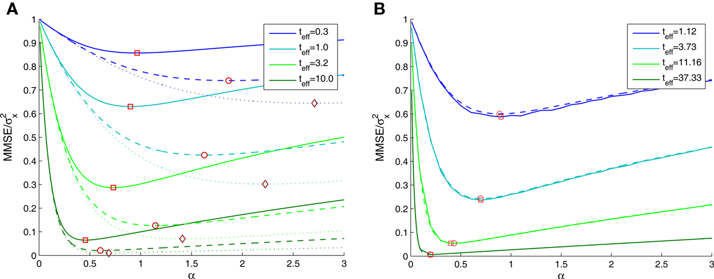
Figure 1. (A) The normalized MMSE of a dense population of Gaussian tuning functions against tuning function width, for different values of effective decoding time (shortest – uppermost triplet, longest – lowermost triplet). In each triplet three values of prior standard deviation were examined – σ_x = 1 (solid), σ_x = 2 (dashed), and σ_x = 3 (dotted), where the optimal width is indicated by squares, circles and diamonds, respectively. (B) The normalized MMSE for different values of effective decoding time (σ_x = 1), obtained theoretically (dashed lines, optimal width indicated by circles) and in simulation (solid lines, optimal width indicated by squares). Simulation parameters: N = 251, X ∈ [−4,4], M = 250, Δc = 0.034, λ_max = 50.

The existence of an optimal width is very intuitive, considering the tradeoff between multiplicity of spikes and informativeness of observations. When tuning functions are too wide, multiple spikes will be generated that loosely depend on the stimulus, and thus the observations carry little information. When tuning functions are too narrow, an observed spike will be informative about the stimulus but the generation of a spike is very unlikely. Thus, an intermediate optimal width emerges. To verify that the results were not affected by the approximation in Eq. 10, we compare in Figure 1B the theoretical MMSE with the MMSE obtained in simulations, which make no assumptions about uniform population firing rate. As can be seen in the figure, the two functions coincide, and in particular, the optimal widths are nearly identical. Recall that at each moment it is assumed that α is not significantly smaller than Δc (this is required for the uniform population firing rate approximation). For the values obtained in Figure 1A this implies Δc smaller than about 0.5. Obviously, the validity of Eq. 10 would break down for sufficiently long decoding time windows. For instance, when (i.e., when α^opt < 0.583Δc) the relative ripple of the population firing rate rises above 0.5% (see Section “Uniform Mean Firing Rate of Population” in Appendix). Nevertheless, as can be observed in Figure 1B, the theoretical approximation for the MMSE in Eq. 11 holds even for vanishing width, despite the non-uniformity in population firing rate (this appears more clearly in Figure 8).

We now turn to analyze the effect of the two parameters, σ_x and t_eff, in Eq. 11. The effective time is a measure for the number of spikes generated by the neural population, since it is proportional to λ_maxt (where λ_max is the maximal mean firing rate of a single neuron) and also to 1/Δc (which is proportional to the population size when the population is required to “cover” a certain fraction of the stimulus space). Longer effective times increase the likelihood of spikes under all circumstances, and therefore the drawback of narrow tuning functions is somewhat mitigated, leading to a reduction in optimal width (as illustrated in Figure 2A).

FIGURE 2

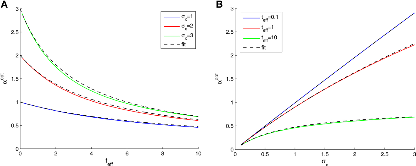
Figure 2. Optimal tuning functions width as a function of (A) effective decoding time, and (B) prior standard deviation. All curves are well-fitted by the same function:

The prior standard deviation reflects the initial uncertainty in the environment: the larger it is – the less is known a priori about the identity of the stimulus. Confidence about stimulus identity (associated with small MMSE) may stem from either a deterministic environment or from numerous observations for which the likelihood is very sharp. When the environment is less certain, many more observations are needed in order to obtain a narrow posterior distribution leading to smaller MMSE, and thus the optimal width increases (as illustrated in Figure 2B). Consider the condition discussed above for the uniform rate approximation to hold with high accuracy, namely Assuming, for example, that σ_x ≥ Δc, implies that t_eff ≤ 6/Δc suffices to guarantee the above condition. Under these conditions we obtain a simple empirical expression relating the optimal width to the effective time and prior uncertainty,

Figure 2 demonstrates the quality of this relation.

Finally, an interesting limit to consider is that of short decoding times. In this case the tuning functions are broad and the uniform sum rate approximation is expected to hold accurately. More precisely, when t → 0 the Poisson random variable converges in probability to a Bernoulli random variable with “success” probability αt_eff, in which case the expression for the normalized MMSE (Eq. 11) greatly simplifies,

Differentiating with respect to α and setting the result to 0 yields

Note that by taking the appropriate limit in the empirical formula (Eq. 18) we see that lim_t→0α^opt = σ_x, consistently with the above exact derivation.

Interestingly, when the width equals the prior standard deviation, the normalized MMSE can be calculated exactly for any effective time,

which for very short time windows converges to the optimal normalized MMSE.

The multi-dimensional case

We consider multivariate normal distributions for both the prior and the tuning functions. We start by considering a radial prior distribution and radial tuning functions, namely Gaussians with covariance matrices and A_m = α²I, respectively, where I is the d × d identity matrix. In this simple scenario the posterior covariance matrix in Eq. 13 becomes

where From Eq. 14 we see that

As long as the parameter of the Poisson random variable Y increases with the dimensionality d, in a manner that is equivalent to longer effective time (albeit width-dependent). Consequently, recalling (Eq. 18), the optimal width decreases with the dimensionality of the stimulus. Numerical calculations show that indeed this is the case in 2D and 3D for effective times which are not extremely long. This is in contrast with the predictions made by Zhang and Sejnowski (1999), where it was speculated that performance is indifferent to the width of the tuning functions in 2D, and improves with infinitely increasing width in higher dimensions.

When the prior covariance matrix and tuning functions shape matrix A are diagonal with, possibly different, elements and respectively, the MMSE is given by

where Since the random variable Y appears in every term in the sum, combined with different prior variances, the optimal width vector will adjust itself to the vector of prior variances, namely the optimal width will be largest (smallest) in the dimension where the prior variance is largest (smallest).

Biological implications

An important feature of the theoretical results is the ability to predict the qualitative behavior that biological tuning functions should adopt, if they are to perform optimally. From Eq. 18 we see that if the environmental uncertainty (expressed by σ_x) decreases, the tuning functions width is expected to reduce accordingly (this holds in 2D as well). This prediction provides a possible theoretical explanation for some results obtained in psychophysical experiments (Yeshurun and Carrasco, 1999). In these experiments human subjects were tested on spatial resolution tasks where targets appeared at random locations on a computer screen. In each trial the subjects were instructed to fixate on the screen center and the target was presented for a brief moment, with or without a preceding brief spatial cue marking the location of the target but being neutral with respect to the spatial resolution task. The authors found that the existence of the preceding cue improved both reaction times and success rates, concluding that spatial resolution was enhanced following the cue by reducing the size of neuronal receptive fields. Following their interpretation, we argue that the spatial cue reduces the uncertainty about the stimulus by bounding the region where the stimulus is likely to appear (i.e., σ_x is reduced). In light of our results, an optimal sensory system would then respond to the decrease in prior standard deviation by narrowing the tuning functions toward stimulus onset.

Our prediction may also relate to the neurophysiological experiments of Martinez-Trujillo and Treue (2004), who recorded the activity of direction-sensitive MT neurons in awake macaque monkeys in response to random dot patterns. These patterns appeared in two distinct regions of the visual field, one inside the neuron’s receptive field and another on the opposite hemifield, but both were governed by the same general movement direction. The direction-selective tuning function was measured when the animal’s attention was directed to a fixation point between these regions (“neutral”) and when its attention was directed to the other region with the same movement direction (“same”). In the “same” condition, neuronal response was enhanced near the tuning function center and suppressed away from the center with respect to the “neutral” condition, in a manner that is equivalent to a reduction in tuning function width (albeit followed by a modulation of maximal firing rate, which is fixed in our model). A possible interpretation is that attending the random dot pattern outside the receptive field and observing its movement direction strengthens the belief that the movement direction inside the receptive field is the same, thereby narrowing the prior distribution of directions and thus requiring narrow tuning functions.

The effect of environmental noise

In Figure 2B we saw that the optimal width increases with σ_x, the prior environmental uncertainty. Since external noise adds further uncertainty to the environment, we expect the optimal tuning functions to broaden with increasing noise levels, but the exact effect of noise is difficult to predict because even in the case of additive Gaussian noise with standard deviation σ_w the expression for the MMSE (Eq. 16) becomes slightly more complex. The optimal width in this case is plotted against effective time (Figure 3A) and against prior standard deviation (Figure 3B) for different values of noise levels. All curves are very well-fitted empirically by the function

where the average squared error of each fit is less than 1.3 × 10⁻³. This result implies that the effect of noise boils down to increasing the prior uncertainty. Since the noise is additive, and is independent of the stimulus, the term is precisely the standard deviation of the noisy stimulus meaning that the optimal width for estimating X is the same as for estimating This might not seem trivial by looking at Eq. 16, where the two standard deviations are not interchangeable, but is nonetheless very intuitive: seeing that all spikes depend only on it is the only quantity that can be estimated directly from the spike trains, whereas X is then estimated solely from the estimator of Therefore, optimal estimation of X necessitates first estimating optimally.

FIGURE 3

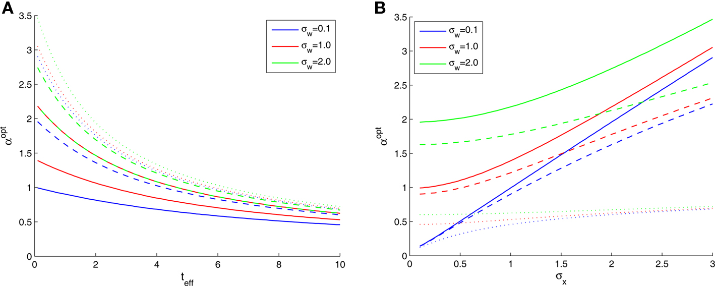
Figure 3. Optimal tuning functions width in the presence of noise, for different values of parameters: (A) σ_x = 1 (solid), σ_x = 2 (dashed), and σ_x = 3 (dotted); (B) t_eff = 0. 1 (solid), t_eff = 1 (dashed), and t_eff = 10 (dotted).

An indication for the symmetric role played by the prior and the noise, can be seen in Figure 3A, where the dashed red curve (σ_x = 2, σ_w = 1) merges with the solid green curve (σ_x = 1, σ_w = 2). Note also that the greatest effect of noise is observed when the prior standard deviation is small, whereas for large σ_x the relative contribution of noise becomes more and more negligible (Figure 3B).

The effect of multimodality

Integration of sensory information from different modalities (e.g., visual, auditory, somatosensory) has the advantage of increasing estimation reliability and accuracy since each channel provides an independent sampling of the environment (we focus here on the simple case where tuning functions are bell-shaped in all modalities). In the absence of noise, this improvement is merely reflected by an increased number of observations, but the main advantage manifests itself in the noisy case, where multimodal integration has the potential of noise reduction since the noise variables in the two modalities are independent. Considering two sensory modalities, denoted by v and a, and indexing the respective parameters of each modality by v and a, we provide a closed form expression for the MMSE in Eq. 17. When integrating the observations, the spike trains in each modality are weighted according to their reliability, reflected in the predictability of the stimulus based on the estimated input (related to σ_w,v, σ_w,a) and in the discriminability of the tuning functions (related to α_v, α_a). For instance, when “visual” noise has infinite variance or when “visual” tuning functions are flat, the spike trains in the “visual” pathway do not bear any information about the stimulus and are thus ignored by the optimal decoder. Indeed, when substituting σ_w,v = ∞ or α_v = ∞ in Eq. 17, it reduces to Eq. 16 with α_a, σ_w,a in place of α, σ_w. Note that in the absence of noise the MMSE reduces to which is identical to the unimodal expression for the MMSE with twice the expected number of observations (Y_v + Y_a ∼ Pois(α2t_eff)).

In a bimodal setting, the optimal width in each modality adapts itself to the standard deviation of the noise associated with that modality. To see that, we fix σ_w,v = 0.5, and plot the optimal widths against the ratio of noise standard deviations σ_w,a/σ_w,v (Figure 4A). When the “visual” channel is noisier (σ_w,a/σ_w,v < 1), the optimal “auditory” tuning functions are narrower than their counterparts, and when the “auditory” channel is noisier the situation is reversed. Interestingly, even when the “visual” noise variance is fixed, the optimal width in the “visual” modality is slightly affected by the “auditory” noise variance.

FIGURE 4

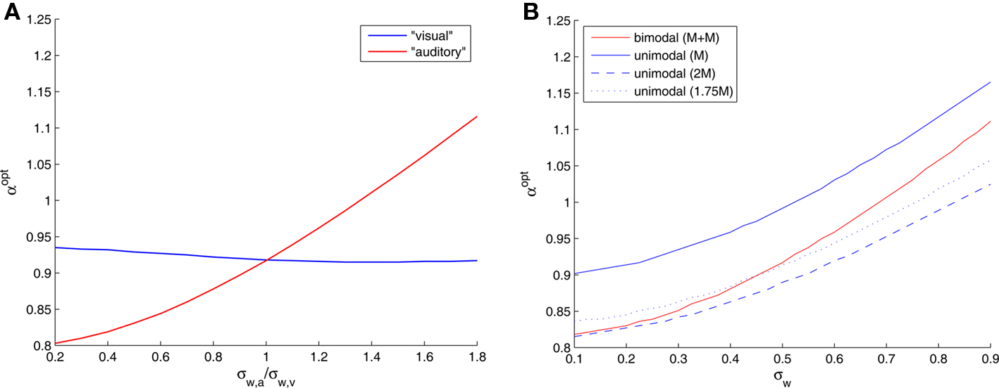
Figure 4. (A) Optimal tuning function widths in different sensory modalities as a function of the ratio between the noise standard deviations of the underlying physical phenomena (t_eff = 1, σ_x = 1, and σ_w,v = 0. 5). (B) Optimal tuning function widths in symmetrical bimodal and in unimodal settings (t_eff = 1 and σ_x = 1). The numbers in parentheses denote sizes of populations.

In the symmetric case we can easily compare the unimodal and bimodal settings. Assuming that the number of tuning functions in each modality is the same, integrating two modalities doubles the expected number of observations, naturally resulting in a smaller optimal width (Figure 4B). When the overall number of tuning functions is maintained constant, splitting them into two populations of equal size in each modality is preferred in terms of MMSE (results not shown), because the bimodal setting also has the advantage of partial noise-cancellation. But what can be said about the optimizing width in each setting? In Figure 4B we observe that 2M optimal tuning functions in a single modality are narrower than M + M optimal tuning functions for two different modalities. What is more intriguing is the fact that single-modality optimal tuning functions are still narrower than their double-modality counterparts even when they are outnumbered, as long as the noise standard deviation is sufficiently large.

Biological implications

The latter prediction may be related to experimental results dealing with multisensory compensation. Neuronal tuning functions are observed not only in the sensory areas but also in associative areas in the cortex, where cortical maps are adaptable and not strictly defined for a single modality. Korte and Rauschecker (1993) found that tuning functions in the auditory cortex of cats with early blindness are narrower than those in normal cats. We hypothesize that this phenomenon may subserve more accurate decoding of neural spike trains. Although optimal auditory tuning functions are wider in the absence of visual information (Figure 4B), our results predict that if the blindness is compensated by an increase in the number of auditory neurons (for instance, if some visual neurons are rewired to respond to auditory stimuli), the auditory tuning functions will in fact be narrower than in the case of bimodal sensory integration. Indeed, neurobiological experiments verify that the specificity of cortical neurons can be modified under conditions of sensory deprivation: auditory neurons of deaf subjects react to visual stimuli (Finney et al., 2001) and visual neurons of blind subjects react to sounds (Rauschecker and Harris, 1983; Weeks et al., 2000). We predict that even when the compensation is partial, namely when only a portion of the visual population transforms to sound-sensitive neurons, the optimal tuning functions in a noisy environment are still narrower than the “original” tuning functions in two functioning modalities (Figure 4B).

Dynamic Optimal Width

Two important features of the decoding process pertain to the time available for decoding and to the prior information at hand. In principle, we may expect that different attributes are required of the optimal tuning functions under different conditions. We have seen in Figure 2 (see also Eq. 1) that the optimal width increases with the initial uncertainty and decreases with effective time. In this case the width is set in advance and the quantity being optimized is the decoding performance at the end of the time window. We conclude that tuning functions should be narrower when more knowledge about the stimulus is expected to be available at time t. However, in realistic situations the decoding time may depend on external circumstances which may not be known in advance. It is more natural to assume that since observations accumulate over time, the tuning functions should adapt in real time based on past information, in such a way that performance is optimal at any time instance, as opposed to some pre-specified time. To address this possibility, we now allow the width to be a function of time and seek an optimal width function. Moreover, it seems more functionally reasonable to set the MMSE process as an optimality criterion rather than the MMSE at an arbitrary time point. As a consequence, the optimal width function may depend on the random accumulation of observations, namely it becomes an optimal width process.

We begin by analyzing the simple case of a piecewise-constant process of the form

α(t : iΔt ≤ t < (i + 1)Δt) = α_i, (i = 0, 1, …)

and search for optimal (possibly random) variables At each moment, we assume that α(t) is large enough with respect to Δc so that the mean firing rate of the population, Σ_m λ_m(x,t), is independent of the stimulus. Therefore, the posterior distribution is now

where t_i(m) is the time of the i(m)-th spike generated by the m-th sensory cell. Summing over all spike-times in each Δt-long interval, it is simple to show that at the end of the L-th interval the posterior density function is Gaussian with variance

where for all i and

The value of is obtained by minimizing When “choosing” the optimal width for the second interval, the population can rely on the spikes observed so far to modify its width so as to minimize where By recursion, at time t = iΔt the optimal width parameter α_i is determined by taking into account all spikes in the interval [0,(i − 1)Δt] and minimizing where

reflects the effective uncertainty at time iΔt after integrating prior knowledge and information from observations. We see that the optimal width process is monotonically non-increasing (since the sequence is non-increasing), and the rate of reduction in tuning functions width is affected by the rate of spike arrivals. Examples for both slow and fast spiking processes can be seen in Figure 5A, where the average optimal process (averaged over 1000 trials) is plotted as well. In general, an optimal width process is unlikely to drastically deviate from the average due to an internal “control” mechanism: if few spikes were obtained then the width is still relatively large, increasing the chances of future spikes, whereas multiplicity of spikes results in small width, limiting the probability of observing more spikes. In the limit Δt → 0, the optimal width process starts exactly at σ_x and jumps to a value -times smaller than its previous value at the occurrence of each spike (see Section “Dynamics of the Optimal Width Process” in Appendix for proof).

FIGURE 5

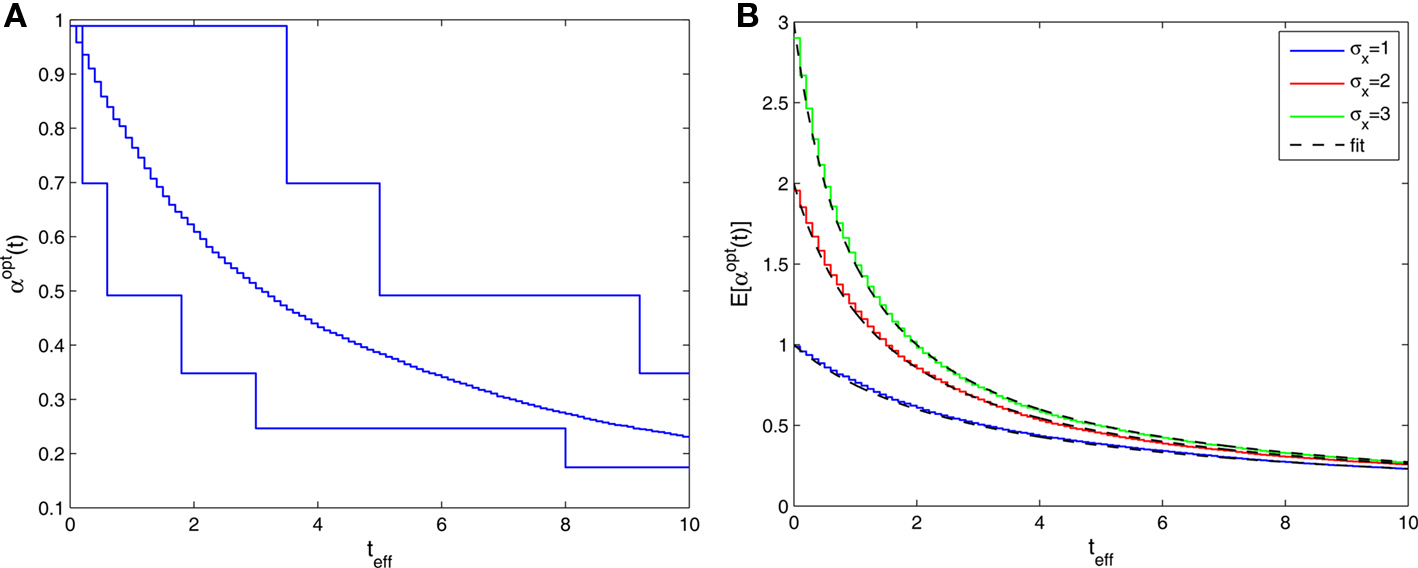
Figure 5. (A) Sample realizations of optimal width processes for fast (bottom) and slow (top) spiking processes. The average over 1000 trials is plotted in the middle (σ_x = 1 and Δt_eff = 0.1). (B) Average optimal width processes for different values of prior standard deviation, all coinciding with the function

When we examine the average optimal width process for different values of prior standard deviation (Figure 5B), we see that prior to the encoding onset it is always best to keep the tuning functions practically as wide as the probability density function of the stimulus (i.e., at t = 0, before any spikes are obtained, set α^opt (t = 0) = σ_x for all realizations). The average rate of dynamic narrowing is then related to the initial uncertainty, where the fastest narrowing occurs in the most uncertain environment. Note that under the conditions stated in Section “Analytical Derivation of the MMSE”, the mean population activity Σ_mλ_m(x) is proportional to the width parameter α. Thus, Figure 5B can be interpreted as reflecting a dynamic decrease in population activity as a function of time. Furthermore, there is an excellent empirical fit between the average optimal process to the simple function

Implementation of an optimal width process seems biologically implausible, due to its discontinuity and its perfect synchronization with the spikes. It is more likely for biological tuning functions to adopt the average optimal width process strategy, namely to automatically commence a dynamic narrowing at the beginning of an encoding period, independently of the generated spikes. But is the average optimal width process still more efficient than constant width? To address this question, we simulated the dynamics of four populations: two with constant widths tuned for optimal performance at the middle and at the end of the decoding time window, respectively, one with a piecewise-optimal width process and another one with a width function corresponding to the average optimal width process. As expected, each of the constant-width populations outperforms the other at the time for which it is tuned (Figure 6). The dynamic-width populations significantly outperform them both for short times, where for later times the differences become negligible. Therefore, implementation of dynamic width offers a clear advantage over operation with constant width, especially since there is seldom a reference time of interest to which the tuning functions could be tuned in advance. Interestingly, the predetermined width function is as good as the optimal width process for short times and even outperforms it for longer times, meaning that the performance is not being compromised when a predetermined width function is employed in place of the optimal width process.

FIGURE 6

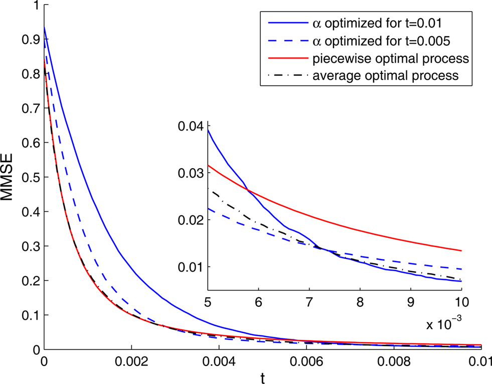
Figure 6. The MMSE associated with four different populations, each one tuned to a different optimality criterion. The MMSE was assessed using Monte Carlo methods. Inset: Enlargement for late times.

Biological implications

Our prediction that tuning functions should dynamically narrow during the course of encoding a stimulus, coincides with some reported experimental phenomena. Wang et al. (2005) recorded the activity of auditory cortical neurons in awake marmoset monkeys in response to a sound stimulus, which is the preferred stimulus of only one of the neurons. When comparing the activity profiles of the two neurons, they found that both fire intensively immediately following stimulus presentation, but only the neuron which is tuned to the stimulus maintained high activity throughout stimulus duration. Such behavior is equivalent to (and can stem from) dynamic narrowing of receptive fields. Widespread onset responses (caused by initially large receptive fields) subserve fast detection of the occurrence of sounds, whereas sustained firing in specific neurons facilitates extraction of the exact features of the sound. Dynamic narrowing of receptive fields following stimulus application was also observed in area 17 of anesthetized cats by Wörgötter et al. (1998). In the context of one-dimensional tuning functions, an illustrative example for dynamic narrowing was observed by Gutfreund et al. (2002) in the external nucleus of the inferior colliculus in anesthetized barn owls. The authors recorded from a population of neurons tuned to a short range of inter-aural time differences (ITD) in response to stimuli with different ITD values. While initial responses were intensive for all stimuli, intensive ongoing responses were restricted to stimuli within the ITD range preferred by the population, implying a dynamic reduction in tuning function width. A similar phenomenon was also obtained for single neurons. Benucci et al. (2009) quantified the instantaneous tuning functions of direction-sensitive V1 neurons in anesthetized cats and observed a dynamic narrowing following stimulus application, accompanied by a later recovery of the tuning function width, after the stimulus was changed or removed.

Discussion

In this paper we have studied optimal encoding of environmental signals by a population of spiking neurons, characterized by tuning functions which quantify the firing probability as a function of the input. Within the framework of optimal Bayesian decoding, based on the mean square reconstruction error criterion, we investigated the properties of optimal encoding. Based on the well known inequality, bounding the MMSE by the Bayesian Cramér–Rao lower bound (Eq. 6), we tested the hypothesis that the tuning function width minimizing the MMSE can be recovered by minimizing the lower bound. This hidden assumption was implied in previous studies dealing with classical, non-Bayesian, estimators based on neural decoding (Seung and Sompolinsky, 1993; Zhang and Sejnowski, 1999; Brown and Bäcker, 2006). Unfortunately, as argued in Section “Results”, the predictions were often incompatible with the assumptions required in the derivation of the bound, and thus could not be utilized to compare bound-based predictions with results based on direct minimization of the MMSE. It should be noted that in the non-Bayesian setting an optimal estimator does not necessarily exist, because the performance of each estimator depends on the stimulus, which is an unknown parameter. For instance, is the optimal estimator if and only if X = a. The above-mentioned studies overcame this problem by assuming that the tuning functions are dense enough so that the population’s Fisher information can be approximated by an integral and thus becomes independent of the stimulus. They all concluded that in one dimension estimation performance improves with narrower tuning curves. However, the underlying assumption is valid only when the width is large enough with respect to Δc, and obviously breaks down as α → 0. Therefore, values in the proximity of α = 0 are not part of the solution space, and lim_α→0𝒥(X) cannot be estimated using the suggested approximation. Moreover, realistic environments are dynamic and it seems more reasonable to model their features as random variables rather than unknown parameters. This means that optimal tuning curves may be more fruitfully examined within a Bayesian framework. Indeed, neurobiological evidence indicates that the nervous system can adapt to changes in the statistical nature of the environment and its random features at multiple time scales (e.g., Pettet and Gilbert, 1992; Brenner et al., 2000; Dragoi et al., 2000; Dean et al., 2005; Hosoya et al., 2005).

Starting from the Bayesian Cramér–Rao lower bound (Eq. 6) we have studied predictions about tuning function properties based on this bound which, under appropriate conditions, is asymptotically tight. As we demonstrated, this bound-based approach has little value in predicting the true optimal tuning functions for finite decoding time. Even though the performance inequalities hold in all scenarios, optimizing the bound does not guarantee the same behavior for the bounded quantity. Moreover, an important, and often overlooked observation is the following. Performance bounds might be too model-dependent, and when the model is misspecified (as is often the case) they lose their operative meaning. For instance, when the model is incorrect, the error does not converge asymptotically to the BCRB, even though the estimator itself might converge to the true value of the state (White, 1982). Thus, given that models are often inaccurate, the danger of using bounds is apparent even in the asymptotic limit.

By deriving analytical expressions for the minimal attainable MSE under various scenarios we have obtained optimal widths directly by minimizing the MMSE, without relying on bounds. Our analysis uncovers the dependence of optimal width on decoding time window, prior standard deviation and environmental noise. The relation between optimal width and prior standard deviation may very well explain physiological responses induced by attention, as noted in Section “MMSE-Based Optimal Width”, where further experimental evidence supporting the predictions of this paper was discussed. In particular, the work of Korte and Rauschecker (1993) related to tuning functions in the auditory cortex of cats with early blindness was discussed, and specific predictions were made. We also showed that when the constant-width restriction is removed, tuning functions should narrow during the course of encoding a stimulus, a phenomenon which has already been demonstrated for A1 neurons in marmoset monkeys (Wang et al., 2005) and in the external nucleus of the inferior colliculus in barn owls (e.g., Gutfreund et al., 2002).

In summary, in this paper we examined optimal neuronal tuning functions within a Bayesian setting based on the MMSE criterion. Careful calculations were followed by theoretical results, based on a natural criterion of optimality which is commonly employed, but which has seldom been analyzed in the context of neural encoding. Our analysis yielded novel predictions about the context-dependence of optimal widths, stating that optimal tuning curves should adapt to the statistical properties of the environment – in accordance with ecological theories of sensory processing. Interestingly, the results predict at least two time scales of change. For example, when the statistical properties of the environment change (e.g., a change in the noise level or prior distribution) the optimal encoding should adapt on the environmental time scale in such a way that the tuning function widths increases with noise level. However, even in the context of a fixed stimulus, we predict that tuning functions should change on the fast time scale of stimulus presentation. Interestingly, recent results, summarized by Gollisch and Meister (2010), consider contrast adaptation in the retina taking place on a fast and slow time scale (see also Baccus and Meister, 2002). The fast time scale, related to “contrast gain control” occurs on time scales of tens of millisecond, while the slow time-scale, lasting many seconds, has been referred to as “contrast adaptation”. While our results do not directly relate to contrast adaptation, the prediction that optimal adaptation takes place on at least two, widely separated, time scales is promising. Moreover, the circuit mechanisms proposed in (Gollisch and Meister, 2010) may well subserve some of the computations related to tuning function narrowing. These results, and the above-mentioned experimentally observed phenomena, suggest that biological sensory systems indeed adapt to changes in environmental statistics on multiple time scales. The theory provided in this paper offers a clear functional explanation of these phenomena, based on the notion of optimal dynamic encoding.

Conflict of Interest Statement

The authors declare that the research was conducted in the absence of any commercial or financial relationships that could be construed as a potential conflict of interest.

Acknowledgments

This work was partially supported by grant No. 665/08 from the Israel Science Foundation. We thank Eli Nelken and Yoram Gutfreund for helpful discussions.

References

Anderson, J., Lampl, I., Gillespie, D., and Ferster, D. (2000). The contribution of noise to contrast invariance of orientation tuning in cat visual cortex. Science 290, 1968–1972.

Pubmed Abstract | Pubmed Full Text | CrossRef Full Text

Averbeck, B., Latham, P., and Pouget, A. (2006). Neural correlations, population coding and computation. Nat. Rev. Neurosci. 7, 358–366.

Pubmed Abstract | Pubmed Full Text | CrossRef Full Text

Baccus, S., and Meister, M. (2002). Fast and slow contrast adaptation in retinal circuitry. Neuron 36, 909–919.

Pubmed Abstract | Pubmed Full Text | CrossRef Full Text

Barbieri, R., Frank, L., Nguyen, D., Quirk, M., Solo, V., Wilson, M., and Brown, E. (2004). Dynamic analyses of information encoding in neural ensembles. Neural Comput. 16, 277–307.

Pubmed Abstract | Pubmed Full Text | CrossRef Full Text

Beck, J., Ma, W., Kiani, R., Hanks, T., Churchland, A., Roitman, J., Shadlen, M., Latham, P., and Pouget, A. (2008). Probabilistic population codes for Bayesian decision making. Neuron 60, 1142–1152.

Pubmed Abstract | Pubmed Full Text | CrossRef Full Text

Beck, J., and Pouget, A. (2007). Exact inferences in a neural implementation of a hidden Markov model. Neural Comput. 19, 1344–1361.

Pubmed Abstract | Pubmed Full Text | CrossRef Full Text

Benucci, A., Ringach, D., and Carandini, M. (2009). Coding of stimulus sequences by population responses in visual cortex. Nat. Neurosci. 12, 1317.

Pubmed Abstract | Pubmed Full Text | CrossRef Full Text

Bethge, M., Rotermund, D., and Pawelzik, K. (2002). Optimal short-term population coding: when Fisher information fails. Neural Comput. 14, 2317–2351.

Pubmed Abstract | Pubmed Full Text | CrossRef Full Text

Bethge, M., Rotermund, D., and Pawelzik, K. (2003). Optimal neural rate coding leads to bimodal firing rate distributions. Netw. Comput. Neural Syst. 14, 303–319.

CrossRef Full Text

Bobrowski, O., Meir, R., and Eldar, Y. (2009). Bayesian filtering in spiking neural networks: noise, adaptation, and multisensory integration. Neural Comput. 21, 1277–1320.

Pubmed Abstract | Pubmed Full Text | CrossRef Full Text

Brenner, N., Bialek, W., and de Ruyter van Steveninck, R. (2000). Adaptive rescaling maximizes information transmission. Neuron 26, 695–702.

Pubmed Abstract | Pubmed Full Text | CrossRef Full Text

Brown, W., and Bäcker, A. (2006). Optimal neuronal tuning for finite stimulus spaces. Neural Comput. 18, 1511–1526.

Pubmed Abstract | Pubmed Full Text | CrossRef Full Text

Brunel, N., and Nadal, J. (1998). Mutual information, Fisher information, and population coding. Neural Comput. 10, 1731–1757.

Pubmed Abstract | Pubmed Full Text | CrossRef Full Text

Dean, I., Harper, N., and McAlpine, D. (2005). Neural population coding of sound level adapts to stimulus statistics. Nat. Neurosci. 8, 1684–1689.

Pubmed Abstract | Pubmed Full Text | CrossRef Full Text

Dean, I., Robinson, B., Harper, N., and McAlpine, D. (2008). Rapid neural adaptation to sound level statistics. J. Neurosci. 28, 6430–6438.

Pubmed Abstract | Pubmed Full Text | CrossRef Full Text

Deneve, S. (2008). Bayesian spiking neurons I: inference. Neural Comput. 20, 91–117.

Pubmed Abstract | Pubmed Full Text | CrossRef Full Text

Deneve, S., Latham, P., and Pouget, A. (2001). Efficient computation and cue integration with noisy population codes. Nat. Neurosci. 4, 826–831.

Pubmed Abstract | Pubmed Full Text | CrossRef Full Text

Dragoi, V., Sharma, J., and Sur, M. (2000). Adaptation-induced plasticity of orientation tuning in adult visual cortex. Neuron 28, 287–298.

Pubmed Abstract | Pubmed Full Text | CrossRef Full Text

Duncan, T. (1970). On the calculation of mutual information. SIAM J. Appl. Math. 19, 215–220.

CrossRef Full Text

Eden, U., Frank, L., Barbieri, R., Solo, V., and Brown, E. (2004). Dynamic analysis of neural encoding by point process adaptive filtering. Neural Comput. 16, 971–998.

Pubmed Abstract | Pubmed Full Text | CrossRef Full Text

Ernst, M., and Banks, M. (2002). Humans integrate visual and haptic information in a statistically optimal fashion. Nature 415, 429–433.

Pubmed Abstract | Pubmed Full Text | CrossRef Full Text

Eurich, C., Wilke, S., and Schwegler, H. (2000). Neural representation of multi-dimensional stimuli. Adv. Neural Inf. Process Syst. 12, 115–121.

Finney, E., Fine, I., and Dobkins, K. (2001). Visual stimuli activate auditory cortex in the deaf. Nat. Neurosci. 4, 1171–1174.

Pubmed Abstract | Pubmed Full Text | CrossRef Full Text

Geisler, W., Najemnik, J., and Ing, A. (2009). Optimal stimulus encoders for natural tasks. J. Vision 9, 13–17.

CrossRef Full Text

Gollisch, T., and Meister, M. (2010). Eye smarter than scientists believed: neural computations in circuits of the retina. Neuron 65, 150–164.

Pubmed Abstract | Pubmed Full Text | CrossRef Full Text

Guo, D., Shamai, S., and Verdú, S. (2005). Mutual information and minimum mean-square error in Gaussian channels. IEEE Trans. Inf. Theory 51, 1261–1282.

CrossRef Full Text

Gutfreund, Y., Zheng, W., and Knudsen, E. (2002). Gated visual input to the central auditory system. Science 297, 1556.

Pubmed Abstract | Pubmed Full Text | CrossRef Full Text

Harper, N., and McAlpine, D. (2004). Optimal neural population coding of an auditory spatial cue. Nature 430, 682–686.

Pubmed Abstract | Pubmed Full Text | CrossRef Full Text

Hosoya, T., Baccus, S., and Meister, M. (2005). Dynamic predictive coding by the retina. Nature 436, 71–77.

Pubmed Abstract | Pubmed Full Text | CrossRef Full Text

Huys, Q., Zemel, R., Natarajan, R., and Dayan, P. (2007). Fast population coding. Neural Comput. 19, 404–441.

Pubmed Abstract | Pubmed Full Text | CrossRef Full Text

Jacobs, A., Fridman, G., Douglas, R., Alam, N., Latham, P., Prusky, G., and Nirenberg, S. (2009). Ruling out and ruling in neural codes. Proc. Natl. Acad. Sci. U.S.A. 106, 5936–5941.

Pubmed Abstract | Pubmed Full Text | CrossRef Full Text

Jacobs, R. (1999). Optimal integration of texture and motion cues to depth. Vision Res. 39, 3621–3629.

Pubmed Abstract | Pubmed Full Text | CrossRef Full Text

Johnson, D., and Ray, W. (2004). Optimal stimulus coding by neural populations using rate codes. J. Comput. Neurosci. 16, 129–138.

Pubmed Abstract | Pubmed Full Text | CrossRef Full Text

Knill, D., and Pouget, A. (2004). The Bayesian brain: the role of uncertainty in neural coding and computation. Trends Neurosci. 27, 712–719.

Pubmed Abstract | Pubmed Full Text | CrossRef Full Text

Knill, D., and Richards, W. (1996). Perception as Bayesian Inference. New York, NY: Cambridge University Press.

Korte, M., and Rauschecker, J. (1993). Auditory spatial tuning of cortical neurons is sharpened in cats with early blindness. J. Neurophysiol. 70, 1717.

Pubmed Abstract | Pubmed Full Text

Lánskỳ, P., and Greenwood, P. (2005). Optimal signal estimation in neuronal models. Neural Comput. 17, 2240–2257.

CrossRef Full Text

Liu, Y., Stevens, C., and Sharpee, T. (2009). Predictable irregularities in retinal receptive fields. Proc. Natl. Acad. Sci. U.S.A. 106, 16499–16504.

Pubmed Abstract | Pubmed Full Text | CrossRef Full Text

Marom, S., Meir, R., Braun, E., Gal, A., Kermany, E., and Eytan, D. (2009). On the precarious path of reverse neuro-engineering. Front. Comput. Neurosci. 3:5. doi: 10.3389/neuro.10.005.2009.

Pubmed Abstract | Pubmed Full Text | CrossRef Full Text

Martinez-Trujillo, J., and Treue, S. (2004). Feature-based attention increases the selectivity of population responses in primate visual cortex. Curr. Biol. 14, 744–751.

Pubmed Abstract | Pubmed Full Text | CrossRef Full Text

Ma, W., Beck, J., Latham, P., and Pouget, A. (2006). Bayesian inference with probabilistic population codes. Nat. Neurosci. 9, 1432–1438.

Pubmed Abstract | Pubmed Full Text | CrossRef Full Text

McDonnell, M., and Stocks, N. (2008). Maximally informative stimuli and tuning curves for sigmoidal rate-coding neurons and populations. Phys. Rev. Lett. 101, 058103.

Pubmed Abstract | Pubmed Full Text | CrossRef Full Text

Nikitin, A., Stocks, N., Morse, R., and McDonnell, M. (2009). Neural population coding is optimized by discrete tuning curves. Phys. Rev. Lett. 103, 138101.

Pubmed Abstract | Pubmed Full Text | CrossRef Full Text

Panzeri, S., Treves, A., Schultz, S., and Rolls, E. (1999). On decoding the responses of a population of neurons from short time windows. Neural Comput. 11, 1553–1577.

Pubmed Abstract | Pubmed Full Text | CrossRef Full Text

Pettet, M., and Gilbert, C. (1992). Dynamic changes in receptive-field size in cat primary visual cortex. Proc. Natl. Acad. Sci. U.S.A. 89, 8366–8370.

Pubmed Abstract | Pubmed Full Text | CrossRef Full Text

Pitkow, X., Sompolinsky, H., and Meister, M. (2007). A neural computation for visual acuity in the presence of eye movements. PLoS Biol. 5, e331. doi: 10.1371/journal.pbio.0050331.

Pubmed Abstract | Pubmed Full Text | CrossRef Full Text

Pouget, A., Dayan, P., and Zemel, R. (2000). Information processing with population codes. Nat. Rev. Neurosci. 1, 125–132.

Pubmed Abstract | Pubmed Full Text | CrossRef Full Text

Pouget, A., Dayan, P., and Zemel, R. (2003). Computation and inference with population codes. Annu. Rev. Neurosci. 26, 381–410.

Pubmed Abstract | Pubmed Full Text | CrossRef Full Text

Pouget, A., Deneve, S., Ducom, J., and Latham, P. (1999). Narrow versus wide tuning curves: what’s best for a population code? Neural Comput. 11, 85–90.

Pubmed Abstract | Pubmed Full Text | CrossRef Full Text

Pouget, A., Deneve, S., and Duhamel, J. (2002). A computational perspective on the neural basis of multisensory spatial representations. Nat. Rev. Neurosci. 3, 741–747.

Pubmed Abstract | Pubmed Full Text | CrossRef Full Text

Rao, R. (2004). Bayesian computation in recurrent neural circuits. Neural Comput. 16, 1–38.

Pubmed Abstract | Pubmed Full Text | CrossRef Full Text

Rauschecker, J., and Harris, L. (1983). Auditory compensation of the effects of visual deprivation in the cat’s superior colliculus. Exp. Brain Res. 50, 69–83.

Pubmed Abstract | Pubmed Full Text | CrossRef Full Text

Searle, S. (1982). Matrix Algebra Useful for Statistics. New York, NY: John Wiley & Sons.

Seriès, P., Latham, P., and Pouget, A. (2004). Tuning curve sharpening for orientation selectivity: coding efficiency and the impact of correlations. Nat. Neurosci. 7, 1129–1135.

CrossRef Full Text

Seung, H., and Sompolinsky, H. (1993). Simple models for reading neuronal population codes. Proc. Natl. Acad. Sci. U.S.A. 90, 10749–10753.

Pubmed Abstract | Pubmed Full Text | CrossRef Full Text

Toyoizumi, T., Aihara, K., and Amari, S. (2006). Fisher information for spike-based population decoding. Phys. Rev. Lett. 97, 098102.

Pubmed Abstract | Pubmed Full Text | CrossRef Full Text

Twum-Danso, N., and Brockett, R. (2001). Trajectory estimation from place cell data. Neural Netw. 14, 835–844.

Pubmed Abstract | Pubmed Full Text | CrossRef Full Text

Van Trees, H. (1968). Detection, Estimation, and Modulation Theory, Part I. New York, NY: John Wiley & Sons.

Van Trees, H., and Bell, K. (2007). Bayesian Bounds for Parameter Estimation and Nonlinear Filtering/Tracking. New York, NY: John Wiley & Sons.

Wang, X., Lu, T., Snider, R., and Liang, L. (2005). Sustained firing in auditory cortex evoked by preferred stimuli. Nature 435, 341.

Pubmed Abstract | Pubmed Full Text | CrossRef Full Text

Weeks, R., Horwitz, B., Aziz-Sultan, A., Tian, B., Wessinger, C., Cohen, L., Hallett, M., and Rauschecker, J. (2000). A positron emission tomographic study of auditory localization in the congenitally blind. J. Neurosci. 20, 2664.

Pubmed Abstract | Pubmed Full Text

White, H. (1982). Maximum likelihood estimation of misspecified models. Econometrica 50, 1–25.

CrossRef Full Text

Wörgötter, F., Suder, K., Zhao, Y., Kerscher, N., Eysel, U., and Funke, K. (1998). State-dependent receptive field restructuring in the visual cortex. Nature 396, 165–168.

Pubmed Abstract | Pubmed Full Text | CrossRef Full Text

Yeshurun, Y., and Carrasco, M. (1999). Spatial attention improves performance in spatial resolution tasks. Vision Res. 39, 293–306.

Pubmed Abstract | Pubmed Full Text | CrossRef Full Text

Zemel, R., Dayan, P., and Pouget, A. (1998). Probabilistic interpretation of population codes. Neural Comput. 10, 403–430.

Pubmed Abstract | Pubmed Full Text | CrossRef Full Text

Zhang, K., and Sejnowski, T. (1999). Neuronal tuning: to sharpen or broaden? Neural Comput. 11, 75–84.

Pubmed Abstract | Pubmed Full Text | CrossRef Full Text