Enabling functional neural circuit simulations with distributed computing of neuromodulated plasticity

1 Introduction

It is generally assumed that mammalian learning is implemented by changes in synaptic efficacy, as it is the case in simpler organisms (see e.g., Antonov et al., 2003). Historically, attempts to provide a theoretical explanation of learning have mainly been influenced by Hebb’s postulate (Hebb, 1949) that the sequential activation of two neurons strengthens the synapse connecting them. Thus, theoretical “Hebbian” plasticity rules depend on the pre- and post-synaptic activity and sometimes also on the weight itself. Although these rules have been shown to solve some interesting problems (Gerstner et al., 1996; Song et al., 2000; Song and Abbott, 2001) it is not clear that such “two factor” rules can be the mechanism that enables animals to learn complicated tasks, such as those to find sparse rewards in complex environments.

However, experiments have shown that in some preparations, synaptic plasticity depends not only on the activity of the pre- and post-synaptic neurons but also on the presence of neuromodulators such as acetylcholine, norepinephrine, serotonin, and dopamine. Neuromodulators are released from neurons that are primarily located in the brainstem and basal forebrain, but that innervate many brain areas through long range connections (for a review see Cooper et al., 2002). The functional consequences of the long-range neuromodulatory projections are very diverse and depend strongly on the specific neuromodulator, the target area and the neuromodulatory concentration. For example, the release of acetylcholine from the basal forebrain into the cortex is involved in the control of attention (Hasselmo and McGaughy, 2004; Herrero et al., 2008; Deco and Thiele, 2009), and noradrenaline, mainly originating from the locus coeruleus, is released throughout the central nervous system facilitating the processing of relevant, or salient, information (Berridge and Waterhouse, 2003). One neuromodulatory function which has evoked high interest in the experimental as well as the theoretical neuroscience communities is reward learning on the basis of dopamine released in the striatum from midbrain areas (Schultz et al., 1997; Reynolds et al., 2001).

An influential hypothesis on the mechanism of neuromodulation is that neuromodulators can be released extrasynaptically from en passant boutons on neuromodulatory axons and modulate the plasticity of synapses that are remote from release sites, a concept known as volume transmission (Agnati et al., 1995; Zoli and Agnati, 1996). This is illustrated in Figure 1. For an illustration of en passant boutons on a neuromodulatory axon and a schematic representation of the main sources of volume transmission signals, see Moreau et al. (2010) and Zoli et al. (1999), respectively. This hypothesis implies a temporal rather than a spatial selectivity for neuromodulatory action (Arbuthnott and Wickens, 2007). Pawlak et al. (2010) in this special issue review the recent experimental in vitro findings concerning the effects of neuromodulators released from long-range neuromodulatory systems on STDP. Despite the large range of time scales and the variety of mechanisms by which the neuromodulators influence STDP, the review finds that the effects can be divided into two categories. In the first category, the neuromodulator is essentially required for the induction of STDP. In the second category, the neuromodulator alters the threshold for the plasticity induction. The review argues that the neuromodulatory influence is the crucial mechanism linking synaptic plasticity to behaviorally based learning, especially when learning depends on a reward signal. This hypothesis is further supported by a number of spiking neuronal network models that can learn a reward related task, due to the incorporation of three-factor synaptic plasticity rules (Seung, 2003; Xie and Seung, 2004; Baras and Meir, 2007; Florian, 2007; Izhikevich, 2007; Legenstein et al., 2008; Potjans et al., 2009b; Vasilaki et al., 2009).

FIGURE 1

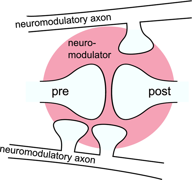
Figure 1. Volume transmission: a neuromodulator is released from en passant boutons on neuromodulatory axons and modulates the plasticity of synapses remote from the release sites as a “third factor. ” The modulatory signal is a composition of the neuromodulator released by multiple boutons in a certain area (three are shown). For simplicity the figure shows only one modulated synapse. However, commonly the signal is assumed to affect multiple synapses within a certain volume (pink area).

These spiking neuronal network models of reward learning are typically formulated in a general way before being tested in concrete tasks. The generation of the neuromodulatory signal, or third factor, is determined by the task to be solved. Three categories can be identified for the generation of the neuromodulatory signal: either the signal is injected into the spiking network by an external controller, or it is determined by a mixture of an external supervisor and the spiking activity of the network or it is generated purely internally. The categories can be further discriminated with respect to the points in time leading to discontinuous changes in the value of the signal. An update can be triggered by an external event (such as an external stimulus), by the generation of a spike or it can be driven in discrete time steps. The neuromodulatory signal is either represented as a discrete variable that has a non-zero value only at the points in time that an update is triggered, or it is represented as a continuous variable between discontinuous updates. The three categories and their sub-categories are illustrated in Figure 2.

FIGURE 2

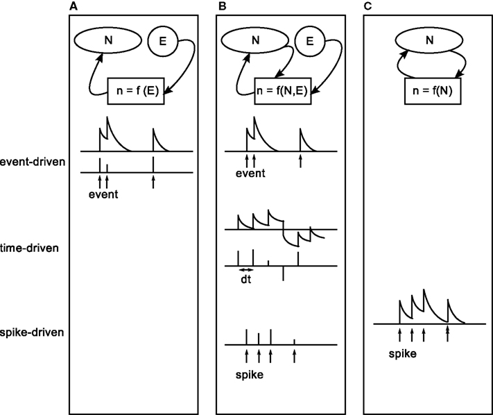
Figure 2. Characterization of existing modeling studies with respect to the generation process of a plasticity modulating signal. From left to right: interplay between external (E) and internal (N) information in the generation process of the modulatory signal (n). (A) The signal is generated purely externally (task two in Izhikevich, 2007; Potjans et al., 2009b; Vasilaki et al., 2009). (B) The signal combines information from an external supervisor and internal information (Seung, 2003; Xie and Seung, 2004; Baras and Meir, 2007; Florian, 2007; Izhikevich, 2007, task three). (C) The signal is generated purely internally (task four in Izhikevich, 2007; Legenstein et al., 2008). From top to bottom: timing of discontinuous updates to the signal. Top: updates are triggered by external events, indicated by arrows (event-driven). Middle: updates occur in discrete time steps dt (time-driven). Bottom: updates triggered by the arrival of neuromodulatory spikes, indicated by arrows (spike-driven). Upper and lower rows show a signal that takes continuous values between updates, or discrete values at the times of updates, respectively.

In the first category (Figure 2A), the plasticity modulating signal does not depend on the spiking activity of the network at all. The signal is updated in an event-driven fashion triggered by external events, such as entering a reward-related state in a navigation task or the occurrence of a reward predicting stimulus in classical conditioning tasks. Both discrete-time (Potjans et al., 2009b; Vasilaki et al., 2009) and continuous-time (task two in Izhikevich, 2007) representations of the neuromodulatory signal have been investigated.

In the second category (Figure 2B), the generation of the plasticity modulating signal requires the presence of an all-knowing external supervisor. The signal depends on the interplay between information provided externally and internally. Signal updates are triggered by the occurrence of an external event (task three in Izhikevich, 2007) or the emission of a spike of a specific output neuron within the network (XOR task in Florian, 2007; Seung, 2003; Xie and Seung, 2004); alternatively, the signal is generated in discrete time steps (Baras and Meir, 2007, target firing learning model in Florian, 2007). In the event-driven model proposed by Izhikevich (2007) to solve an instrumental conditioning task, the signal is modeled as a continuous variable where the timing and magnitude of updates are determined externally. Whether the update is actually carried out by the synapses is contingent on an internal condition (i.e., a comparison of firing rates in two pools) meeting an externally imposed criterion (i.e., the desired ordering of the firing rates). In the models proposed by Seung (2003), Xie and Seung (2004), and Florian (2007) to solve a XOR task, updates are triggered by the spikes of an output neuron; the magnitudes of the updates are determined by an external supervisor that evaluates the response of the output neuron to the spiking activity of an input layer representing different combinations of 0 and 1. For an input of [0,1] or [1,0], every spike of the output neuron results in a positive value for the neuromodulatory signal, whereas a negative value is generated for each input spike in response to an input of [0,0] or [1,1]. Between spikes of the output neuron, the value of the neuromodulatory signal is zero.

Other models in the second category assume that the signal is updated in discrete-time steps in n·ΔT, where n is an integer; ΔT can be a small step size or the duration of a certain episode. This is illustrated in the middle row of Figure 2B. Here the values of the signal are determined as a function of the spiking activity in comparison to a desired activity which is provided by an external supervisor. The signal can either take continuous values, as in the model proposed by Baras and Meir (2007) to solve a path learning task and the target firing-rate learning model proposed by Florian (2007) or discrete values at specific times, as in an alternative variant of the target firing-rate learning model proposed by Florian (2007) and the XOR learning model proposed by Baras and Meir (2007).

The first two categories demonstrate the importance of three-factor rules in solving reward related tasks of different complexity, ranging from XOR to navigation tasks. However, in order to understand how different brain areas interact to produce cognitive functions these models are not sufficient. This problem requires the consideration of functionally closed loop models, where the neuromodulatory signal is generated by the network itself (Figure 2C). So far, only two studies have investigated such models. In both the model proposed by Izhikevich (2007), which learns a shift in dopamine response from an unconditional stimulus to a reward-predicting conditional stimulus, and that proposed by Legenstein et al. (2008) which learns a biofeedback task, each spike of a specific population of neurons leads to an update of a continuous-time variable.

The simulation of models in this third category and the spike-based models of the second category is beset by considerable technical challenges. Spike-driven updates are intrinsically more troublesome than updates driven by external events or occurring in regular intervals, as they do not entail a natural interruption point for the simulation at which signal information can be calculated and conveyed to the relevant synapses. This difficulty is compounded in the context of models where different brain regions interact, as the neuromodulatory signal is not only likely to be composed of the activity of a population of neurons, but also affecting synapses between entirely different populations. A final hurdle comes with model size. The spiking network models implementing three-factor synaptic plasticity rules discussed above consist only of a small (of the order of 10 to 10²) (Seung, 2003; Xie and Seung, 2004; Baras and Meir, 2007; Florian, 2007; Potjans et al., 2009b; Vasilaki et al., 2009) to moderate (of the order of 10³) number of neurons (Izhikevich, 2007; Legenstein et al., 2008). However, to simultaneously achieve cortical levels of connectivity (10%) and number of inputs (10⁴) (Braitenberg and Schüz, 1998), a minimal network size of 10⁵ neurons is required. Similarly, to investigate brain-scale circuits involving the interaction of multiple brain areas, large-scale networks are likely to be necessary. Consequently, distributed computing techniques are required. Indeed, even the systematic study of smaller networks demand such techniques as learning often takes place on a very long time scale compared to the time scale of synaptic plasticity. The requirement for distributed computing adds to the complexity of the problem of implementing neuromodulated plasticity via volume transmission. The challenge can be stated as follows: how can a synapse, which is typically only accessed through its pre-synaptic neuron, be efficiently informed about a neuromodulatory signal generated by a population of neurons that are generally located on machines different than those of either the pre- or the postsynaptic neuron. Whereas efficient methods exist to integrate the dynamics of large-scale models by distributed computing (Hammarlund and Ekeberg, 1998; Harris et al., 2003; Morrison et al., 2005), so far no solution for the efficient implementation of neuromodulated plasticity in spiking neuronal networks has been presented. Studies of network models in which the neuromodulatory signal is internally generated have not provided any technical details (Izhikevich, 2007; Legenstein et al., 2008), thus the models cannot be reproduced or extended by the wider modeling community.

To address this gap and thus open up this fascinating area of research, we present a framework for the implementation of neuromodulated plasticity in time-driven simulators operating in a distributed environment. The framework is general, in that it is suitable for all manner of simulations rather than one specific network model or task. Moreover, we do not focus on a specific implementation language, neuromodulator or neuromodulated plasticity mechanism and rely on only a few assumptions about the infrastructure of the underlying simulator. In the framework the plasticity modulating signal is generated by a user-defined population of neurons contained within the network. The neuromodulatory signal influences all synapses located in a user-defined specific volume, modeling the effect of volume transmission (see Figure 1). Our framework yields excellent scaling for recurrent networks incorporating neuromodulated STDP in its excitatory to excitatory connections. In order to analyze the efficiency of the framework implementation accurately, we develop a general technique to decompose the total run time into the portion consumed by communication between machines and the portion consumed by computation. This separation enables us to distinguish the saturation in run time caused by communication overhead from any potential saturation caused by a sub-optimal algorithm design. This technique can be applied to arbitrary network simulations und will thus aid the future development and analysis of extensions to distributed simulation tools.

A general scheme for the distributed simulation of neural networks is summarized in section 2.1 to clarify terminology and make explicit the assumptions made about the simulator infrastructure. In section 3.1 we present an efficient way to implement neuromodulated plasticity in this distributed simulation environment. To illustrate the technique, in section 3.2 we compare the run times of recurrent networks (10⁴ and 10⁵ neurons) incorporating neuromodulated spike-timing dependent plasticity (Izhikevich, 2007) to those of networks incorporating the corresponding “two factor” spike-timing dependent plasticity.

The conceptual and algorithmic work described here is a module in our long-term collaborative project to provide the technology for neural systems simulations (Gewaltig and Diesmann, 2007). Preliminary results have been already presented in abstract form (Potjans et al., 2009a).

2 Materials and Methods

2.1 Distributed Neural Network Simulation

To clarify the terminology used in the rest of the manuscript and define the requirements a simulator must fulfill in order to incorporate our framework for neuromodulated plasticity, in the following we briefly describe a general purpose time-driven simulation scheme for distributed computation. For a more thorough and illustrated description, see Morrison et al. (2005). Variants of this scheme underlie the majority of simulators that are designed for simulating networks of point neurons, for example NEST (Gewaltig and Diesmann, 2007), C2 (Ananthanarayanan and Modha, 2007) and PCSIM (Pecevski et al., 2009), see Brette et al. (2007) for a review.

2.1.1 Network representation

Our fundamental assumption is that a neural network can be represented as a directed graph, consisting of nodes and the connections between them. The class of nodes comprises spiking neurons (either single- or few-compartment models) and devices, which are used to stimulate or record from neurons. A connection enables information to be sent from a sending node to a receiving node. The definition of a connection typically includes at least a weight and a delay. The weight determines the strength of a signal and the delay how long it takes for the signal to travel from the sending to the receiving node. The simplest synapse model delivers a fixed connection weight to the post-synaptic node. If the connection is intended to be plastic, the connection definition must also include a mechanism that defines the weight dynamics. “Two factor” rules, such as spike-timing dependent plasticity, can be implemented if the post-synaptic node maintains a history of its relevant state variables (e.g., as described in Morrison et al., 2007).

Each neuron is represented on exactly one of the m machines running the simulation, and synapses are distributed such that they are represented on the same machine as their post-synaptic target. Distributing the axon of a sending node in this way has a considerable advantage in communication costs compared to distributing dendrites (Morrison et al., 2005). In contrast to the neurons, each device is represented on every machine and only interacts with the local neurons. This reduces the communication load, as measured data or stimulation signals do not have to be transferred between machines. The cost of this approach is that m data files are generated for each recording device.

2.1.2 Simulation dynamics

Time-driven network update. The network is evaluated on an evenly spaced time grid t_i = i·Δt. At each grid point the network is in a well defined state S_i. The time interval Δt between two updates can be maximized by setting it to the minimal propagation delay d_min of the network. This is the largest permissible temporal desynchronization between any two nodes in the network (see Lamport, 1978; Morrison et al., 2005; Plesser et al., 2007). Note that the computation resolution for the neuron models can be much finer than the resolution of the global scheduling algorithm, for example neurons can advance their dynamics with a time step h = 0.1 ms even if the global algorithm advances in communication intervals of Δt = 1 ms. Alternatively, neuron model implementations can be defined within this framework that advance their dynamics in an event-driven fashion, i.e., from one incoming spike to the next (Morrison et al., 2007; Hanuschkin et al., 2010).

During a network update from one time step to the next, i.e., the interval (t_{i − 1},t_i], a global state transfer function U(S_i) propagates the network from one state S_i to the next S_i+1. As a result of this, each neuron may generate one or more spike events which are communicated to the other machines at the end of the update interval at t_i. Before the start of the next network update, i.e., the interval (t_i,t_i+1], the communicated events are delivered to their targets. This is described in greater detail below. In the following, we will refer to Δt as the communication interval. To implement our framework for neuromodulated plasticity, we therefore assume that the update cycle of the underlying simulator in a distributed environment can be expressed as the following algorithm:

1: T ←0
2: while T Tstop do
3:     parallel on all machines do
4:        deliver events received at last
            communication to targets
5:        call U(sT )
6:     end parallel
7:     communicate new events between machines
8:     increment network time: T ←T + Δt
9: end while

Event delivery. A neuron’s spike events must be delivered to its target nodes with a propagation delay determined by the connecting synapse. After the communication of events that takes place after each Δt interval, the simulation algorithm activates the outgoing synapses of the neurons that spiked during the previous interval. The sequence diagram for a simple synapse model is shown in Figure 3A. The synapse generates an event of weight w and delay d. The delay is determined by subtracting the lag between spike generation and communication from the propagation delay associated with the synapse: for a spike generated at s_pre and communicated at t_i with a total synaptic propagation delay d_syn, the remaining delay d is equal to d_syn - (t_i - s_pre). The event is sent to the synapse’s target node, which writes the event to its incoming event buffer such that it becomes visible to the update dynamics of the target neuron at the correct time step, s_pre + d_syn. A description of the ordering of buffer reading and writing operations to ensure that events are integrated correctly can be found in Morrison and Diesmann (2008). For the purposes of this manuscript, we assume that a simulator delivers events as described above, i.e., spikes have propagation delays, are communicated between machines at regular intervals and are buffered at the target neuron until they are due to be incorporated in the neuronal dynamics.

FIGURE 3

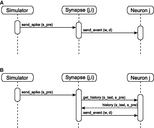
Figure 3. Sequence diagram for static (A) and STDP (B) synapses. The object Synapse (j,i) denotes a synapse from source neuron i to target neuron j; neuron i emits a spike at time s_pre.

Synapse update. In contrast to neurons, incoming events are rare for individual synapses at realistic firing rates. Therefore, to develop our framework we make the assumption that a simulator uses the more efficient strategy of updating synapses in an event-driven fashion only on the arrival of a pre-synaptic spike rather than in a time-driven fashion as neurons are. This is possible for the class of synaptic models that only depend on local factors such as the current weight of the synapse, the time since the last update and state information available from the post-synaptic neuron (Morrison et al., 2008). This class includes synaptic depression (Thomson and Deuchars, 1994), synaptic redistribution (Markram and Tsodyks, 1996) and spike-timing dependent plasticity (STDP) (Markram et al., 1997; Bi and Poo, 1998, 2001).

As we measure performance on the example of STDP with a neuromodulatory third factor (see section 3.2) it is worth discussing the infrastructure for calculating STDP updates triggered only on the arrival of pre-synaptic spikes in somewhat more detail. See Figure 3B for the sequence diagram for the activation of an STDP synapse; the corresponding pseudo-code is given in Morrison et al. (2007). All post-synaptic variables, such as the post-synaptic spike times and the low-pass filtered post-synaptic rate, are stored at the post-synaptic neuron. On the arrival of a pre-synaptic spike, the synapse requests these variables from the post-synaptic neuron for the period between the last and the current pre-synaptic spike (get_history(s_last,s_pre)). Based on this information the synapse can integrate its weight dynamics from one spike time to the next. The post-synaptic variables only have to be stored until they have been processed by every incoming synapse. After the weight has been updated an event is sent to the post-synaptic neuron as in the case of the simple synapse model discussed in section 2.1.2 and illustrated in Figure 3A.

2.2 Benchmark Network Models

To investigate the performance of our proposed framework, we measure the simulation times of recurrent networks incorporating neuromodulated spike-timing dependent plasticity at their excitatory–excitatory connections whilst systematically varying the number of processors used. The STDP model uses an all-to-all spike pairing scheme and is based on the model proposed by Izhikevich (2007):

where c is an eligibility trace, n the neuromodulator concentration, s_pre/post the time of a pre- or post-synaptic spike, s_n the time of a neuromodulatory spike, and C₁ and C₂ are constant coefficients. δ(t) is the Dirac delta function; τ_c and τ_n are the time constants of the eligibility trace and the neuromodulator concentration, respectively. Unlike the networks investigated by Izhikevich (2007), the neuromodulator concentration is always present, so we subtract a baseline b from the neuromodulator concentration. STDP(Δt) is the window function of additive STDP:

where Δt = s_post − s_pre is the temporal difference between a post-synaptic and a pre-synaptic spike, A₊ and A₋ are the amplitudes of the weight change and τ₊ and τ₋ are time constants. As a control, we also measure the simulation times of networks in which the neuromodulated STDP is exchanged for STDP without neuromodulation according to the model of Song and Abbott (2001), i.e., . In the neuromodulated and the unmodulated networks the synaptic weights are bounded between 0 and a maximal synaptic weight w_max.

We investigate the performance for networks of two different sizes: 1.125 × 10⁴ and 1.125 × 10⁵, referred to in the rest of the manuscript as the 10⁴ and 10⁵ networks, respectively. Both networks consist of 80% excitatory and 20% inhibitory current based integrate-and-fire neurons. In the subthreshold range the membrane potential V is determined by the following dynamics:

where τ_m is the membrane time constant, C_m the membrane capacity and I(t) the input current to the neuron, which is the sum of any external currents and the synaptic currents. The synaptic current I_syn due to an incoming spike is represented by an exponential function:

where w is the weight of the corresponding synapse and τ_syn the rise time. If the membrane potential passes the threshold V_th a spike is emitted and the neuron is clamped to the reset potential V_reset for the duration of the refractory period τ_ref.

The excitatory–excitatory connections are plastic, as described above; all other connections are static. All neurons receive additional Poissonian background noise. The network firing rate due to the Poissonian background noise of both networks is approximately 10 Hz in the asynchronous irregular regime. We arbitrarily choose the first N_nm excitatory neurons to be the neuromodulator releasing neurons. A tabular description of the benchmark network models and a specification of the parameters used can be found in Tables 1 and 2 of Appendix.

The simulations are carried out using the simulation tool NEST (Gewaltig and Diesmann, 2007) with a computation time step of 0.1 ms and a communication interval equal to the minimal propagation delay d_min. The simulations of the 10⁴ neuron networks are performed on a cluster of SUN X86 consisting of 23 compute nodes equipped with two AMD Opteron 2834 quad core processors with 2.7 GHz clock speed running Ubuntu Linux. The nodes are connected via InfiniBand (24 ports InfiniBand switch, Voltaire ISR9024D-M); the MPI implementation is OpenMPI 1.3.1. The simulations for the 10⁵ neuron networks are performed on a Bluegene/P (JUGENE¹).

3 Results

3.1 Implementing Neuromodulated Plasticity in a Distributed Environment

In this section we present a novel and general framework to implement neuromodulated plasticity efficiently for a distributed time-driven simulator as described in section 2.1. The neuromodulator concentration available in a certain volume is the superposition of the neuromodulator concentration released by a population of neurons projecting into the same volume. We assume, in agreement with experimental findings (e.g., Garris et al., 1994; Montague et al., 2004), that each spike of the neuromodulator releasing neurons contributes to the extracellular neuromodulator concentration and thus the concentration can be given as a function of spike times.

3.1.1 A distributed volume transmitter

The major challenge is to provide an efficient mechanism to inform a set of synapses about a non-local neuromodulatory signal in a manner that respects the temporal ordering of spikes and signal changes, without making the assumption that the neurons generating the signal are identical with the modulated synapses’ pre- or post-synaptic neurons or even that they are represented on the same machines as the pre- or post-synaptic neurons. Our solution is to introduce a new category of node, which we will refer to as a “volume transmitter.” The volume transmitter collects all spikes from a neuromodulator releasing population of neurons and transmits the spikes to a user-specified subset of synapses (see Figure 4A). As the subset of synapses is typically distributed over all machines, we define the volume transmitter to be duplicated on each machine. It provides the spikes to the synapses local to its machine, in common with the “device” category of nodes (see section 2.1.1). However, as the population of neurons releasing the neuromodulator into a given volume is also typically distributed over all machines, the volume transmitter must receive spikes from a globally defined population, in common with the “neuron” category of nodes. The volume transmitter, therefore, represents a third category of nodes, duplicated on each machine and transmitting information locally like a device, but receiving events from all machines like a neuron. The distribution of the volume transmitter, the transmission of the spikes to the local synapses and the global collection of the spikes from the neuromodulator releasing neurons are depicted for an example network distributed over two machines in Figure 4B.

FIGURE 4

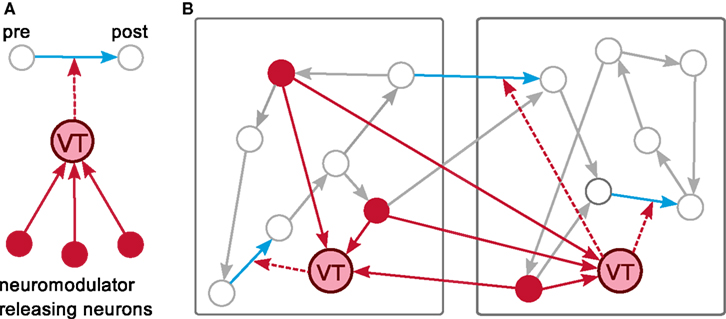
Figure 4. A distributed volume transmitter object. (A) The volume transmitter (VT) collects all spikes from the neurons releasing the neuromodulator into a given volume and delivers them to any associated synapses. (B) An example network is distributed over two machines. The volume transmitter (VT) is duplicated on each machine. It collects globally the spikes of the neuromodulator releasing neurons (red) and delivers them locally to the neuromodulated synapses (blue).

Note that the dynamics of the neuromodulator concentration is calculated by the synapses rather than the volume transmitter. This enables the same framework to be used for a variety of neuromodulatory dynamics as long as they depend only on the spike history. Moreover, the association of a volume transmitter with a specific population of neuromodulator releasing neurons and a specific subset of synapses allows multiple volume transmitters to be defined in the same network model. Thus a network model can represent multiple projection volumes and multiple neuromodulatory interactions.

3.1.2 Managing the spike history

In order to calculate its weight update, a neuromodulated synapse must have access to all the spikes from the neuromodulator releasing neuron population that occurred since the last pre-synaptic spike. This is similar to the requirement of an STDP synapse, which needs access to the post-synaptic spike history since the last pre-synaptic spike (see section 2.1.2). For STDP, this requirement can be met if the post-synaptic neuron stores its spike times (Morrison et al., 2007). To prevent a continual growth in memory requirements as a simulation progresses, the spike times are discarded once all incoming synapses have accessed them. This is an inappropriate strategy for managing the neuromodulatory spikes, as they are typically generated by a population of neurons and so have a substantially higher total rate than the pre-synaptic spike rate. Having a large number of spikes in the history entails proportionally higher computational costs for the algorithm that determines which spikes can be discarded. We propose a novel alternative approach: in addition to delivering a spike history “on demand” when a pre-synaptic spike arrives (Figure 5A), the volume transmitter also delivers its spike history to all associated synapses at regular intervals (Figure 5B). Not only does this combination of an event- and time-driven approach allows us to dispense with an algorithm to discard spikes from the history, it also has the major advantage of enabling the spike history to be stored in a static data structure, rather than a computationally more expensive dynamic data structure.

FIGURE 5

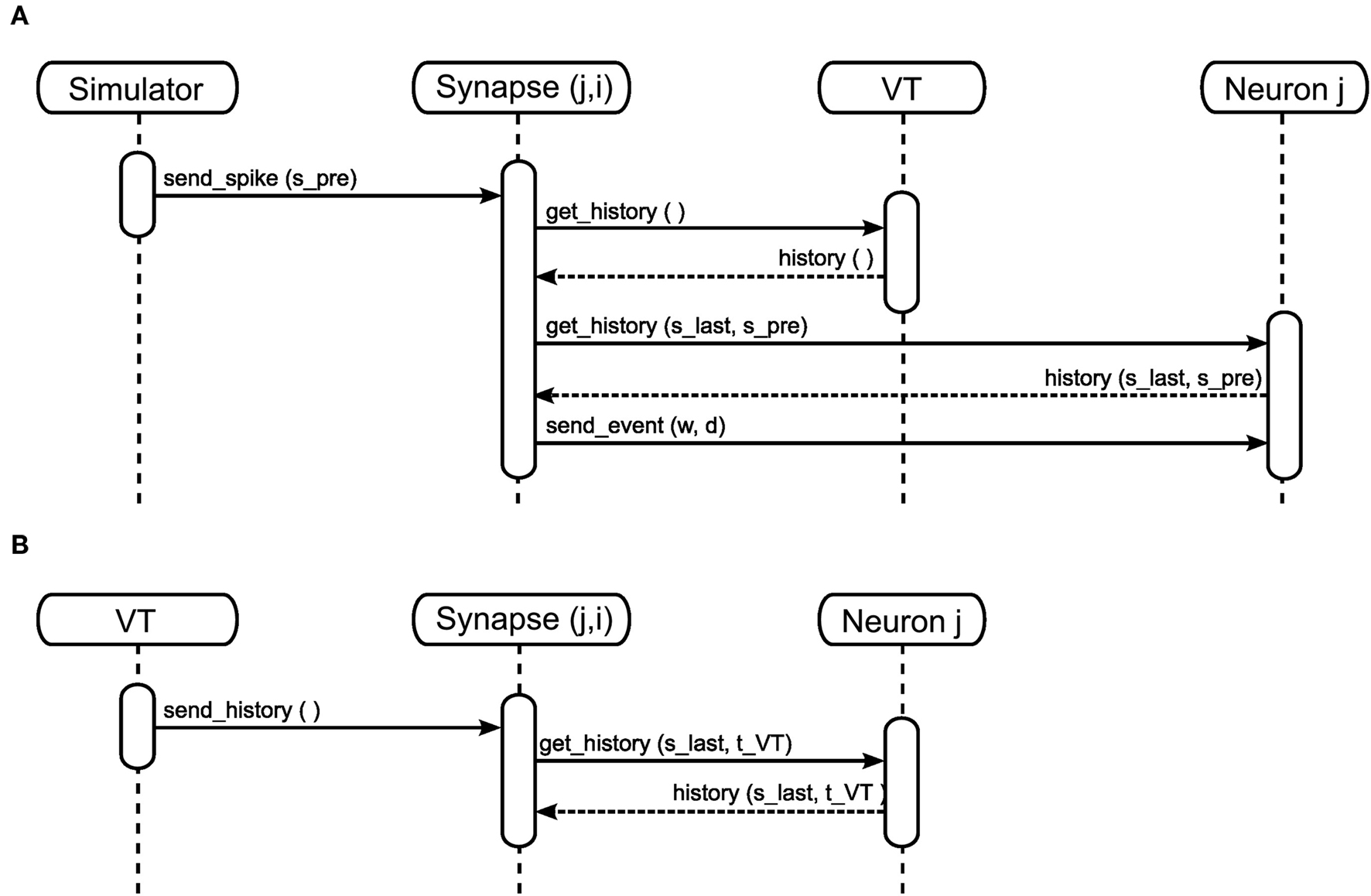
Figure 5. Sequence diagram for neuromodulated synapses in the event-driven (A) and the time-driven (B) mode.

Let us first consider the collection and storing of the spikes of the neuromodulator releasing neurons (Figure 4). A suitable structure to store the spikes is a traditional ring buffer which stores data in a contiguous series of segments as shown in Figure 6, where each segment of the buffer corresponds to one integration time step h (see also Morrison et al., 2005; Morrison and Diesmann, 2006). However, unlike the standard usage of a ring buffer in neuronal network simulations, where only one object reads from it and exactly one read operation from one segment is carried out in each time step, in this situation multiple objects depend on the data and read operations are carried out at unpredictable times and require information from a range of segments at once. Consequently, a new approach to writing to and reading from a ring buffer is necessary, as we describe in the following.

FIGURE 6

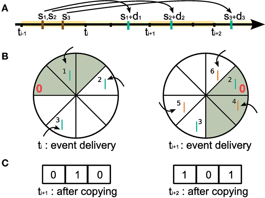
Figure 6. Writing to and reading from the ring buffer of the volume transmitter for event communication in intervals of Δt. In this example, Δt = 3h, where h is the computation time step. (A) Short black bars indicate the grid h imposes on the temporal axis. At time step t_i = iΔt all spikes generated by the neuromodulator releasing neurons in the time interval (t_i−1,t_i] are delivered to the volume transmitter (here: the spike times s₁,s₂,s₃ (brown bars) with propagation delays d₁,d₂,d₃). Blue bars indicate the arrival of the spikes in the projection volume. (B) Ring buffer. Left: at time t_i during event delivery. The neuromodulatory spikes generated in (t_i−1,t_i] (blue bars, labeled by the event id for illustration only) increment the counters at the positions (s_x + d_x − t_i)/h − 1 for x = [1,2,3] from the “front” of the ring buffer (indicated by the red 0). At the end of the event delivery phase, the first Δt/h elements (gray) contain the neuromodulatory spikes due to arrive in the projection volume during (t_i,t_i+1]. Right: at t_i+1 during event delivery. The ’front’ of the buffer has been rotated Δt/h segments clockwise with respect to the buffer at time t_i. Neuromodulatory spikes generated in the time interval (t_i,t_i+1] by the neuromodulator releasing neurons (generation times not shown) are written to the buffer (orange bars), the first Δt/h elements (gray) contain the neuromodulatory spikes due to arrive in the projection volume during (t_i+1,t_i+2]. (C) The spike history buffer. Left: at t_i+1 before the event delivery phase the contents of the top Δt/h elements of the ring buffer at t_i (gray) are copied to the spike history buffer and the counters are reset. Right: at t_i+2 before the event delivery phase the contents of the top Δt/h elements of the ring buffer at t_i+1 are copied to the spike history buffer and the counters are reset.

When a neuromodulator releasing neuron n emits a spike at time s_n, a certain propagation delay d_n is required for the spike to arrive at the projection volume, as illustrated in Figure 6A. Following the description in section 2.1.2, events are communicated after each communication interval of length Δt. Assuming s_n is in the interval (t_i−1,t_i] where t_i = iΔt, the neuromodulatory spike event is communicated between machines at time t_i along with all the other spike events generated in that interval (see Morrison and Diesmann, 2006 for an in depth discussion of the interval borders). Neuromodulatory spike events generated in that interval are delivered to the volume transmitter and sorted into the ring buffer according to their propagation delays. Assigning the “front” of the ring buffer the index 0, for a spike emitted at s_n with a delay d_n, the counter at position (s_n + d_n − t_i)/h − 1 is incremented. This is depicted in the left side of Figure 6B. Setting the ring buffer size to d_max/h, where d_max is the maximal propagation delay, allows the correct order of spikes to be maintained for all possible configurations of spike generation time, communication time, and propagation delay. The communication interval Δt can be set to any integer multiple of h up to d_min, the minimum synaptic propagation delay. A communication interval of Δt = h, where events are communicated in every time step, is the most obvious, naive approach and is probably implemented in at least the first version of almost all simulators. As mentioned in section 2.1.2, a choice of Δt = d_min is the largest possible communication interval that still maintains the correct ordering of events. Maximizing Δt has two advantages: it reduces the communication overhead (see Morrison et al., 2005), and each neuron can perform d_min/h integration time steps as an uninterrupted sequence, improving the cache efficacy considerably (Plesser et al., 2007).

As a result of the sorting, right before the event delivery phase at time t_i+1, the counters for positions in the range [0,Δt/h − 1] give the total number of neuromodulatory spikes that are due to arrive at the synapses in each time step from t_i + h to t_i+1. Counters at positions greater than Δt/h do not necessarily contain the total number of spikes for their respective time steps, as these positions could still receive events at later event delivery phases. At this point, the volume transmitter copies the contents of the ring buffer in the range [0,Δt/h − 1] to a separate spike history buffer of length Δt/h, see Figure 6C. It then resets those counters to zero and rotates the ’front’ of the ring buffer by Δt/h segments as shown in the right side of Figure 6B. Thus the spike history buffer contains all the neuromodulatory spikes that are due to arrive in the projected volume in the interval (t_i,t_i+1], and the ring buffer is prepared to receive the events communicated at time t_i+1.

We now turn to the delivery of the neuromodulatory spikes to the synapses. Let us assume that a synapse associated with a given volume transmitter has received and processed all the neuromodulatory spikes with arrival times up to and including t_i. Therefore the last update time of the synapse s_last is equal to the last neuromodulatory spike time ≤t_i. At time t_i+1 the machines exchange all events generated in the interval (t_i,t_i+1]. If the synapse’s pre-synaptic neuron emits a spike at time s_pre within this interval, all neuromodulatory spikes with t_i < (s_n + d_n) < s_pre still need to be taken into account to calculate the weight dynamics of the synapse up to s_pre. Conversely, neuromodulatory spikes that have already been generated and communicated between machines, but are due to arrive at the projection volume after s_pre, i.e., (s_n + d_n) ≥ s_pre, should not be taken into account. When the synapse is activated during the event delivery phase at t_i+1, it therefore requests the spike history buffer from the volume transmitter, which contains those neuromodulatory spikes for which (s_n + d_n) is in the range (t_i,t_i+1], as described above. Depending on its dynamics, it may also need additional information from the post-synaptic neuron; this is illustrated for the case of dopamine-modulated STDP (Izhikevich, 2007) in Figure 5A, where the post-synaptic spikes between s_last and s_pre must also be requested. At the end of its weight update, the synapse emits an event of the appropriate weight and delay to its post-synaptic target, and sets its variable s_last to the value of s_pre.

Directly after the event delivery phase at t_i+1, the volume transmitter sends its spike history buffer to every associated synapse (see Figure 5B: send_history()). This triggers a weight update for every synapse in which the synapse’s last update time s_last is earlier than the latest spike in the spike history buffer, s_VT. In the dopamine-modulated STDP synapse shown in Figure 5B, calculating the weight update involves requesting all post-synaptic spikes between s_last and s_VT. After calculating the weight update, the synapse sets its variable s_last to the value of s_VT. Thus at the event delivery phase at time t_i+2, each synapse associated with the volume transmitter has received and processed all neuromodulatory spikes with arrival times up to and including t_i+1.

In the above we have described how the synapse can be informed of the spikes necessary for calculating its weight updates without requiring dynamic memory structures or an algorithm to discard spikes that are no longer necessary. The key insight is that event-driven requests for the volume transmitter’s spike history triggered by the arrival of pre-synaptic spikes can be complemented by delivering the spike history at regular intervals in a time-driven fashion. This combined approach does not entail any additional computational costs for the synapse. It must process every neuromodulatory spike, so it makes no difference when the processing takes place, as long as all the information required to calculate a weight update is available when an event is generated. On a global level there are additional costs, as accessing every synapse every Δt interval involves more operations than accessing synapses only on the arrival of pre-synaptic spikes. However, these additional costs can be reduced by transferring the neuromodulatory spikes not in intervals of Δt, but in intervals of n·Δt, where n is an integer. We leave n as a parameter that can be chosen by the user; the consequences of the choice of transfer interval are discussed in section 3.2.3. The only alterations that need to be made to the above description to accommodate this improvement is that the spike history buffer must be correspondingly longer (i.e., n·Δt/h), and spikes must be copied from the ring buffer to the correct section of it.

3.1.3 Establishing a neuromodulated connection

The interaction between the volume transmitter and the synapses requires a bidirectional link. This link from synapse to volume transmitter can be realized by passing the volume transmitter as a parameter when a neuromodulated synapse is defined. The synapse stores a pointer to the volume transmitter and passes its own pointer to the volume transmitter, which maintains a list of associated synapse pointers. For the simulation tool NEST (Gewaltig and Diesmann, 2007) this can be expressed as follows:

1 neuron1=nest.Create("iaf_neuron")
2 neuron2=nest.Create("iaf_neuron")
3 vt=nest.Create("volume_transmitter")
4 nest.SetDefaults("neuromodulated_
    synapse",{"vt": vt[0]})
5 nest.Connect(neuron1, neuron2,
    model="neuromodulated_synapse")

Here we are using NEST’s interface to the Python² programming language PyNEST (Eppler et al., 2009). The population of neurons releasing the neuromodulator are connected to the volume transmitter with standard synaptic connections specifying the propagation delays. For example, in NEST:

6 nest.ConvergentConnect(neuromodulator_neurons,
   vt, delay=d, model="static_synapse")

These operations can be performed in either order.

3.2 Performance

To investigate the efficiency and scalability of our framework, we simulated networks of 10⁴ and 10⁵ neurons incorporating STDP with and without neuromodulation at their excitatory–excitatory synapses as a function of the number of processors used (see section 2.2). The results are illustrated in Figure 7. Figure 7A shows the simulation times for one biological second of the 10⁴ neuron network and Figure 7B shows the corresponding speed-up curves, i.e., how much faster a simulation runs with m machines than with 1 machine (Wilkinson and Allen, 2004). When neuromodulatory spikes are transferred in intervals of Δt = d_min, a supralinear scaling can be observed up to 32 machines, beyond which the scaling is approximately linear. Simulation times are on average 17 times slower than those for the corresponding network incorporating unmodulated STDP. If neuromodulatory spikes are transmitted less often, in intervals of 70·d_min, the reduced number of operations results in a supralinear scaling up to 184 machines. As the number of machines grows, the disparity in simulation times between the neuromodulated and unmodulated networks decreases. The supralinear scaling in all simulations of the 10⁴ neuron network is due to cache effects.

FIGURE 7

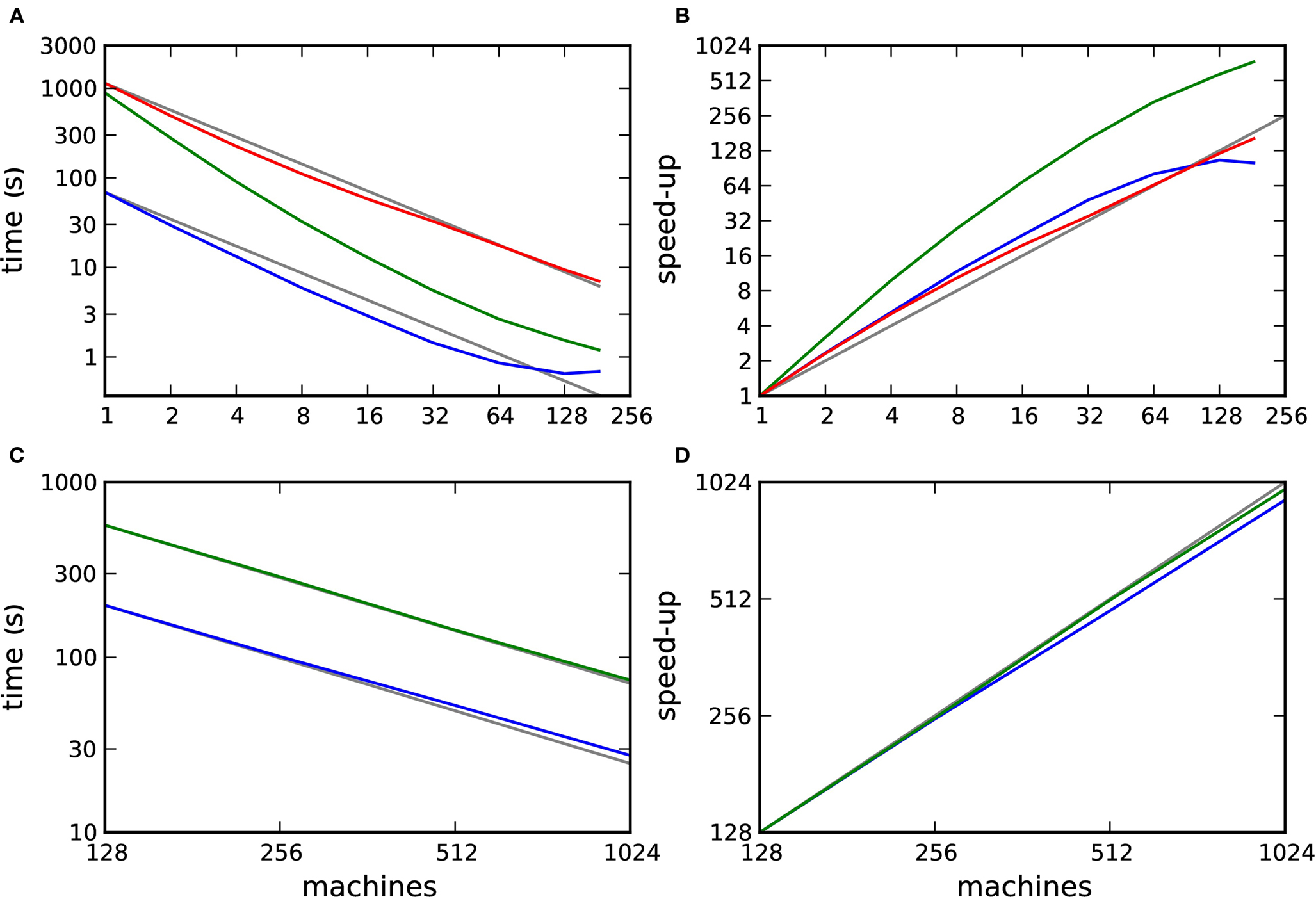
Figure 7. Performance of simulations of networks incorporating STDP with and without neuromodulation. (A) Time to simulate 1 biological second of the 10⁴ neuron network as a function of the number of machines in double logarithmic representation. Neuromodulated STDP with transference of neuromodulatory spikes from the volume transmitter in intervals of d_min (red), 70·d_min (green), unmodulated STDP (blue). (B) Speed-up factor for the simulation times shown in (A). (C) Time to simulate 1 biological second of the 10⁵ neuron network as a function of the number of machines in double logarithmic representation. Neuromodulated STDP with transference of neuromodulatory spikes from the volume transmitter in intervals of 100·d_min (green), unmodulated STDP (blue). (D) Speed-up factor for the simulation times shown in (C). Gray lines indicate linear predictions.

Figures 7C and D show the simulation times for one biological second of the 10⁵ neuron network and the corresponding speed-up curves. The neuromodulated network (transfer interval: 100·d_min) and the unmodulated control network both scale approximately linearly up to 1024 machines. On average the neuromodulated network is 3.2 times slower than the unmodulated network.

These results demonstrate that the framework scales well, up to at least 184 or 1024 machines, depending on the network size. However, they also raise a number of questions. Firstly, in Figures 7A and B we observe that the unmodulated network shows a supralinear scaling up to 64 processors, but then the simulation time saturates at 0.65 s. This suggests that an increase in communication overhead is masking the decrease in computation time. How do the scaling properties of the neuromodulated and unmodulated networks compare if the communication overhead is factored out? Secondly, the neuromodulated network simulations take longer than the unmodulated network simulations. Is this due to the overhead of the volume transmitter infrastructure or due to the increased complexity of the neuromodulated STDP update rule? Finally, faster simulation times are observed when the transfer interval of the volume transmitter is increased. What is the relationship between the performance and the choice of transfer interval? We address these questions in the following three sections.

3.2.1 Saturation due to communication overhead

Let us assume that the simulation time T_sim(m) for m machines is composed of two components: the computing time T_c(m) required to perform the parallel simulation operations such as calculating the neuronal and synaptic dynamics, and the communication time T_ex(m) required to exchange events between machines:

T_sim(m) = T_c(m) + T_ex(m)

The communication time T_ex(m) is a characteristic of the computing architecture used for simulation and typically depends on the number of communicated bytes. As described in section 2.1.2 communication buffers containing spike entries are communicated between machines in time steps of d_min. The number of spikes that each machine sends can be approximated as , where N is the total number of neurons, m the number of machines and λ the average firing rate. If the spikes of successive time steps of length h are separated in the communication buffers by markers, the total number of bytes in each communication buffer is:

where b_spike is the number of bytes to represent the global identifier of a neuron and b_marker is the number of bytes taken up by a marker. In our implementation in NEST, b_spike = b_marker = 8. For a given network simulation we can calculate b(m) and thus the communication time as:

where is the time taken to perform one exchange between m machines of b bytes per machine and T is the biological time simulated. The single exchange time can be determined empirically by measuring the time taken for n calls of the exchange routine for a packet of size b and dividing the total time by n. We measured the single exchange time on our X86 computing cluster by averaging over 1000 function calls exchanging packets of sizes determined by the 10⁴ neuron network simulation (see section 2.2). Figure 8A shows the total communication time T_ex as a function of the number of machines for the 10⁴ neuron network simulation. The communication time increases with the number of machines in proportion to m ln(m), which is to be expected for the algorithm underlying the MPI_Allgather() routine from the MPI library³ used in our implementation. Figure 8B shows the communication time as a percentage of the total simulation time T_sim. The proportion of the simulation time taken up by data exchange increases rapidly with the number of machines. This representation underlines the fact that the communication overhead plays a proportionally bigger role for computationally less expensive applications: the proportion of the total time consumed by data exchange increases more quickly for the unmodulated network simulation than for the neuromodulated cases, rising to more than 40% for the unmodulated network at 184 machines and to 25 and 5% for the neuromodulated networks with transfer intervals of 70·d_min and d_min respectively.

FIGURE 8

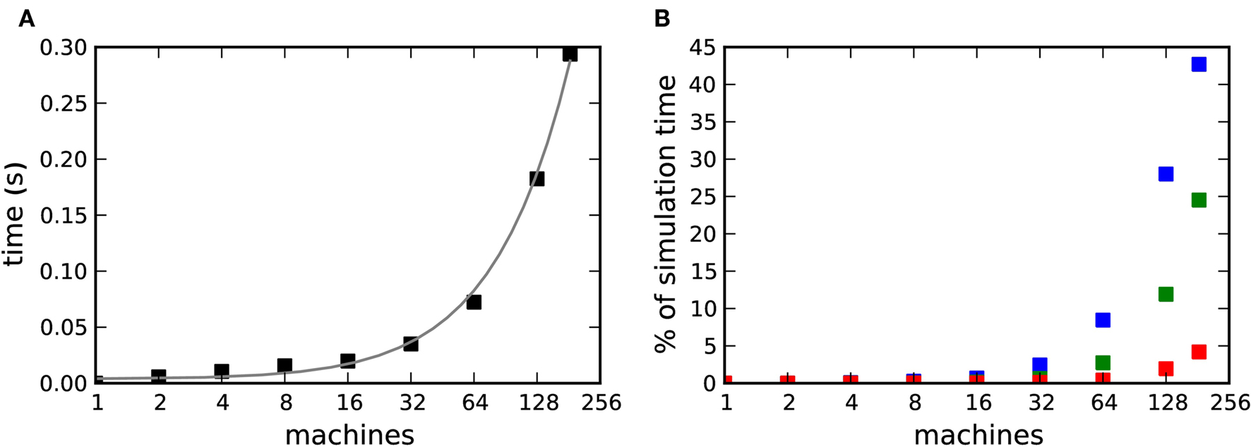
Figure 8. Communication overhead in a distributed simulation of the 10⁴ neuron network. (A) Time required for all necessary data exchanges for a simulation of one biological second as a function of the number of machines. The gray curve is a fit of m·ln(m) to the data. (B) Communication time as a percentage of the total simulation time as a function of the number of machines. Neuromodulated STDP with transference of neuromodulatory spikes from the volume transmitter in intervals of d_min (red), 70·d_min (green), unmodulated STDP (blue).

To obtain the pure computation time T_c(m), we substract the communication time T_ex(m) from the total run time T_sim(m). The result is shown in Figure 9A and the corresponding speed-up curves in Figure 9B.

FIGURE 9

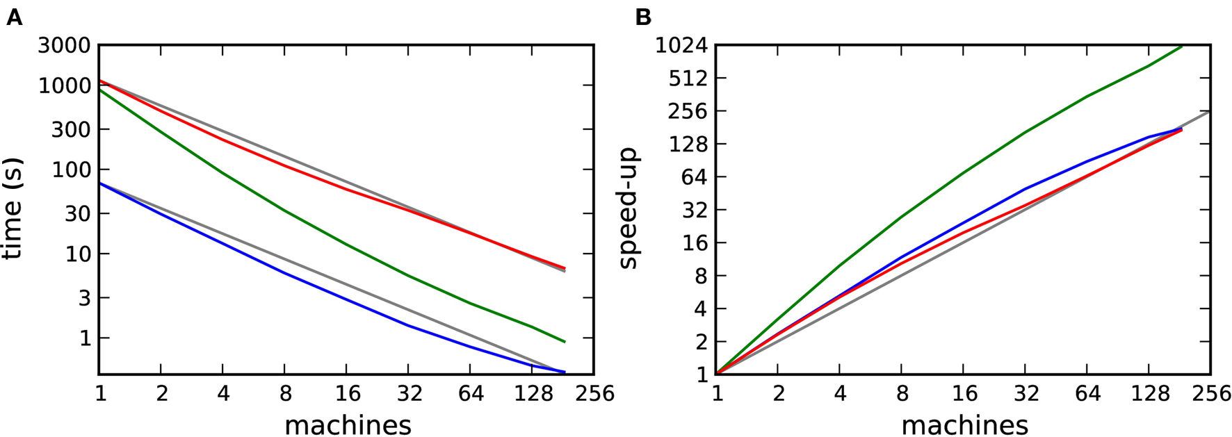
Figure 9. Computation time for a distributed simulation of one biological second of the 10⁴ neuron network. (A) Computation time as a function of number of machines in double logarithmic representation. Neuromodulated STDP with transference of neuromodulatory spikes from the volume transmitter in intervals of d_min (red), 70·d_min (green), unmodulated STDP (blue). (B) Speed-up factor for the simulation times shown in (A). Gray lines indicate linear predictions.

The effect on the scaling of the neuromodulated network simulations is small. However, the saturation of simulation time for the unmodulated network observed in Figures 7A and B is no longer visible, demonstrating that the saturation was due to communication overhead rather than suboptimal simulation algorithms. All network simulations exhibit linear scaling or better up to 184 machines.

3.2.2 Dependence of performance on the neuromodulatory firing rate

Figures 7 and 9 show that the simulation times for the neuromodulated network simulations are much longer than for the unmodulated network simulations. This could be due to the computational cost of the volume transmitter overhead, or to the increased complexity of the neuromodulated STDP update rule, which depends not only on the pre- and post-synaptic rate but also on the rate of the population of neuromodulator releasing neurons (see section 2.2). For the curves shown in Figures 7 and 9, the size of the neuromodulator releasing population N_nm was set to 50, resulting in a neuromodulatory firing rate of ≈500 Hz.

Figure 10 shows the dependence of the simulation time for the 10⁴ neuron network on 184 processors as a function of the firing rate of the neuromodulatory population. The different firing rates are realized by varying the number of neuromodulator releasing neuron N_nm from 0 to 60 in steps of 5. Note that the network activity is not affected by the choice of N_nm on the time scale of one second, so the pre- and post-synaptic firing rates are constant for all values of N_nm. A linear increase of simulation time with neuromodulatory firing rate can be observed, with a greater slope for a transfer interval of d_min than for 70·d_min. For a neuromodulatory spike rate of 0 Hz, the simulation times for the neuromodulated networks are only slightly larger than for the unmodulated network. These results demonstrate that the large disparity in simulation times observed between the neuromodulated and unmodulated simulations is not due to overheads related to the volume transmitter infrastructure but to the increased computational complexity of the neuromodulated STDP update rule. As a further test, we carried out an experiment for a neuromodulatory firing rate of 500 Hz in which the volume transmitter infrastructure transfers the neuromodulatory spikes to the synapse, but the synapse performs the unmodulated STDP update rule, i.e., the synapse ignores the transferred spikes. In this case the simulation times are reduced to those of the unmodulated STDP control case (data not shown).

FIGURE 10

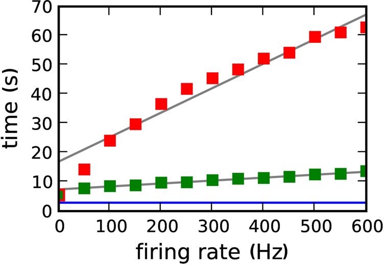
Figure 10. Simulation time for one biological second of the 10⁴ neuron network for 184 machines as a function of the neuromodulatory firing rate. Neuromodulated STDP with transference of neuromodulatory spikes from the volume transmitter in intervals of d_min (red squares), 70·d_min (green squares). The blue line indicates the simulation time for the unmodulated network; the gray lines are linear fits to the data.

These results confirm the decision to store the neuromodulatory spikes in a fixed-size buffer and ensure all spikes are taken into consideration by regular updates of the associated synapses. The alternative approach, to store spikes in a dynamically sized buffer and update synapses only on demand, requires the use of an algorithm to discard spikes that have already been processed. The complexity of such an algorithm is linear in the number of spikes in the buffer, therefore such a scheme would entail proportionally higher costs with increased neuromodulatory spike rate, whereas the cost for our framework is approximately constant.

3.2.3 Dependence of performance on the transfer interval

Figures 7 and 10 show that faster simulation times are achieved with a transfer time of 70·d_min than with a transfer time of d_min for all numbers of machines and all neuromodulatory rates. This is unsurprising, as the longer transfer time entails proportionally fewer transfer operations: the number of transfer operations is given by T/(n·d_min), where T is the biological time simulated. However, a longer transfer time also requires a larger data structure to hold all the buffered spikes. As increasing the memory used by an application will generally decrease its speed, optimizing performance may require a trade-off to be found between reducing the number of operations and limiting the memory requirements.

To obtain the dependence of the simulation time on the transfer time, we carried out simulations of the 10⁴ neuron network whilst varying the parameter n, where n·d_min is the transfer interval for communicating spikes in a time-driven fashion from the volume transmitter to the synapses (see section 3.1.2). The results are shown in Figure 11A. By plotting the simulation time as a function of 1/n in Figure 11B, we can see that the simulation time is indeed proportional to 1/n for n>2. For smaller values of n the neuromodulator spike buffers are sometimes empty, in which case the transfer operation is omitted, leading to a faster simulation time than the linear prediction. These results demonstrate that increasing the memory requirements of the volume transmitter does not result in a decrease in performance, so in practice a large value of n should be selected.

FIGURE 11

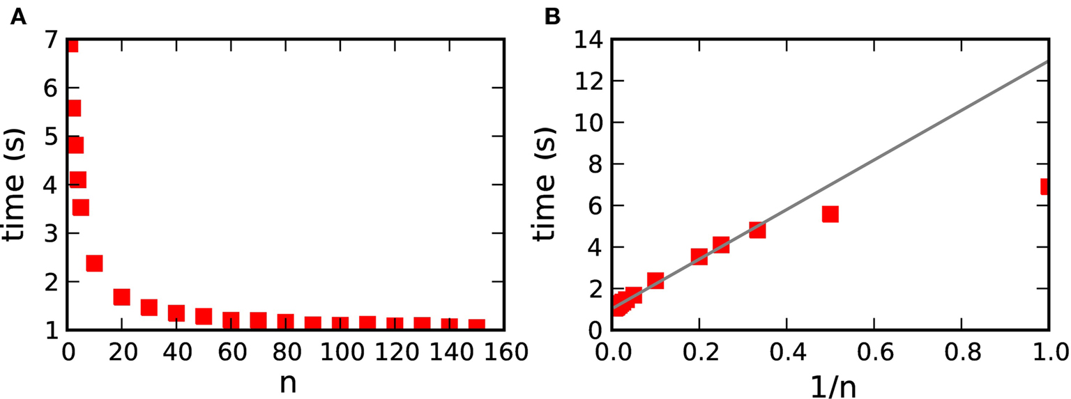
Figure 11. Simulation time for one biological second of the 10⁴ neuron network for 184 machines with respect to n, where n·d_min is the transfer interval of the volume transmitter. (A) Simulation time as a function of n. (B) Simulation time as a function of 1/n. The gray line shows the linear fit for n>2.

Discussion

Neuromodulated plasticity has recently become a hot topic in computational as well as experimental neuroscience. There is evidence for neuromodulator involvement in many cognitive functions, such as attention or reward learning (Reynolds et al., 2001; Hasselmo and McGaughy, 2004). On the cellular level it has been shown that long-range neuromodulatory systems strongly influence the induction of spike-timing dependent plasticity (see Pawlak et al., 2010 in this special issue). Neuromodulated plasticity is a strong candidate for a mechanism that links synaptic plasticity to system level learning (Seung, 2003; Xie and Seung, 2004; Baras and Meir, 2007; Florian, 2007; Izhikevich, 2007; Legenstein et al., 2008; Potjans et al., 2009b, 2010Vasilaki et al., 2009; Pawlak et al., 2010, this special issue). However, so far in most spiking neural networks models implementing neuromodulated synaptic plasticity, the signal is injected externally into the network rather than being generated by the network itself (but see Izhikevich, 2007 and Legenstein et al., 2008). Furthermore, technical details about the implementation of neuromodulated plasticity in spiking neural networks have not been provided. Due to this lack models cannot be easily reproduced or extended by the wider modeling community.

Here, we present for the first time a general framework for the efficient implementation of neuromodulated plasticity in time-driven distributed simulations where the neuromodulatory signal is generated within the network. The presented framework paves the way for the investigation of a wide range of neural circuits which generate and exploit a neuromodulatory signal to carry out cognitive functions, such as dopamine-driven learning and noradrenaline-mediated stress response. The framework is general in the sense that it does not rely on a particular implementation language, neuromodulator, or neuromodulated plasticity and makes few and easily fulfilled assumptions about the data structures and algorithms of the underlying simulation tool. The main difficulty in the implementation of neuromodulated plasticity in distributed simulations is how to inform the neuromodulated synapses efficiently about the non-local neuromodulatory signal, which is typically generated by a population of neurons on different machines than either the pre- or the post-synaptic neuron. We solved this problem by introducing a new object called “volume transmitter,” which represents the neuromodulatory signal available in a certain volume by globally collecting all the spikes from neurons in a specified neuromodulator releasing population and transferring the spikes to a user-specified subset of local synapses. We propose a hybrid algorithm for the transfer of spikes from the volume transmitter to the neuromodulated synapses. In addition to the delivery triggered by every pre-synaptic spike, the neuromodulatory spike history is delivered in discrete time intervals of n·Δt, where n is an integer and Δt the communication interval of the network. This has three advantages over a purely event-based transfer: first, the neuromodulatory spikes can be stored in a static data structure; second, no additional algorithm is required to determine which spikes can be cleared from the history; and third, the memory requirements are known and fixed regardless of the network activity. The technology is fully implemented and available in NEST including an example and can be controlled through the application interface to the Python programming language (Eppler et al., 2009).

Our results show that simulation time is proportional to 1/n for n>2; this is due to the decrease in the number of operations performed. As no deterioration in performance can be observed for large n as a result of the larger memory structure, in practice a large n should be selected. For a suitably large choice of n, our framework exhibits supralinear scaling up to 184 machines on simulations of a balanced random network of 10⁴ neurons incorporating neuromodulated STDP in its excitatory to excitatory connections. Further, linear scaling can be observed up to 1024 machines on simulations of a network containing 10⁵ neurons with a biologically realistic number of inputs to each neuron (10⁴) and connectivity (10%), corresponding to 1 mm³ of mammalian cortex. The scaling properties of the neuromodulated network simulations are comparable to, or better than, that of an unmodulated network simulation. Additionally, our framework does not incur any additional costs with increased firing rate of the neuromodulatory neuron population other than those necessarily imposed by the complexity of the neuromodulated synaptic update rules. Although our motivation was to provide a framework capable of meeting the demands of very large distributed neuronal network simulations, it can be used without adaptation for the serial simulation of smaller-scale networks in which the neuromodulatory signal is generated within the network.

In the context of analyzing the benchmark simulations we developed a technique to determine what proportion of the run time of a simulation is taken up by communication between machines. This generally applicable technique enables a developer of distributed software to distinguish a saturation due to communication overheads from one due to a suboptimally implemented algorithm.

Although our hybrid communication strategy was developed in the context of the particular challenges of neuromodulated plasticity, it could well enable a more efficient formulation of algorithms to model unmodulated plasticity such as STDP. Combining event-driven weight updates triggered by pre-synaptic spikes with time-driven updates at regular intervals would permit also the post-synaptic spike history to be stored in a static data structure and remove the need for an algorithm to discard spikes that are no longer relevant. However, as one spike history structure is required for each post-synaptic neuron (rather than one for an entire neuromodulatory population), the memory requirements of the simulation will depend more strongly on the choice of transfer interval. In future work, we will investigate the trade-off between reducing the number of transfer operations and increasing the memory requirements.

We have formulated the neuromodulator dynamics as a dynamics on a graph where the interaction is mediated by point events. This integrates well into the representation of spiking neuronal networks used for large-scale simulation. In addition we have decided to place the dynamics of the neuromodulatory signal at the site of the individual synapse. An alternative approach would be to low-pass filter the neuromodulatory spikes on each machine and then exchange and add the filtered signals between machines. As the global signal is mostly likely to be slow, this exchange could perhaps be performed less often than the communication of spikes in intervals of Δt. However, this alternative approach has several disadvantages with respect to our proposal. First, whereas the alternative proposal would require additional communication to exchange the filtered signals among machines, our framework causes no additional communication costs, as spikes have to be exchanged anyway in the distributed framework. Therefore, an approximate solution is unlikely to be more efficient. Second, our approach has the advantage that neuromodulated synaptic dynamics where changes of the synaptic state depend on the instantaneous value of the neuromodulator level can be implemented exactly. Therefore, even in the case that an approximate solution is more efficient for a particular application, it would be useful to have the exact implementation at hand for a verification of the results. Third, in our proposal the same framework can be used for a variety of different neuromodulators with different neuromodulatory dynamics, assuming the neuromodulator level can be calculated solely on the basis of the spike train of the releasing population. However, this generality comes at a price. The time course of a neuromodulator, which is probably essentially identical within a certain volume of cortex, is recomputed in every synapse, resulting in redundant operations. Moreover, we assumed that each spike of the neuromodulator releasing population contributes the same amount to the neuromodulator concentration. If necessary, these disadvantages can be remedied in the context of a specific scientific question by developing more specialized versions of the volume transmitter that calculate the dynamics of the neuromodulator under investigation and then deliver the results of this calculation to the synapses.

Our solution is based on the assumption that it is sufficiently accurate to represent the times of the neuromodulatory spikes on the grid defined by the computation step size. The framework can be modified to process “off-grid” spike times, but at the cost of maintaining dynamic data structures in the volume transmitter which would result in a deterioration of performance. A further limitation of our framework is that it has no capacity to represent spatial variations in neuromodulator concentration within the population of synapses such as diffusion processes. Recently, a simulation tool has been presented which considers diffusion processes by explicitly modeling the extracellular space (Zubler and Douglas, 2009).

As our solution enables networks to be simulated that generate their own modulatory signals, it paves the way for the investigation of closed-loop functional models. We already successfully applied our framework to a model that implements temporal-difference learning based on dopamine modulated plasticity to solve a navigation problem (Potjans et al., 2009c). Even though the network investigated here was comparatively small (order of 10³ neurons), systematic investigation of it required distributed computing; although the plasticity process occurs on a time scale of tens of milliseconds, the learning process on the network level takes place on a time scale of minutes to hours. The user has full flexibility to assign the volume transmitter to specific groups of neuromodulator releasing neurons and neuromodulated synapses, thus allowing the simulation of multiple volumes with different neuromodulator concentrations or multiple neuromodulators with different dynamics in the same network. Our results suggest that the framework will scale up to much larger networks than those investigated here. This will enable the investigation of “brain-scale” networks modeling circuits made up of several brain areas. One possible application is to investigate the role of neuromodulators such as acetylcholine in the cortex simultaneously with its generation process, which takes place in subcortical areas. It is our hope that our novel technology will make it easy for computational neuroscientists to study sophisticated models with interesting system-level behavior based on neuromodulated plasticity.

Conflict of Interest Statement

The authors declare that the research was conducted in the absence of any commercial or financial relationships that could be construed as a potential conflict of interest.

Acknowledgments

We are most grateful to Hans Ekkehard Plesser for language legality consultation. We also thank the editor and the reviewers for the constructive interaction which helped us to considerably improve the integration of our work into the special issue. Partially funded by DIP F1.2, BMBF Grant 01GQ0420 to the Bernstein Center for Computational Neuroscience Freiburg, EU Grant 15879 (FACETS), the Junior Professor Program of Baden-Württemberg, “The Next-Generation Integrated Simulation of Living Matter” project, part of the Development and Use of the Next-Generation Supercomputer Project of the Ministry of Education, Culture, Sports, Science and Technology (MEXT) of Japan and the Helmholtz Alliance on Systems Biology. Access to supercomputing facility through JUGENE-Grant JINB33.

Footnotes

1. ^http://www.fz-juelich.de/jsc/jugene/
2. ^http://www.python.org
3. ^http://www.open-mpi.org/

References

Agnati, L., Zoli, M., Strömberg, I., and Fuxe, K. (1995). Intercellular communication in the brain: wiring versus volume transmission. Neuroscience 69, 711–726.

Pubmed Abstract | Pubmed Full Text | CrossRef Full Text

Ananthanarayanan, R., and Modha, D. S. (2007). “Anatomy of a cortical simulator,” in Supercomputing 2007: Proceedings of the ACM/IEEE SC2007 Conference on High Performance Networking and Computing (New York, NY: Association for Computing Machinery).

Antonov, I., Antonova, I., Kandel, E. R., and Hawkins, R. D. (2003). Activity-dependent presynaptic facilitation and hebbian LTP are both required and interact during classical conditioning in aplysia. Neuron 37, 135–147.

Pubmed Abstract | Pubmed Full Text | CrossRef Full Text

Arbuthnott, G., and Wickens, J. (2007). Space, time and dopamine. Trends Neuroscience 30, 62–69.

CrossRef Full Text

Baras, D., and Meir, R. (2007). Reinforcement learning, spike-time-dependent plasticity, and the BCM rule. Neural Comput. 19, 2245–2279.

Pubmed Abstract | Pubmed Full Text | CrossRef Full Text

Berridge, C. W., and Waterhouse, B. D. (2003). The locus coeruleus-noradrenergic system: modulation of behavioral state and state-dependent cognitive processes. Brain Res. Brain Res. Rev. 42, 33–84.

Pubmed Abstract | Pubmed Full Text | CrossRef Full Text

Bi, G., and Poo, M. (2001). Synaptic modification by correlated activity: Hebb’s postulate revisited. Annu. Rev. Neurosci. 24, 139–66.

Pubmed Abstract | Pubmed Full Text | CrossRef Full Text

Bi, G.-Q., and Poo, M.-M. (1998). Synaptic modifications in cultured hippocampal neurons: dependence on spike timing, synaptic strength, and postsynaptic cell type. J. Neurosci. 18, 10464–10472.

Pubmed Abstract | Pubmed Full Text

Braitenberg, V., and Schüz, A. (1998). Cortex: Statistics and Geometry of Neuronal Connectivity, 2nd Edn. Berlin: Springer-Verlag.

Brette, R., Rudolph, M., Carnevale, T., Hines, M., Beeman, D., Bower, J. M., Diesmann, M., Morrison, A., Goodman, P. H., Harris, F. C. Jr., Zirpe, M., Natschläger, T., Pecevski, D., Ermentrout, B., Djurfeldt, M., Lansner, A., Rochel, O., Vieville, T., Muller, E., Davison, A. P., El Boustani, S., and Destexhe, A. (2007). Simulation of networks of spiking neurons: a review of tools and strategies. J. Comput. Neurosci. 23, 349–398.

Pubmed Abstract | Pubmed Full Text | CrossRef Full Text

Cooper, J., Bloom, F., and Roth, R. (2002). The Biochemical Basis of Neuropharmacology. New York, Oxford: Oxford University Press.

Deco, G., and Thiele, A. (2009). Attention: oscillations and neuropharmacology. Eur. J. Neurosci. 30, 347–354.

Pubmed Abstract | Pubmed Full Text | CrossRef Full Text

Eppler, J. M., Helias, M., Muller, E., Diesmann, M., and Gewaltig, M. (2009). PyNEST: a convenient interface to the NEST simulator. Front. Neuroinformatics 2, 12.

Florian, R. V. (2007). Reinforcement learning through modulation of spike-timing-dependent synaptic plasticity. Neural Comput. 19, 1468–1502.

Pubmed Abstract | Pubmed Full Text | CrossRef Full Text

Garris, P. A., Ciolkowski, E. L., Pastore, P., and Wightman, R. M. (1994). Efflux of dopamine from the synaptic cleft in the nucleus accumbens of the rat brain. J. Neurosci. 14, 6084–6093.

Pubmed Abstract | Pubmed Full Text

Gerstner, W., Kempter, R., van Hemmen, J. L., and Wagner, H. (1996). A neuronal learning rule for sub-millisecond temporal coding. Nature 383, 76–78.

Pubmed Abstract | Pubmed Full Text | CrossRef Full Text

Gewaltig, M.-O., and Diesmann, M. (2007). NEST (Neural Simulation Tool). Scholarpedia J. 2, 1430.

CrossRef Full Text

Hammarlund, P., and Ekeberg, O. (1998). Large neural network simulations on multiple hardware platforms. J. Comput. Neurosci. 5, 443–459.

Pubmed Abstract | Pubmed Full Text | CrossRef Full Text

Hanuschkin, A., Kunkel, S., Helias, M., Morrison, A., and Diesmann, M. (2010). A general and efficient method for incorporating precise spike times in globally time-driven simulations. Front. Neuroinform. 4:133. doi: 10.3389/fninf.2010.00113.

CrossRef Full Text

Harris, J., Baurick, J., Frye, J., King, J., Ballew, M., Goodman, P., and Drewes, R. (2003). A novel parallel hardware and software solution for a large-scale biologically realistic cortical simulation. Technical Report, University of Nevada, Reno, NV.

Hasselmo, M., and McGaughy, J. (2004). High acetylcholine levels set circuit dynamics for attention and encoding and low acetylcholine levels set dynamics for consolidation. Prog. Brain Res. 145, 207–231.

Pubmed Abstract | Pubmed Full Text | CrossRef Full Text

Hebb, D. O. (1949). The Organization of Behavior: A Neuropsychological Theory. New York: John Wiley and Sons.

Herrero, J. L., Roberts, M. J., Delicato, L. S., Gieselmann, M. A., Dayan, P., and Thiele, A. (2008). Acetylcholine contributes through muscarinic receptors to attentional modulation in v1. Nature 454, 1110–1113.

Pubmed Abstract | Pubmed Full Text | CrossRef Full Text

Izhikevich, E. M. (2007). Solving the distal reward problem through linkage of STDP and dopamine signaling. Cereb. Cortex 17, 2443–2452.

Pubmed Abstract | Pubmed Full Text | CrossRef Full Text

Lamport, L. (1978). Time, clocks, and the ordering of events in a distributed system. Commun. ACM 21, 558–565.

CrossRef Full Text

Legenstein, R., Pecevski, D., and Maass, W. (2008). A learning theory for reward-modulated spike-timing-dependent plasticity with application to biofeedback. PLoS Comput. Biol. 4, e1000180. doi: 10.1371/journal.pcbi.1000180.

Pubmed Abstract | Pubmed Full Text | CrossRef Full Text

Markram, H., Lübke, J., Frotscher, M., and Sakmann, B. (1997). Regulation of synaptic efficacy by coincidence of postsynaptic APs and EPSPs. Science 275, 213–215.

Pubmed Abstract | Pubmed Full Text | CrossRef Full Text

Markram, H., and Tsodyks, M. (1996). Redistribution of synaptic efficacy between neocortical pyramidal neurons. Nature 382, 807–810.

Pubmed Abstract | Pubmed Full Text | CrossRef Full Text

Montague, P. R., McClure, S. M., Baldwin, P., Phillips, P. E., Budygin, E. A., Stuber, G. D., Kilpatrick, M. R., and Wightman, R. M. (2004). Dynamic gain control of dopamine delivery in freely moving animals. J. Neurosci. 24, 1754–1759.

Pubmed Abstract | Pubmed Full Text | CrossRef Full Text

Moreau, A., Amar, M., Le Roux, N., Morel, N., and Fossier, P. (2010). Serotoninergic fine-tuning of the excitation–inhibition balance in rat visual cortical networks. Cereb. Cortex 20, 456–467.

Pubmed Abstract | Pubmed Full Text | CrossRef Full Text

Morrison, A., Aertsen, A., and Diesmann, M. (2007). Spike-timing dependent plasticity in balanced random networks. Neural Comput. 19, 1437–1467.

Pubmed Abstract | Pubmed Full Text | CrossRef Full Text

Morrison, A., and Diesmann, M. (2006). “Maintaining causality in discrete time neuronal network simulations,” in Proceedings of the Potsdam Supercomputer School 2005, Germany.

Morrison, A., and Diesmann, M. (2008). “Maintaining causality in discrete time neuronal network simulations,” in Lectures in Supercomputational Neuroscience: Dynamics in Complex Brain Networks, Understanding Complex Systems, eds P. Beim Graben, C. Zhou, M. Thiel, and J. Kurths (Springer, Verlag: Berlin Heidelberg), 267–278.

Morrison, A., Diesmann, M., and Gerstner, W. (2008). Phenomenological models of synaptic plasticity based on spike-timing. Biol. Cybern. 98, 459–478.

Pubmed Abstract | Pubmed Full Text | CrossRef Full Text

Morrison, A., Mehring, C., Geisel, T., Aertsen, A., and Diesmann, M. (2005). Advancing the boundaries of high connectivity network simulation with distributed computing. Neural Comput. 17, 1776–1801.

Pubmed Abstract | Pubmed Full Text | CrossRef Full Text

Morrison, A., Straube, S., Plesser, H. E., and Diesmann, M. (2007). Exact subthreshold integration with continuous spike times in discrete time neural network simulations. Neural Comput. 19, 47–79.

Pubmed Abstract | Pubmed Full Text | CrossRef Full Text

Nordlie, E., Gewaltig, M.-O., and Plesser, H. E. (2009). Towards reproducible descriptions of neuronal network models. PLoS Comput. Biol. 5, e1000456.doi: 10.1371/journal.pcbi.1000456.

Pubmed Abstract | Pubmed Full Text | CrossRef Full Text

Pawlak, V., Wickens, J. R., Kirkwood, A., and Kerr, J. N. D. (2010). Timing is not everything: neuromodulation opens the STDP gate. Front. Syn. Neurosci. 2:146. doi: 10.3389/fnsyn.2010.00146.

CrossRef Full Text

Pecevski, D., Natschläger, T., and Schuch, K. (2009). PCSIM: a parallel simulation environment for neural circuits fully integrated with python. Front. Neuroinformatics 3:11. doi: 10.3389/neuro.11.011.2009.

Pubmed Abstract | Pubmed Full Text | CrossRef Full Text

Plesser, H. E., Eppler, J. M., Morrison, A., Diesmann, M., and Gewaltig, M.-O. (2007). “Efficient parallel simulation of large-scale neuronal networks on clusters of multiprocessor computers,” in Euro-Par 2007: Parallel Processing, volume 4641 of Lecture Notes in Computer Science, eds A.-M. Kermarrec, L. Bougé, and T. Priol (Berlin: Springer-Verlag), 672–681.

Potjans, W., Morrison, A., and Diesmann, M. (2009a). Implementing neuromodulated plasticity in distributed simulations. Front. Neuroinformatics Conference Abstract: 2nd INCF Congress of Neuroinformatics. doi: 10.3389/conf.neuro.11.2009.08.043.

CrossRef Full Text

Potjans, W., Morrison, A., and Diesmann, M. (2009b). A spiking neural network model of an actor-critic learning agent. Neural Comput. 21, 301–339.

CrossRef Full Text

Potjans, W., Morrison, A., and Diesmann, M. (2009c). A spiking temporal-difference learning model based on dopamine-modulated plasticity. BMC Neurosci. 10(Supp 1), 140.

CrossRef Full Text

Reynolds, J. N. J., Hyland, B. I., and Wickens, J. R. (2001). A cellular mechanism of reward-related learning. Nature 413, 67–70.

Pubmed Abstract | Pubmed Full Text | CrossRef Full Text

Schultz, W., Dayan, P., and Montague, P. R. (1997). A neural substrate of prediction and reward. Science 275, 1593–1599.

Pubmed Abstract | Pubmed Full Text | CrossRef Full Text

Seung, H. S. (2003). Learning spiking neural networks by reinforcement of stochastic synaptic transmission. Neuron 40, 1063–1073.

Pubmed Abstract | Pubmed Full Text | CrossRef Full Text

Song, S., and Abbott, L. F. (2001). Cortical development and remapping through spike timing-dependent plasticity. Neuron 32, 339–350.

Pubmed Abstract | Pubmed Full Text | CrossRef Full Text

Song, S., Miller, K. D., and Abbott, L. F. (2000). Competitive Hebbian learning through spike-timing-dependent synaptic plasticity. Nat. Neurosci. 3, 919–926.

Pubmed Abstract | Pubmed Full Text | CrossRef Full Text

Thomson, A. M., and Deuchars, J. (1994). Temporal and spatial properties of local circuits in neocortex. Trends Neurosci. 17, 119–126.

Pubmed Abstract | Pubmed Full Text | CrossRef Full Text

Vasilaki, E., Frémaux, N., Urbanczik, R., Senn, W., and Gerstner, W. (2009). Spike-based reinforcement learning in continuous state and action space: When policy gradient methods fail. PLoS Comput. Biol. 5, e1000586. doi: 10.1371/journal.pcbi.1000586.

Pubmed Abstract | Pubmed Full Text | CrossRef Full Text

Wilkinson, B., and Allen, M. (2004). Parallel Programming: Techniques and Applications Using Networked Workstations and Parallel Computers (2 ed.). Prentice Hall.

Xie, X., and Seung, H. S. (2004). Learning in neural networks by reinforcement of irregular spiking. Phys. Rev. E 69, 41909.

CrossRef Full Text

Zoli, M., and Agnati, L. F. (1996). Wiring and volume transmission in the central nervous system: The concept of closed and open synapses. Prog. Neurobiol. 49, 363–380.

Pubmed Abstract | Pubmed Full Text

Zoli, M., Jansson, A., Syková, E., Agnati, L. F., and Fuxe, K. (1999). Volume transmission in the cns and its relevance for neuropsychopharmacology. Trends Pharmacol. Sci. 20, 142–150.

Pubmed Abstract | Pubmed Full Text | CrossRef Full Text

Zubler, F., and Douglas, R. (2009). A framework for modeling the growth and development of neurons and networks. Front. Comput. Neurosci. 3:25. doi: 10.3389/neuro.10.025.2009.

Pubmed Abstract | Pubmed Full Text | CrossRef Full Text