Rate dynamics of leaky integrate-and-fire neurons with strong synapses

1 Introduction

Instantaneous firing rates are commonly used to describe either the compound spiking activity of neuron ensembles (population rate) or the trial-averaged response of individual neurons to multiple repetitions of the same stimulus. The dynamics of firing rates is often studied by means of population or firing-rate models. The main purpose of such models is to reduce the dimensionality and complexity of the microscopic dynamics of neural networks in order to obtain tools which allow mathematical treatment, efficient simulation, and intuitive understanding. Since the seminal studies of Wilson and Cowan (1972) and Knight (1972a), a zoo of population models has emerged in the literature. Often, they have to be considered purely phenomenological descriptions. Under simplifying assumptions, they can be mathematically derived from the single-neuron dynamics. In many cases, however, the mathematics of these “reduced” models is still very complex.

A standard solution to this problem is to study the dynamics in a restricted region of the state space. By means of linear-response analysis, for example, one can describe the time-dependent output firing rate r(t) of a population of neurons (or an ensemble of trials) in response to some input signal x(t) in the vicinity of a stationary working point (x₀, r₀) for small perturbations Δx(t) = x(t) –x₀. The outcome of this analysis is the system’s impulse response¹ h₀(t), or, in the frequency domain, the transfer function H₀(f) = 𝕱 [h₀(t)](f)²,³. Once the impulse response h₀(t) is known, one can predict the output rate r(t) for any arbitrary, but sufficiently small, stimulus perturbation Δx(t) by a convolution,⁴

The output rate r₀ in response to a constant input x₀ is typically described by a nonlinear activation function r₀ = g(x₀) (“f-I curve”). Note, that in several studies the activation function is called “transfer function” (e.g., Destexhe and Sejnowski, 2009). Following the terminology of linear-systems theory, we use the term “transfer function” exclusively for the Fourier transform of the impulse response.

The dynamical response properties of neuron populations, i.e., the properties of the transfer function H₀(f), have been extensively studied both theoretically (e.g., Knight, 1972a; Gerstner, 2000; Brunel et al., 2001; Lindner and Schimansky-Geier, 2001; Fourcaud and Brunel, 2002; Mattia and Del Giudice, 2002; Fourcaud-Trocmé et al., 2003; Naundorf et al., 2005; Richardson, 2007; Pressley and Troyer, 2009) and experimentally (Knight, 1972b; Silberberg et al., 2004; Köndgen et al., 2008; Blomquist et al., 2009; Boucsein et al., 2009). One of the major insights has been that populations of neurons can track time-varying input signals much faster than single cells. Theoretical studies have shown that the shape of the transfer function H₀(f) depends crucially on the properties of the single-neuron dynamics (Knight, 1972a; Fourcaud-Trocmé et al., 2003; Naundorf et al., 2005; Richardson, 2007) and on the filter properties of the synapses (Brunel et al., 2001).

Most previous studies have investigated the population rate in response to a time-varying noisy input current injected into the soma of the cells. At each instance in time t, the current amplitudes for the ensemble of neurons (trials) were assumed to be uncorrelated and to follow a normal distribution with mean μ(t) and variance σ²(t). Strictly speaking, this corresponds to a scenario where spikes from presynaptic sources arrive at the target cells independently with infinite rate, and where the impact of each spike on the postsynaptic neuron, i.e., the synaptic weight, is infinitesimal (“diffusion approximation”; Johannesma, 1968). For many neural systems, these assumptions are violated: In the mammalian neocortex, for example, a considerable fraction of excitatory synapses gives rise to postsynaptic potentials (PSPs) which cannot be considered small (PSP amplitudes larger than 1 mV; see, e.g., Fetz et al., 1991; Song et al., 2005; Bannister and Thomson, 2007; Lefort et al., 2009). The same holds for hippocampal neurons (Fetz et al., 1991). In the early visual pathway, synapses between retinal ganglion cells and cells in the lateral geniculate nucleus (LGN) are so strong that single retinal spikes can initiate action potentials in the thalamic targets (Cleland et al., 1971; Sirovich, 2008). Moreover, the assumption that the rate of incoming events is large is often questionable. Intracellular recordings in behaving rats, for example, have recently shown that cortical neurons may typically fire at much smaller rates (⪡1 s^–1) than previously thought (Lee et al., 2006). Even though such neurons receive inputs from several thousands of sources, the compound arrival rate of presynaptic events may therefore be relatively small. Finally, inputs to different neurons can be highly correlated, e.g., due to overlapping presynaptic populations (Bruno and Sakmann, 2006; DeWeese and Zador, 2006). Finite synaptic weights, low firing rates and correlated firing cause non-Gaussian input distributions (DeWeese and Zador, 2006). Under these conditions, the results obtained under the diffusion approximation have to be questioned.

In (1), the precise meaning of the “input” x(t) has so far been left open. In previous studies, x(t) has been interpreted either as the mean μ(t) or the variance σ²(t) of the input distribution. Depending on this choice, the meaning and properties of the transfer function H₀(f) can be very different. It has been shown, for example, that a modulation in the variance of a noisy synaptic input current (multiplicative noise) can be tracked much faster than a modulation in the mean input current (additive noise; Lindner and Schimansky-Geier, 2001; Silberberg et al., 2004; Richardson, 2007; Boucsein et al., 2009; Pressley and Troyer, 2009). In general, a modulation in the firing rate of a presynaptic neuron population affects both the mean and the variance of the ensemble of input currents. If presynaptic spike trains can be treated as realizations of independent Poisson point processes, the input variance is proportional to the input mean. For the perfect integrate-and-fire neuron model, Pressley and Troyer (2009) recently showed that the resulting combination of additive and multiplicative modulation of the input current enables the cell population to perfectly replicate the input signal, i.e., the time-varying input rate. So far it is unclear to what extent this can be generalized to other neuron models or to real neurons.

In the present study, we investigate the stationary and transient response properties, i.e., g(x₀) and H₀(f), of the leaky integrate-and-fire (LIF) neuron in a regime beyond the diffusion limit. Here, neurons receives input spikes at relatively low rates through strong excitatory synapses. In contrast to former studies, the input signal is represented by the time-varying firing rate of a hypothetical presynaptic neuron or neuron population. Thus, we do not impose any assumption on the distribution of input currents. Moreover, with this setup we do not artificially separate the effects resulting from a time-varying input mean and a time-varying input variance. Instead, both parameters are modulated simultaneously. The transfer function is measured by injecting spike trains generated by an inhomogeneous Poisson process with sinusoidal rate profile for a broad range of modulation frequencies and modulation depths. By studying the frequency spectrum of the rate response, we investigate in which regime the cell (or trial) ensemble can be treated as a linear system. To account for nonlinearities, we combine the transfer function with the activation function measured for stationary input. We demonstrate that the resulting linear–nonlinear model can accurately predict the population-averaged spike response of an ensemble of independent LIF neurons for a variety of non-sinusoidal stimuli.

2 Materials and Methods

2.1 Model Description

We investigate the firing-rate response properties of the LIF neuron (Lapicque, 1907; Tuckwell, 1988) with membrane capacitance C_m, membrane time constant τ_m, spike threshold V_th, refractory period τ_ref, and reset potential V_reset (see Table 1). The neuron receives inputs through a linear synapse modeled by an alpha-function kernel (postsynaptic current, PSC)

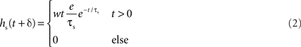
with synaptic weight w (PSC amplitude), time constant τ_s (time to peak), and delay δ. Thus, the synapse acts as a second-order low-pass filter with transfer function

characterized by its corner frequency f_s = 1/(2πτ_s). For f = f_s, the amplitude of the PSC transfer function has dropped by a factor 1/2, i.e., H_s(f_s) = H_s(0)/2. For comparison between the second- order synaptic and the 1st-order firing-rate transfer function (see below), it is convenient to define the synaptic cutoff frequency as 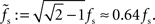At this frequency, the amplitude of (3) has decayed by a factor . The voltage response (PSP) of the neuron to a single presynaptic spike arriving at time t = −δ is given by

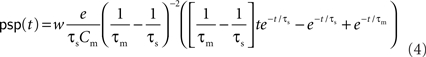
(Rotter and Diesmann, 1999). For a given synaptic weight w, the PSP maximum PSP_max(w) can be calculated numerically. We refer to the minimal weight w_crit which causes the PSP to reach the threshold, i.e., for which PSP_max(w_crit) = V_th, as the critical weight. The dependence of w_crit on the synaptic and membrane time constants τ_s and τ_m, respectively, is shown in Figure 2. In this work, all synaptic weights are considered relative to w_crit, i.e., w_r = w/w_crit. The present study is restricted to purely excitatory synapses with w > 0.

TABLE 1

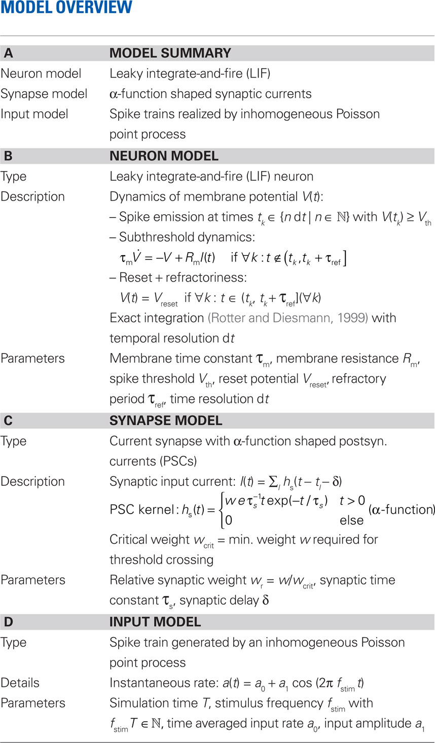
Table 1. Overview of the model.

The input spike train to the cell is modeled as a realization of an inhomogeneous Poisson point process with sinusoidal rate a(t) with oscillation frequency f_stim∈[1,1000] Hz, mean rate a₀ ∈[0,100] s⁻¹ and modulation depth a₁ ∈[0,100] s⁻¹ (see Figure 1). For data analysis, only data for a₁ < a₀ were taken into account (non-rectified input). To test the predictive power of the rate model we also applied other, non-sinusoidal, stimuli, e.g., firing-rate steps (see Section 3.5). Realizations of inhomogeneous Poisson processes with rate function a(t) were generated by applying the time-rescaling theorem (see Brown et al., 2001, and references therein), i.e., by first drawing spike times s_i from a homogeneous Poisson process with unit rate and then, in a second step, applying the inverse t_i = Λ^–1(s_i) of the cumulative rate function 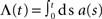to each event time s_i of the realization (see e.g., Devroye, 1986; Nawrot et al., 2008; Cardanobile and Rotter, 2010).

FIGURE 1

Figure 1. Sketch of the setup. A leaky integrate-and-fire (LIF) neuron receives spike trains generated by a Poisson point process with sinusoidal rate of mean a₀ and modulation amplitude a₁. The synapse is modeled as a current kernel (PSC) with amplitude w. The response firing rate is characterized by its mean r₀, amplitude r₁ and phase φ.

FIGURE 2

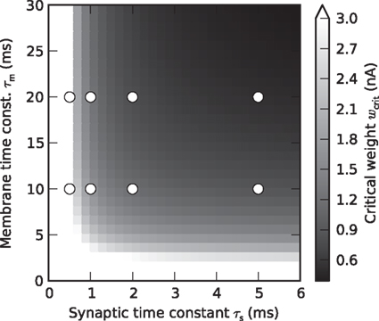
Figure 2. Critical synaptic weight. Dependence of the critical synaptic weight w_crit (gray scale) on the synaptic and membrane time constants τ_s and τ_m, respectively. Symbols mark values of τ_s and τ_m used in the simulations.

A detailed description of the neuron, synapse and input model can be found in Table 1 (Nordlie et al., 2009). Simulations were performed using the exact-integration method presented in (Rotter and Diesmann, 1999) and implemented in NEST (Gewaltig and Diesmann, 2007) with a time resolution of dt = 0.1 ms. The simulation time was set to T = 2²⁰ dt ≈ 105 s. The parameters V_th, V_reset, τ_ref, C_m, and δ were kept constant throughout the whole study. Unless stated otherwise (Sections 3.4 and 3.5), default values τ_s = 2 and τ_m =10 ms were used for the synaptic and membrane time constants, respectively. Response spike trains were recorded for a wide range of synaptic weights w and stimulus parameters a₀, a₁, f_stim. The parameter settings are summarized in Table 3.

2.2 Characterization of Response Properties

For each parameter set, we constructed a discretized version of the instantaneous firing rate r(t) (spike density; t ∈{k dt|k = 0,1,2,…,T/dt}) by counting the number of response spikes in each time interval [t,t + dt) and normalized it by dt = 0.1 ms. As dt < τ_ref, the spike count in each bin was either 0 or 1. For each stimulus frequency f_stim, we obtained the time averaged firing rate r₀ = T⁻¹R(0) and the response amplitudes r_k(f_stim) = 2T⁻¹|R(k f_stim)| (k ∈ {1,2}) from the (finite-time) Fourier transform of r(t). For the principal harmonics (k = 1), we also measured the phase φ of R(f) at frequency f_stim. The discrete Fourier transform was computed using the Fast Fourier Transform (FFT; Press et al., 1992) implemented in Python/Numpy⁵. To improve the efficiency of the FFT, the simulation time T was chosen such that the number of time steps T/dt = 2²⁰ is an integer power of 2. Further, to ensure that the stimulus frequencies f_stim were represented in the discrete Fourier transforms, they were chosen such that T always contained an integer number of stimulus periods, i.e., T f_stim ∈ ℕ.

Assuming Poissonian spike-train statistics, the variance Δ²r = 4r₀/T of the amplitude r₁ is determined by the expected firing rate r₀ and the observation time T (Papoulis and Pillai, 2002). This holds for both homogeneous and inhomogeneous Poisson processes and for all frequencies f. To evaluate whether a measured modulation amplitude r₁ significantly differs from zero (homogeneous case), we computed the z-score for each amplitude r₁. For a homogeneous Poisson process, the probability of observing an amplitude r₁ with z > 2 is less than 5% (values above the horizontal dashed lines in Figures 4A,C,E).

The stationary response to constant input (f_stim = 0, a₁ = 0) is described by the activation function r₀ = g(a₀), measured on a grid a₀ ∈ {0,2,…,100} s⁻¹ (see Figure 3). For the prediction of population-averaged responses (see Section 3.5), a continuous representation of the activation function was obtained by linear interpolation. To characterize the response to nonstationary input (f_stim > 0, a₁ > 0), we computed the complex transfer function

from the measured response amplitude r₁(f_stim) and phase φ(f_stim) (see Figure 4). To obtain a more compact description of the response characteristics, we fitted the transfer function

of a first-order low-pass filter with cutoff frequency f_c, low-frequency gain γ and constant (frequency independent) delay d to the measured transfer function H₀(f) by minimizing the Euclidean distance

between the data and the model in the complex plane for all stimulus frequencies f_i (least-square fit; Levenberg–Marquardt algorithm; see Figure 4). In the time domain, (6) corresponds to a delayed exponential kernel

with a time constant τ = 1/(2π f_c). As a measure of the robustness of the fit, we computed the standard deviation of fit parameters f_c, γ, and d (error bars in Figure 5) obtained from an ensemble (100 trials) of surrogate data, generated by drawing random numbers from a complex Gaussian distribution with mean and standard deviation for each stimulus frequency f_stim. For further analysis, only parameter sets {w_r, a₀, a₁, τ_s,τ_m} with z-scores z(f_stim) ≥ 2 for all f_stim ≤ 2f_c were taken into account.

FIGURE 3

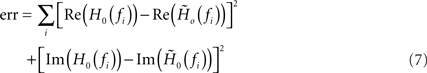
Figure 3. Weight dependence of the stationary response (a₁ = 0). (A) Dependence of the response firing rate r₀ on the constant input rate a₀ (activation function) for relative synaptic weights w_r ∈ {0.2, 0.3,…1.5} (cf. numbers on the right margin). (B) Dependence of the transfer ratio r₀/a₀ (gray scale) on the input rate a₀ and the synaptic weight w_r.

FIGURE 4

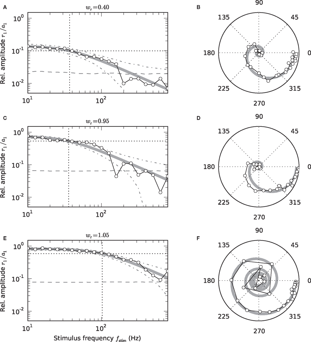
Figure 4. Low-pass characteristics of the nonstationary response (a₁ > 0). Frequency dependence of the transfer-function amplitude r₁ (f_stim)/a₁ (A,C,E), and transfer function H₀(f) in the complex plane (B,D,F: radius = amplitude; angle = phase) for w_r = 0.4 (A,B), 0.95 (C,D), 1.05 (E,F). Symbols represent measured responses. Thick gray curves show fitted 1st-order low-pass filters (see Eq. (6)). Vertical dotted lines in A, C, and E mark fitted cutoff frequencies f_c. Dashed horizontal lines in A,C,E represent 2SD of the amplitude of a homogeneous Poisson process with rate r₀. Dash-dotted curves mark mean ± 2 SD of the amplitude of a sinusoidal Poisson process with expected amplitude r₁(f_stim) given by the first-order low-pass model (thick gray curve). (A–F) a₀ = 42 s^-1, a₁ = 30 s⁻¹.

FIGURE 5

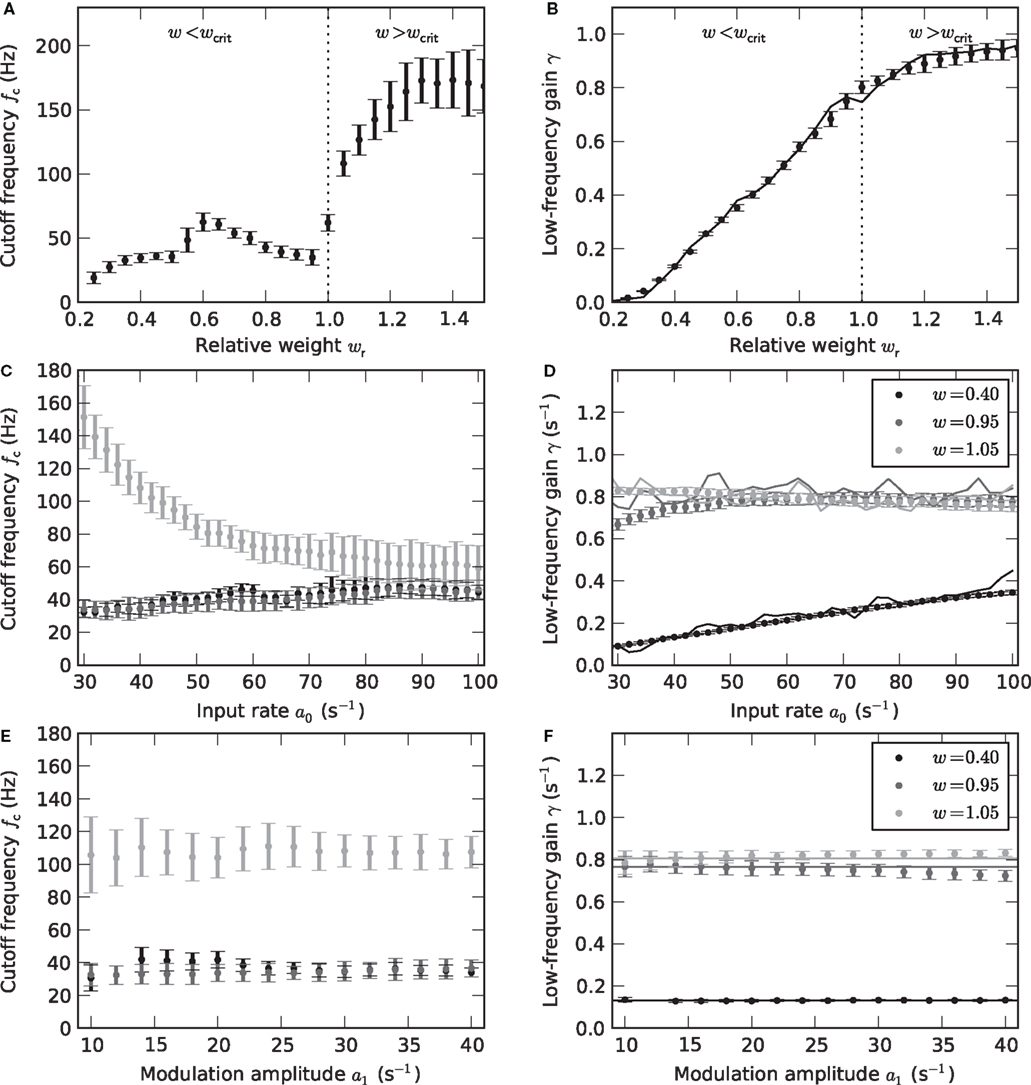
Figure 5. Weight and input dependence of the rate transfer function. Dependence of the cutoff frequency f_c (left column) and the low-frequency gain γ (right column) on the relative synaptic weight w_r (A,B), the mean input rate a₀ (C,D) and the input amplitude a₁ (E,F). Solid curves in the right column show the slope g´ (a₀) of the activation function at the working point a₀. Dotted vertical lines in (A,B) mark w = w_crit. In (C–F), data for w_r = 0.4 (black), 0.95 (dark gray) and 1.05 (light gray) are shown. Error bars represent mean ± standard deviation. (A,B: a₀ = 40 s⁻¹, a₁ = 30 s⁻¹. C,D: a₁ = 30 s⁻¹. E,F: a₀ = 40 s⁻¹.)

Across wide parameter regions, we found that (6) provides a reasonable fit of the measured amplitudes and phases. We do not imply, however, that the first-order low-pass filter is the optimal description. We mainly use it as a tool to extract transfer features like the cutoff frequency and the low-frequency gain, which in turn can be used to construct a firing-rate model (see Section 2.3). In Section 3.5, we demonstrate that such a model can be used to reliably predict population responses to non-sinusoidal stimuli.

A summary of the data analysis can be found in Table 2.

TABLE 2

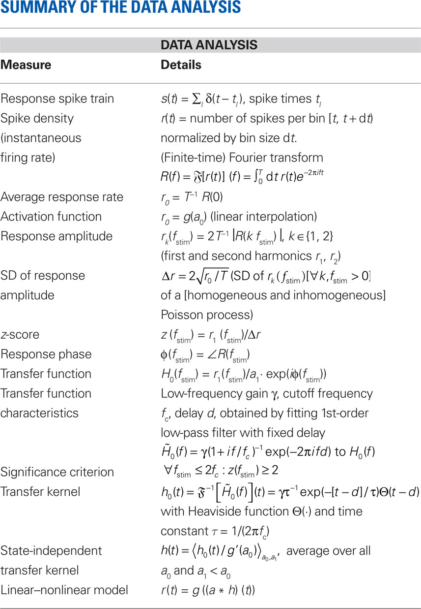
Table 2. Summary of the data analysis.

TABLE 3

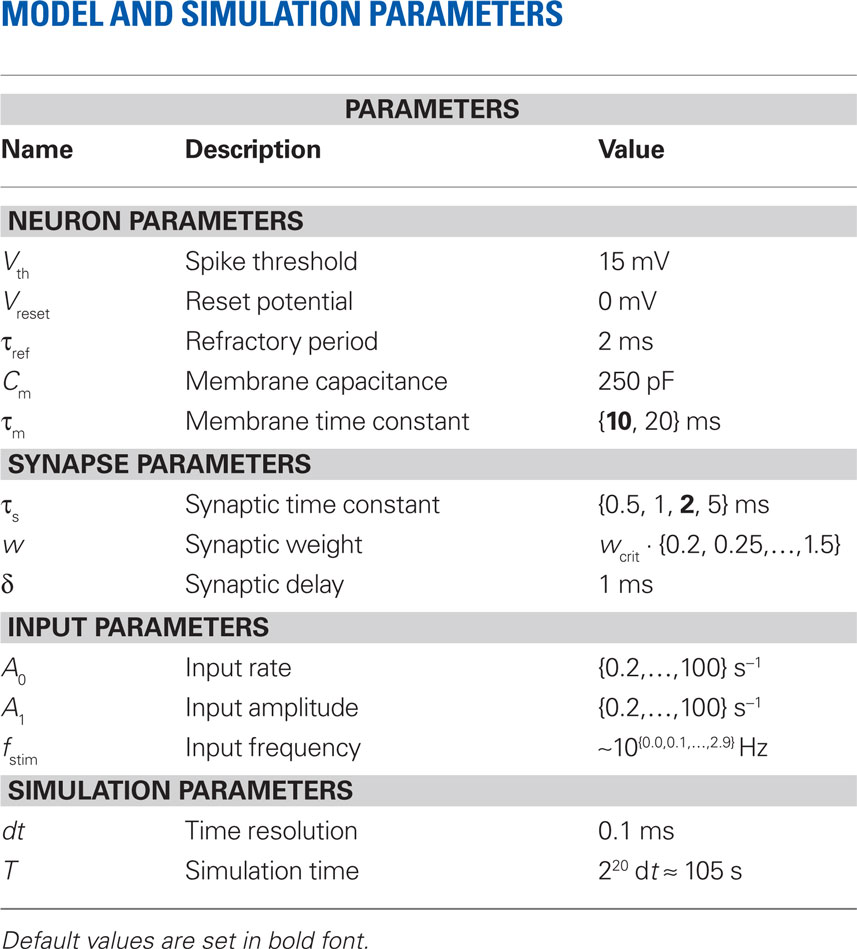
Table 3. Curly brackets {…} represent ranges of values used in the simulations.

2.3 Linear–Nonlinear Model

The linear description (1) is frequently extended by combining a state-independent linear kernel h(t) with a nonlinear activation function g(·), resulting in a linear–nonlinear integral-equation model

An alternative approach based on Wiener kernels is presented, for example, in (Sakai, 1992). Firing-rate models are often expressed in terms of differential equations (e.g., Wilson and Cowan, 1972). Indeed, for an exponential kernel h(t) (which corresponds to the first-order low-pass filter (6)) and with u(t) = (a ∗ h)(t) and , Eq. (9) is equivalent to

(see Nordbø et al., 2007, and references therein)⁶. Note, that from this point of view the dynamical variable u(t) corresponds to the linear response of the firing rate. It describes neither the average synaptic input nor the membrane potential. A priori, the kernel h(t) can therefore not be interpreted as the synaptic or membrane filter. For the mathematical and numerical analysis, the differential form (10) of the rate model is often more convenient. The integral form (9) represents a more general description for arbitrary linear kernels h(t).

For small perturbations Δa(t) of a stationary working point a₀, (9) should be to leading order identical to (1) (for x(t) = a(t)). As a consequence, the dependence of the transfer kernel h₀(t) on the choice of the working point a₀ is determined by the slope g′(a₀) = dg(a₀)/da₀ of the activation function at this point, i.e.,

As we will show in Section 3.2, for a wide range of parameters the dependence of the filter kernel h₀(t) on the working point a₀ is indeed given by the slope g′(a₀) of the activation function alone, i.e., the extracted kernel h(t) = h₀(t)/g′(a₀) is independent of the applied stimulus. We therefore pool our results in this region of the parameter space by averaging h(t) over all a₀ and all a₁ < a₀. Based on the kernel h(t) obtained this way and the measured activation function g(a₀), we set up a linear–nonlinear model (9) which allows us to compute the responses r(t) to arbitrary stimuli a(t) (see Section 3.5).

The model (9) was extracted from the Fourier transform of the spike response of a single neuron. This corresponds to an analysis of the period-averaged signal. Provided the responses in consecutive stimulus periods are independent, period averaging is equivalent to averaging across independent trials or across a population of independent neurons. In Section 3.5, we test to what extent the rate model extracted from a single neuron by period averaging can predict the population-averaged spike response of an ensemble of LIF neurons receiving input spike trains with non-sinusoidal firing rate.

3 Results

3.1 Stationary Response

In the present study, the synaptic input is purely excitatory. For stationary inputs, the output rate r₀ therefore increases monotonously with the input rate a₀ (Figure 3A). For subcritical synaptic weights w_r < 1, the postsynaptic neuron has to integrate a number of presynaptic events to reach the threshold (cf. Usrey et al., 1998, in the context of the retina-LGN system). In consequence, the output rate r₀ is smaller than the input rate a₀. As with increasing input rate a₀ more and more charge is accumulated, the transfer ratio r₀/a₀ increases with a₀ (Figure 3B). The activation function r₀ = g(a₀) is therefore concave in this regime. At the critical weight w_r = 1, an isolated input spike causes a depolarization of the postsynaptic cell which just reaches the threshold V_th. For w_r ≥ 1, one could therefore expect that each input spike is transferred, such that r₀/a₀ = 1. Due to refractoriness, however, a fraction of input spikes is lost. This fraction increases with the input rate a₀ because the number of short inter-spike intervals increases. In consequence, the activation function becomes convex for larger a₀, i.e., the transfer ratio r₀/a₀ decreases with a₀. For strong weights w_r > 1, fewer input spikes are lost because the postsynaptic currents are extended in time (alpha-PSCs). Even if an input spike arrives within the refractory period, the resulting PSC can still be suprathreshold after the neuron has recovered. For the same reason, the transfer ratio can even become larger than one for larger synaptic time constants Ƭ_s (see for example Figures 8L,O).

As shown in Figure 3B, the transfer ratio r₀/a₀ is non- continuous at the critical weight w_r = 1. This is most apparent for small and moderate input rates a₀. Even if the synaptic weight is only slightly smaller than the critical weight, the transfer ratio is considerably smaller than 1. At the critical weight, it jumps to values close to 1.

3.2 Nonstationary Response

As illustrated in Figure 4, the response to a time-varying input rate can be well described by a linear first-order low-pass filter (6) with cutoff frequency f_c, low-frequency gain γ and fixed delay d. Both the cutoff frequencies f_c and the low-frequency gain γ are larger for supercritical synaptic weights w > w_crit as compared to subcritical ones. Note that the cutoff frequency for an intermediate weight w_r = 0.4 (A) is almost identical to the cutoff frequency for a weight w_r = 0.95 which is close to the critical weight (C). At the critical weight, the cutoff frequency jumps to higher values (E, w_r = 1.05). The dependence of f_c and γ on the synaptic weight is explicitly shown in Figures 5A,B (for a₀ = 40 and a₁ = 30 s⁻¹). For subcritical weights w < w_crit, the rate-transfer cutoff frequency f_c is smaller than or close to the cutoff frequency of the synaptic filter (alpha-kernel with time constant τ_s = 2 ms; see Section 2.1). At the critical weight w_r = 1, f_c jumps to high values above 100 Hz. In contrast to this sharp transition in the cutoff frequency, the low-frequency gain γ increases continuously with w_r. For large weights, it approaches values close to one. Here, the response modulation at small frequencies is almost as large as the modulation in the input rate. In agreement with (11), the low-frequency gain γ is well explained by the slope g′(a₀) of the activation function at the working point a₀ (thin solid line in Figure 5B).

Figures 5C–F depict the dependence of the filter characteristics f_c and γ on the mean a₀ and modulation depth a₁ of the input signal. For subcritical weights w_r < 1, the cutoff frequency f_c is approximately independent of both a₀ and a₁ (Figures 5C,E). Only for small synaptic time constants τ_s, the cutoff frequency f_c slightly increases with a₀ (data not shown). For supercritical weights w_r > 1, we observe a decrease in f_c with a₀ (light gray curve in Figure 5C). The low-frequency gain γ (Figures 5D,F) is in good approximation determined by the slope g′(a₀) of the activation function evaluated at the input rate a₀ (thin solid curves in Figures 5D,F).

For a linear–nonlinear model (9), the kernel h(t) is given by h₀(t)/g′(a₀) (see Section 2.3). For subcritical weights, we observe that h(t) is approximately independent of both a₀ and a₁. An important prerequisite for a model which does not depend on the input a(t) is thereby fulfilled. For the construction of the firing-rate model (9), we therefore pooled the data by averaging h(t) over all a₀ and all a₁ < a₀. Although the cutoff frequency depends on the choice of the working point a₀ for supercritical weights, we also attempt the same strategy here. In Section 3.5, we will test the performance of this model for non-sinusoidal stimuli.

3.3 Linearity of the Response

Strictly speaking, measuring the linear response H₀(f) of a nonlinear system at a working point a₀ requires infinitesimally small perturbations. In practice, it is a priori unclear which perturbation amplitudes can be considered sufficiently small. In the framework used here, we can quantify this by analyzing the frequency contents of the response r(t). In the linear regime, a sinusoidal stimulus of frequency f_stim will give rise to a single peak in the response amplitude spectrum at the same frequency f_stim. Leaving the linear regime is in general accompanied by the occurrence of higher harmonics. To map the linear regime, we therefore compared the amplitudes of the principal and second harmonics r₁ and r₂, respectively, for all neuron and stimulus parameters. Figure 6 shows the results for a mean input rate a₀ = 40 s⁻¹ and a modulation frequency f_stim = 10 Hz (similar results were obtained for other stimulus frequencies and input rates). In Figure 6A, the amplitudes of the first two harmonics are shown for three different synaptic weights. For sufficiently small input amplitudes a₁, the amplitude r₂ of the second harmonics does not exceed the noise level. Note, that r₂ is never exactly zero because of a finite observation time T (see Section 2.2). The ratio r₁/(r₁ + r₂) shown in Figure 6B is thus never exactly 1. For weights w_r > 0.6 and intermediate input amplitudes a₁, the rate transfer is approximately linear. For synaptic weights w_r < 0.6, we observe an increase in r₂ for larger modulation depths (Figure 6B) which is due to a rectification of the response modulation (r₁ ≥ r₀; see dotted curves in Figure 6B).

FIGURE 6

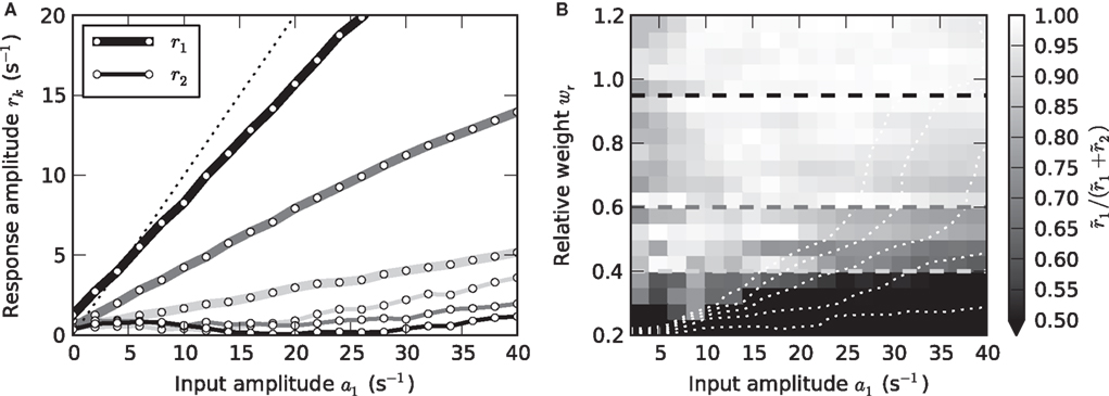
Figure 6. Linearity of rate transfer. (A) Dependence of the amplitude r_k of the first two Fourier components (k = 1, 2, cf. legend) on the stimulus amplitude a₁ for w_r = 0.4 (light gray), 0.6 (dark gray), and 0.95 (black). Dotted line represents diagonal r_k = a₁. (B) Relative amplitude of the principal response mode (after offset subtraction and rectification, i.e., ) as function of the synaptic weight w_r and the stimulus amplitude a₁. Dashed horizontal lines mark synaptic weights shown in (A). (A,B) a₀ = 40 s⁻¹, f_stim = 10 Hz. White dotted curves mark regions where r₀ ≤ r₁ (iso-contour lines of r₀/r₁ at values 1,0.9,0.8,0.7,0.6 [from left to right]).

3.4 Dependence on Synaptic and Membrane Time Constants

At first sight, one might expect that the tracking speed of a population of neurons is limited by the low-pass filter properties of the neuronal membrane, i.e., the membrane time constant τ_m. Previous studies (e.g., Gerstner, 2000) have however shown, that the cutoff frequency of the rate transfer is rather determined by the synaptic time constant τ_s. Here, we test this for a number of time constants τ_s ∈ {0,5,1,2,5} and τ_m ∈ {10,20} ms. In Figure 7A, the cutoff frequency f_c of the rate transfer normalized by the cutoff frequency of the synaptic kernel is plotted as a function of the relative synaptic weight w_r for different synaptic and membrane time constants τ_s and τ_m, respectively. For the whole range of tested synaptic weights, the cutoff frequencies do not significantly differ for the two considered membrane time constants τ_m = 10 ms (solid curves) and 20 ms (dashed curves). In the subcritical regime w_r < 1, the firing-rate cutoff frequency f_c is close to or slightly smaller than the synaptic cutoff . The ratio is approximately independent of τ_s. Thus, the cutoff frequency f_c of the rate transfer is indeed bounded from above by the synaptic cutoff frequency . For supercritical weights w_r > 1, f_c depends on in a nonlinear (but still monotonous) fashion. For small τ_s, the cutoff frequency of the rate transfer can considerably exceed the synaptic cutoff frequency. In other words, the time constant τ = 1/(2πf_c) can be much smaller than the synaptic time constant τ_s.

FIGURE 7

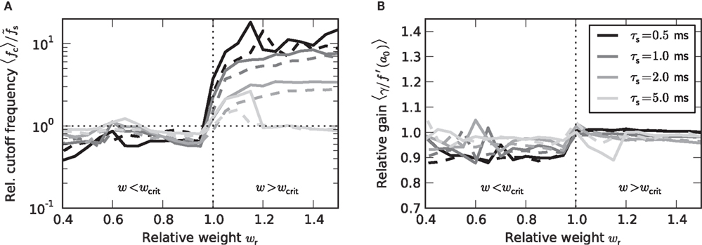
Figure 7. Dependence of the rate transfer function on the synaptic and membrane time constants. Weight dependence of the relative cutoff frequency (A) and the normalized low-frequency gain 〈γ/g′(a₀)〉 (B) for different synaptic time constants τ_s ∈ {0.5,1.0,2.0,5.0} ms (from black to light gray; see legend), i.e., , and membrane time constants τ_m = 10 ms (solid) and 20 ms (dashed). Dotted horizontal line in (A) marks . Dotted vertical lines in (A) and (B) mark w = w_crit. Data represent averages (〈·〉) over all a₀ and a₁ < a₀.

As shown in Figure 7B, the low-frequency gain γ is, as a good approximation, given by the slope g′(a₀) of the activation function, independently of the choice of the time constants τ_s and τ_m, and the synaptic weight w_r.

3.5 Test of the Linear–Nonlinear Model

By systematically varying the parameters f_stim, a₀ and a₁ of the sinusoidal input rate, we obtained an activation function g(·) (Figure 3) and a linear state-independent transfer kernel h(t) (Figures 4, 5, and 7) for each parameter set {w,τ_s,τ_m}. With these ingredients we set up firing-rate models of the form (9). The model extraction is based on the period-averaged responses of a single neuron to sinusoidal inputs, a procedure which is often applied in experimental neuroscience. Provided the spike responses in consecutive stimulus periods are independent the resulting firing-rate model should also yield accurate predictions for the instantaneous population-averaged response of an ensemble of independent (unconnected) neurons. Figure 8 illustrates that this is in fact the case for subcritical synaptic weights w_r < 1 (Figures 8A–I): here, the population-averaged step response of an ensemble of 50000 independent LIF neurons (black curves) is well described by the linear–nonlinear model (gray curves). Both the time constants τ = 1/(2πf_c) of the rate dynamics (9) and the stationary response rates are correctly predicted. Similarly good agreement between the rate-model predictions and the results of direct simulation was obtained for a variety of other test stimuli.

FIGURE 8

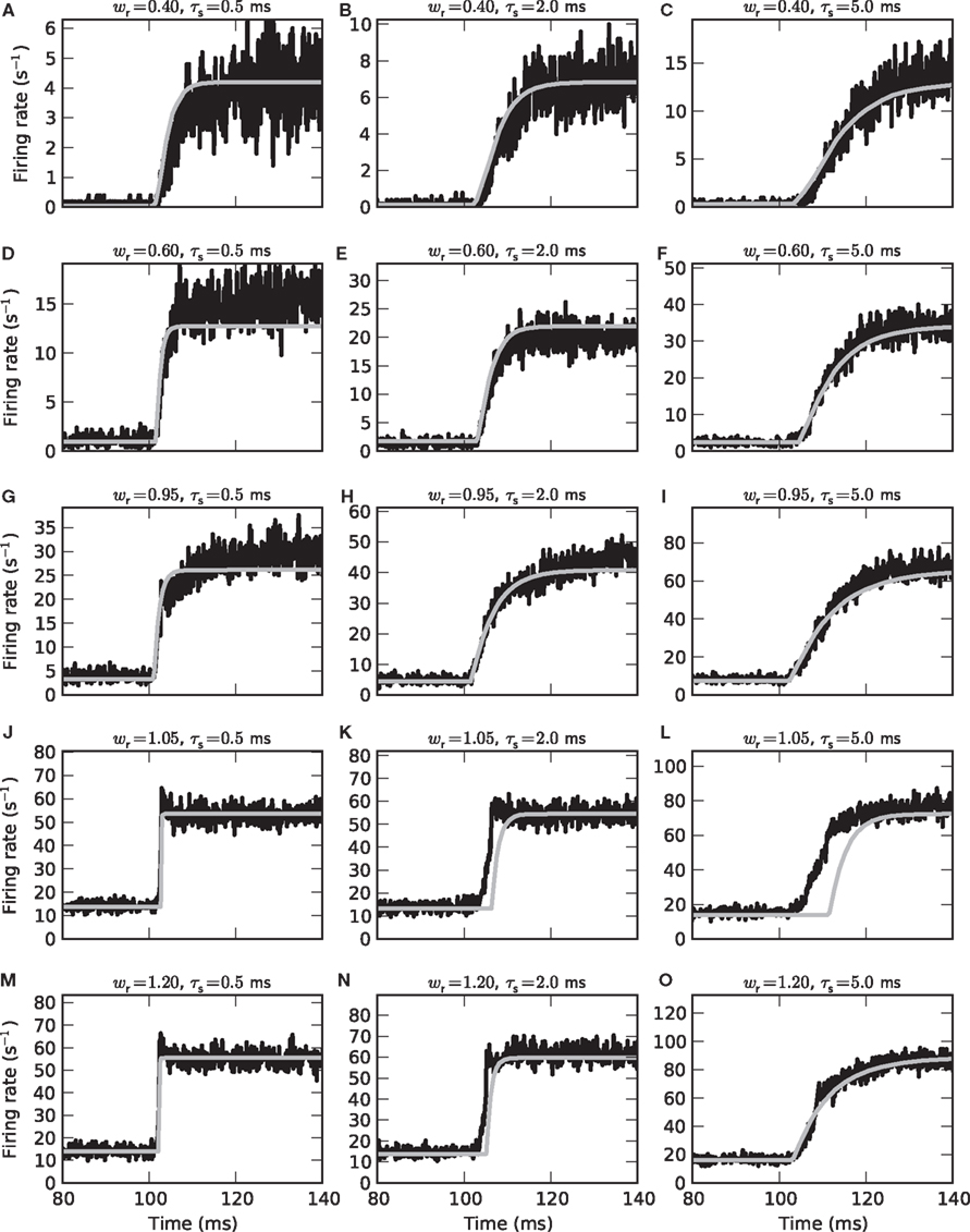
Figure 8. Population-averaged step response. Firing rate r(t) in response to an instantaneous increase in the input firing rate a(t) at time t = 100 ms from 15 to 65 s⁻¹ for different synaptic weights w_r = 0.4 (A–C), 0.6 (D–F), 0.95 (G–I), 1.05 (J–L), and 1.2 (M–O) and time constants τ_s = 0.5 (left column), 2 (middle column) and 5 ms (right column). Comparison between direct simulation results (black curves; population-averaged response of 50000 neurons, bin size dt = 0.1 ms) and prediction of the linear–nonlinear model (9) (gray curves) with measured activation function g(a₀) and transfer kernel h(t) (averaged over all a₀ and a₁< a₀).

In a few cases, we observe some subtle differences between model predictions and simulation results: For small τ_s and subcritical weights, the time constants of the model are slightly underestimated (see e.g., Figure 8A). For supercritical weights w_r > 1, the population-averaged step response sometimes exhibits an overshoot immediately after the jump in the input rate which is not captured by the model (Figures 8J,M). Further, the model overestimates the rate transmission delay d in some cases (Figures 8K,L,N). It is likely that these deviations for small synaptic time constants or supercritical weights are a result of the dependence of the cutoff frequency on the choice of the working point a₀ (see Figure 5C). The averaging strategy leading to the state-independent kernel h(t) ignores this dependence.

4 Discussion

In the present study, we investigated how LIF neurons transmit presynaptic time-varying firing rates to the output rate in a period- or population-averaged sense. In contrast to earlier studies, we focused on a regime where the synapses have moderate or large synaptic weights and where the average input rates are relatively low. The response properties were characterized by measuring the activation function g(a₀), i.e., the response r₀ to constant input rates a₀, and the transfer function H₀(f) describing the transmission of time-varying rate perturbations in the vicinity of a working point a₀. Both concepts, the activation function and the transfer function, were used to set up a firing-rate model which was evaluated by comparing its predictions with simulation results for non-sinusoidal test stimuli.

In agreement with previous work (Sirovich, 2008), we found that even for strong synapses only a fraction of the input spikes is transmitted. Only for (presumably) unrealistically large synaptic weights above a critical value w_crit, the transfer ratio r₀/a₀ approaches or even exceeds one. We have observed this behavior for both stationary and nonstationary inputs.

In the diffusive regime, i.e., for weak synapses, different transfer scenarios have been described in the literature for different neuron and stimulus models. All previous studies predict some sort of low-pass behavior (at least if one takes into account that incoming spikes are low-pass filtered by the synapses). We observe similar behavior for large synaptic weights. If the synapses are so strong that a single isolated input spike can reliably cause a response spike in the postsynaptic neuron, i.e., for w > w_crit, one would expect that any signal carried by the presynaptic spikes can be transmitted – no matter what its frequency contents is and independently of the synaptic filter properties. Both weights larger than w_crit and infinitesimally small weights are unrealistic for most biological neural systems. It is tempting to interpolate between these two extreme cases and assume that the ability of a neuron population to track fast stimuli gradually increases with the synaptic strength w. In fact, Helias et al. (2010) have recently shown that for finite synaptic weights the population response of an ensemble of integrate-and-fire neurons exhibits an instantaneous component which gradually increases with the synaptic weight. The analysis presented in (Helias et al., 2010) is however still restricted to small synaptic weights. For strong but subcritical weights w < w_crit, we found that the cutoff frequency f_c of the rate transfer is bounded from above by the synaptic cutoff frequency . Only for supercritical weights w > w_crit, the tracking speed of the population can be significantly increased. In agreement with earlier work (e.g., Gerstner, 2000), our data suggest that the cutoff frequency f_c of the rate transfer does not depend on the choice of the membrane time constant.

In most previous studies, the stimulus is treated as a modulation of the distribution of postsynaptic somatic currents. In our study, in contrast, the stimulus is represented by a modulation in the presynaptic firing rate. Here, the effective transfer function is a combination of the neuronal (the current-to-rate transfer) and the synaptic filtering (rate-to-current transfer). For correlated noise, it has been shown that ensembles of LIF neurons can faithfully transmit fast modulations in the mean or the variance of the input current (see e.g., Brunel et al., 2001; Lindner and Schimansky-Geier, 2001): the response amplitudes remain finite even at high frequencies. In this case, the net filtering at high frequencies is governed by the synaptic kernel h_s(t) alone. For alpha-function shaped synaptic currents (as used in this study), one would therefore expect second-order low-pass characteristics with response amplitudes decaying as 1/f² at high frequencies (see (3)). Note, however, that this result refers to the diffusion limit, i.e., infinitesimal synaptic weights. For non-diffusive regimes, the shape of the neuronal transfer function is unknown. Here, we for simplicity describe the data by a first-order low-pass filter. For most parameters, this results in reasonable fits (see, for example, Figure 4). In practice, however, the high-frequency response can easily be affected by noise: due to the stochastic nature of the input spike trains and finite observation times, small amplitudes are in general overestimated. This may lead to a flattening of the transfer function. Here, we do not address the exact shape of the transfer function at high frequencies. Instead, we restrict this study to a description of the cutoff frequency and the low-frequency gain in order to design a simple firing-rate model. We tested that these characteristics are rather robust against the choice of the transfer function⁷. Since the work of Wilson and Cowan (1972), firing-rate models with exponential kernels (i.e., first-order low-pass filters) have become a standard tool in neuroscience⁸. In the present study, we show that the presence of strong synapses does not necessarily disqualify such models. For an ensemble of unconnected LIF neurons, we demonstrated that a simple 1st-order model yields accurate predictions of the population-averaged response for a wide range of stimulus, neuron, and synapse parameters. For recurrent systems, however, the exact shape of the rate transfer function at high frequencies can be crucial: Nordbø et al. (2007), for example, have shown that the shape of the rate-transfer kernel determines the stability of persistent states in neural-field models. Solutions which are stable for exponential kernels can become unstable for alpha-function kernels. In future studies, the performance of the rate model extracted here therefore needs to be tested under recurrent conditions.

The approach presented in this study can in principle be applied to any nonlinear system. In general, this leads to transfer functions which depend on the choice of the working point (a₀, r₀) in a non-trivial way. For large but subcritical synaptic weights and not too small synaptic time constants, we observed that the normalized rate-to-rate transfer function H(f) = H₀(f)/g′(a₀) is approximately independent of the working point and mainly determined by the synaptic filter. Here, a simple linear–nonlinear model r(t) = g((a ∗ h (t)) with a state-independent kernel h(t) yields accurate predictions of the population-averaged firing rate. In accordance with previous studies (e.g., Knight, 1972a; Brunel et al., 2001; Lindner and Schimansky-Geier, 2001; Mattia and Del Giudice, 2002), we found that for small synaptic time constants τ_s the cutoff frequencies f_c increase with the firing rate. If the synaptic cutoff frequency is small compared to the firing rate r₀ (i.e., for larger synaptic time constants), the synaptic filter seems to dominate. If is large, a precise prediction of the response rate would require a model which takes the state-dependence of the transfer kernel explicitly into account. As shown in Figure 8, the predictive power of the reduced model with a state-independent kernel is however acceptable even for fast synapses and low firing rates.

For small synaptic weights, previous studies have shown that the characteristics of the transmission of time-varying input currents to output rates crucially depends on the properties of the neuron model (Knight, 1972a; Fourcaud-Trocmé et al., 2003; Naundorf et al., 2005). Our study is restricted to the LIF model. Future work needs to show how more (or less) biologically realistic neuron models alter our findings on the transmission of input firing rates (rather than input currents) with finite synaptic weights. In our and in most previous studies on the transfer characteristics of neuron ensembles, synapses are modeled as static kernels describing the PSC. The effect of conductance-based (see e.g., Kuhn et al., 2004, and references therein) or dynamical synapses (Tsodyks et al., 1998), for example, on the firing-rate filter properties of a neuron ensemble is so far unclear. Another restriction in our work is the neglect of inhibitory inputs. Pressley and Troyer (2009) recently pointed out that the rate transfer of a population of perfect integrate-and-fire neurons depends on the interplay between presynaptic excitation and inhibition.

A number of experimental studies has systematically characterized the stationary (e.g., Arsiero et al., 2007) and nonstationary response properties (Köndgen et al., 2008; Boucsein et al., 2009) of populations of neurons in vitro. As we have suggested here, the combination of both transfer characteristics can – in principle – lead to powerful firing-rate models which allow the description of neuronal activity on a macroscopic scale. We (and others) pointed out that the transfer characteristics are to a large extent determined by the properties of the synapses. The above-mentioned experimental studies are based on direct somatic current injections. The role of the synapses has thus been ignored so far. The controlled stimulation of a large number of individual synapses in in vitro (and in vivo) experiments is difficult. Recent developments in experimental techniques (e.g., Boucsein et al., 2005), however, give hope that this problem may be overcome in the near future.

Conflict of Interest Statement

The authors declare that the research was conducted in the absence of any commercial or financial relationships that could be construed as a potential conflict of interest.

5 Acknowledgments

We thank Hans Ekkehard Plesser and the two reviewers for constructive discussions and valuable comments on the manuscript. We acknowledge partial support by the Research Council of Norway (eNEURO, NOTUR) and the Honda Research Institute Europe. Simulations and data analysis were carried out using the NEST simulation tool⁹ and Python¹⁰.

Footnotes

1. ^Also called “linear response function” or “susceptibility.”
2. ^ denotes the Fourier transform of the function h(t).
3. ^The subscript “0” indicates that the impulse response and the transfer function in general depend on the choice of the working point .
4. ^The “∗” operator denotes the convolution integral:
5. ^http://numpy.scipy.org
6. ^In fact, Eq. (9) can be transformed to a set of differential equations for the whole family of exponential kernels
7. ^Fitting of a second-order filter to the data led to similar result as the first-order model (data not shown).
8. ^For exponential kernels h(t), the linear–nonlinear model (9) can be transformed into a one-dimensional differential Eq. (10). The mathematical and numerical analysis of the model is thereby considerably simplified.
9. ^www.nest-initiative.org
10. ^www.python.org

References

Arsiero, M., Lüscher, H.-R., Lundstrom, B. N., and Giugliano, M. (2007). The impact of input fluctuations on the frequency-current relationships of layer 5 pyramidal neurons in the rat medial prefrontal cortex. J. Neurosci. 27, 3274–3284.

Pubmed Abstract | Pubmed Full Text | CrossRef Full Text

Bannister, A. P., and Thomson, A. M. (2007). Dynamic properties of excitatory synaptic connections involving layer 4 pyramidal cells in adult rat and cat neocortex. Cerebr. Cortex 17, 2190–2203.

CrossRef Full Text

Blomquist, P., Devor, A., Indahl, U. G., Ulbert, I., Einevoll, G. T., and Dale, A. M. (2009). Estimation of thalamocortical and intracortical network models from joint thalamic single-electrode and cortical laminar-electrode recordings in the rat barrel system. PLoS Comput. Biol. 5(3), e1000328. doi: 10.1371/journal.pcbi.1000328.

Pubmed Abstract | Pubmed Full Text | CrossRef Full Text

Boucsein, C., Nawrot, M. P., Rotter, S., Aertsen, A., and Heck, D. (2005). Controlling synaptic input patterns in vitro by dynamic photo stimulation. J. Neurophysiol. 94, 2948–2958.

Pubmed Abstract | Pubmed Full Text | CrossRef Full Text

Boucsein, C., Tetzlaff, T., Meier, R., Aertsen, A., and Naundorf, B. (2009). Dynamical response properties of neocortical neuron ensembles: multiplicative versus additive noise. J. Neurosci. 29, 1006–1010.

Pubmed Abstract | Pubmed Full Text | CrossRef Full Text

Brown, E. N., Barbieri, R., Ventura, V., Kaas, R. E., and Frank, L. M. (2001). The time-rescaling theorem and its application to neural spike train data analysis. Neural Comput. 14, 325–346.

CrossRef Full Text

Brunel, N., Chance, F. S., Fourcaud, N., and Abbott, L. F. (2001). Effects of synaptic noise and filtering on the frequency response of spiking neurons. Phys. Rev. Lett. 86, 2186–2189.

Pubmed Abstract | Pubmed Full Text | CrossRef Full Text

Bruno, R. M., and Sakmann, B. (2006). Cortex is driven by weak but synchronously active thalamocortical synapses. Science 312, 1622–1627.

Pubmed Abstract | Pubmed Full Text | CrossRef Full Text

Cardanobile, S., and Rotter, S. (2010). “Simulation of stochastic point processes with defined properties,” in Analysis of Parallel Spike Trains, eds S. Rotter and S. Grün (Berlin: Springer), 343–382.

Cleland, B., Dubin, M., and Levick, W. (1971). Simultaneous recording of input and output of lateral geniculate neurones. Nat. New Biol. 231, 191–192.

Pubmed Abstract | Pubmed Full Text

Destexhe, A., and Sejnowski, T. J. (2009). The Wilson-Cowan model, 36 years later. Biol. Cybern. 101, 1–2.

Pubmed Abstract | Pubmed Full Text | CrossRef Full Text

Devroye, L. (1986). Non-Uniform Random Variate Generation. New York: Springer-Verlag.

DeWeese, M. R., and Zador, A. M. (2006). Non-gaussian membrane potential dynamics imply sparse, synchronous activity in auditory cortex. J. Neurosci. 26, 12206–12218.

Pubmed Abstract | Pubmed Full Text | CrossRef Full Text

Fetz, E., Toyama, K., and Smith, W. (1991). “Synaptic interactions between cortical neurons,” In Cerebral Cortex, Vol. 9, Chapter 1, ed. A. Peters (New York and London: Plenum Press), 1–47.

Fourcaud, N., and Brunel, N. (2002). Dynamics of the firing probability of noisy integrate-and-fire neurons. Neural Comput. 14, 2057–2110.

Pubmed Abstract | Pubmed Full Text | CrossRef Full Text

Fourcaud-Trocmé, N., Hansel, D., van Vreeswijk, C., and Brunel, N. (2003). How spike generation mechanisms determine the neuronal response to fluctuating inputs. J. Neurosci. 23, 11628–11640.

Gerstner, W. (2000). Population dynamics of spiking neurons: fast transients, asynchronous states, and locking. Neural Comput. 12, 43–89.

Pubmed Abstract | Pubmed Full Text | CrossRef Full Text

Gewaltig, M.-O., and Diesmann, M. (2007). NEST (neural simulation tool). Scholarpedia 2, 1430.

CrossRef Full Text

Helias, M., Deger, M., Rotter, S., and Diesmann, M. (2010). Instantaneous non-linear processing by pulse-coupled threshold units. PLoS Comput. Biol. 6(9), e1000929. doi: 10.1371/journal.pcbi.1000929.

Pubmed Abstract | Pubmed Full Text | CrossRef Full Text

Johannesma, P. I. M. (1968). “Diffusion models for the stochastic activity of neurons,” in Neural Networks: Proceedings of the School on Neural Networks Ravello, June 1967, ed E. R. Caianiello (Berlin: Springer-Verlag), 116–144.

Knight, B. W. (1972a). Dynamics of encoding in a population of neurons. J. General Physiol. 59, 734–766.

CrossRef Full Text

Knight, B. W. (1972b). The relationship between the firing rate of a single neuron and the level of activity in a population of neurons. J. General Physiol. 59, 767–778.

CrossRef Full Text

Köndgen, H., Geisler, C., Fusi, S., Wang, X.-J., Lüscher, H.-R., and Giugliano, M. (2008). The dynamical response properties of neocortical neurons to temporally modulated noisy inputs in vitro. Cerebr. Cortex 18, 2086–2097.

CrossRef Full Text

Kuhn, A., Aertsen, A., and Rotter, S. (2004). Neuronal integration of synaptic input in the fluctuation-driven regime. J. Neurosci. 24, 2345–2356.

Pubmed Abstract | Pubmed Full Text | CrossRef Full Text

Lapicque, L. (1907). Recherches quantitatives sur l’excitation electrique des nerfs traitee comme une polarization. J. Physiol. Pathol. Gen. 9, 620–635.

Lee, A., Manns, I., Sakmann, B., and Brecht, M. (2006). Whole-cell recordings in freely moving rats. Neuron 51, 399–407.

Pubmed Abstract | Pubmed Full Text | CrossRef Full Text

Lefort, S., Tomm, C., Sarria, J. F., and Petersen, C. C. (2009). The excitatory neuronal network of the C2 barrel column in mouse primary somatosensory cortex. Neuron 61, 301–316.

Pubmed Abstract | Pubmed Full Text | CrossRef Full Text

Lindner, B., and Schimansky-Geier, L. (2001). Transmission of noise coded versus additive signals through a neuronal ensemble. Phys. Rev. Lett. 86, 2934–2937.

Pubmed Abstract | Pubmed Full Text | CrossRef Full Text

Mattia, M., and Del Giudice, P. (2002). Population dynamics of interacting spiking neurons. Phys. Rev. E. 66, 051917.

CrossRef Full Text

Naundorf, B., Geisel, T., and Wolf, F. (2005). Action potential onset dynamics and the response speed of neuronal populations. J. Comput. Neurosci. 18, 297–309.

Pubmed Abstract | Pubmed Full Text | CrossRef Full Text

Nawrot, M. P., Boucsein, C., Rodriguez Molina, V., Riehle, A., Aertsen, A., and Rotter, S. (2008). Measurement of variability dynamics in cortical spike trains. J. Neurosci. Methods 169, 374–390.

Pubmed Abstract | Pubmed Full Text | CrossRef Full Text

Nordbø, ø., Wyller, J., and Einevoll, G. T. (2007). Neural network firing-rate models on integral form: Effects of temporal coupling kernels on equilibrium-state stability. Biol. Cybern. 97, 195–209.

Pubmed Abstract | Pubmed Full Text

Nordlie, E., Gewaltig, M.-O., and Plesser, H. E. (2009). Towards reproducible descriptions of neuronal network models. PLoS Comput. Biol. 5(8), e1000456. doi: 10.1371/journal.pcbi.1000456.

Pubmed Abstract | Pubmed Full Text | CrossRef Full Text

Papoulis, A., and Pillai, S. U. (2002). Probability, Random Variables, and Stochastic Processes, 4th Edn. Boston: McGraw-Hill.

Press, W. H., Teukolsky, S. A., Vetterling, W. T., and Flannery, B. P. (1992). Numerical Recipes in C, 2nd Edn. Cambridge: Cambridge University Press.

Pressley, J., and Troyer, T. (2009). Complementary responses to mean and variance modulations in the perfect integrate-and-fire model. Biol. Cybern. 101, 63–70.

Pubmed Abstract | Pubmed Full Text | CrossRef Full Text

Richardson, M. J. E. (2007). Firing-rate response of linear and nonlinear integrate-and-fire neurons to modulated current-based and conductance-based synaptic drive. Phys. Rev. E. 76, 1–15.

CrossRef Full Text

Rotter, S., and Diesmann, M. (1999). Exact digital simulation of time-invariant linear systems with applications to neuronal modeling. Biol. Cybern. 81, 381–402.

Pubmed Abstract | Pubmed Full Text | CrossRef Full Text

Sakai, H. M. (1992). White-noise analysis in neurophysiology. Physiol. Rev. 72, 491–505.

Pubmed Abstract | Pubmed Full Text

Silberberg, G., Bethge, M., Markram, H., Pawelzik, K., and Tsodyks, M. (2004). Dynamics of population codes in ensembles of neocortical neurons. J. Neurophysiol. 91, 704–709.

Pubmed Abstract | Pubmed Full Text | CrossRef Full Text

Sirovich, L. (2008). Populations of tightly coupled neurons: The RGC/LGN system. Neural Comput. 20, 1179–1210.

Pubmed Abstract | Pubmed Full Text | CrossRef Full Text

Song, S., Per, S., Reigl, M., Nelson, S., and Chklovskii, D. (2005). Highly nonrandom features of synaptic connectivity in local cortical circuits. PLoS Biol. 3, 0507–0519. doi: 10.1371/journal.pbio.0030068.

CrossRef Full Text

Tsodyks, M., Pawelzik, K., and Markram, H. (1998). Neural networks with dynamic synapses. Neural Comput. 10, 821–835.

Pubmed Abstract | Pubmed Full Text | CrossRef Full Text

Tuckwell, H. C. (1988). Introduction to Theoretical Neurobiology, Vol. 1. Cambridge: Cambridge University Press.

Usrey, W. M., Reppas, J. B., and Reid, R. C. (1998). Paired-spike interactions and synaptic efficacy of retinal inputs to the thalamus. Nature 395, 384–387.

Pubmed Abstract | Pubmed Full Text | CrossRef Full Text

Wilson, H. R., and Cowan, J. D. (1972). Excitatory and inhibitory interactions in localized populations of model neurons. Biophys. J. 12, 1–24.

Pubmed Abstract | Pubmed Full Text | CrossRef Full Text