Gain modulation by an urgency signal controls the speed–accuracy trade-off in a network model of a cortical decision circuit
- 1 Canadian Institutes of Health Research Group in Sensory-Motor Integration, Department of Physiology, Queen’s University, Kingston, ON, Canada
- 2 Department of Systems Science, Beijing Normal University, Beijing, China
The speed–accuracy trade-off (SAT) is ubiquitous in decision tasks. While the neural mechanisms underlying decisions are generally well characterized, the application of decision-theoretic methods to the SAT has been difficult to reconcile with experimental data suggesting that decision thresholds are inflexible. Using a network model of a cortical decision circuit, we demonstrate the SAT in a manner consistent with neural and behavioral data and with mathematical models that optimize speed and accuracy with respect to one another. In simulations of a reaction time task, we modulate the gain of the network with a signal encoding the urgency to respond. As the urgency signal builds up, the network progresses through a series of processing stages supporting noise filtering, integration of evidence, amplification of integrated evidence, and choice selection. Analysis of the network’s dynamics formally characterizes this progression. Slower buildup of urgency increases accuracy by slowing down the progression. Faster buildup has the opposite effect. Because the network always progresses through the same stages, decision-selective firing rates are stereotyped at decision time.
1 Introduction
Subjects in decision making experiments trade speed and accuracy at will (van Veen et al., 2008). Under otherwise identical conditions, they make faster, less accurate decisions when motivated to favor speed, and make slower, more accurate decisions when motivated to favor accuracy. The speed–accuracy trade-off (SAT) is ubiquitous across decision making paradigms, but while the neural mechanisms underlying decisions are generally well characterized (Gold and Shadlen, 2001; Schall, 2001), the neural basis of the SAT is an open question (Gold and Shadlen, 2002).
Experimental and theoretical work indicates that decisions result from mutual inhibition between neural populations selective for each option of a decision (see Gold and Shadlen, 2007), where intrinsic (recurrent) synapses support the integration of evidence over time (Usher and McClelland, 2001; Wang, 2002). Mutual inhibition ensures that the representation of evidence accumulating in each population comes at the expense of evidence accumulating in the other(s), implementing a subtractive operation (see Smith and Ratcliff, 2004; Bogacz, 2007). This neural framework instantiates a class of algorithms frequently referred to as the drift diffusion model (DDM), known to yield the fastest decisions for a given level of accuracy and the most accurate decisions for a given decision time (see Bogacz et al., 2006). Speed and accuracy can be traded in the DDM by adjusting the level of evidence required for a decision (the decision threshold; Gold and Shadlen, 2002). Empirical studies, however, indicate that decision-correlated neural activity reaches a fixed threshold at decision time (Hanes and Schall, 1996; Roitman and Shadlen, 2002; Churchland et al., 2008). How, then, can the SAT be accomplished by neural populations with a fixed decision threshold?
A convergence of evidence offers an answer. In neuronal networks with extensive intrinsic connectivity, integration times are determined by network dynamics (Usher and McClelland, 2001; Wang, 2002, 2008; Wong and Wang, 2006). Control of these dynamics is therefore a potential means of trading speed and accuracy. Gain modulation offers a means of control, where the magnitude of the neural response to sensory evidence changes as a function of a second input signal (Salinas and Thier, 2000; Salinas and Sejnowski, 2001). We propose that the neural encoding of elapsed time (Leon and Shadlen, 2003; Janssen and Shadlen, 2005; Genovesio et al., 2006; Mita et al., 2009) provides this second input.
We model a decision circuit in the lateral intraparietal area (LIP) of posterior parietal cortex with a recurrent network model. We choose LIP because this area is extensively correlated with decision making (Roitman and Shadlen, 2002; Huk and Shadlen, 2005; Thomas and Pare, 2007; Churchland et al., 2008), gain modulation (Andersen and Mountcastle, 1983; Andersen et al., 1985), and the encoding of temporal intervals (Leon and Shadlen, 2003; Janssen and Shadlen, 2005). In simulations of a decision task, the responsiveness of the network is modulated by an increasing function of time, referred to as the buildup of urgency (Churchland et al., 2008; Cisek et al., 2009). Across all task conditions, network activation reaches a fixed threshold at decision time, consistent with neural data (Roitman and Shadlen, 2002; Huk and Shadlen, 2005; Churchland et al., 2008). Our results are explained by network dynamics. As urgency builds up, the network progresses through a series of processing stages supporting noise filtering, integration of evidence, amplification of integrated evidence, and choice selection. The rate of urgency buildup controls the rate of this progression and consequently the SAT.
2 Materials and Methods
A cortical decision circuit was simulated with a network from a class of models widely used in population and firing rate simulations of cortical circuits (Wilson and Cowan, 1973; Pouget et al., 2000; Douglas and Martin, 2007), including feature maps in V1 (Ben-Yishai et al., 1995), posterior parietal cortex (Salinas and Abbott, 1996; Standage et al., 2005), frontoparietal cortex (Cisek, 2006), and dorsolateral prefrontal cortex (Camperi and Wang, 1998). The model assumes a columnar organization, where intercolumnar interactions are characterized by a smooth transition from net excitation between adjacent columns to net inhibition between distal columns, furnishing a continuum of overlapping on-center, off-surround population codes (see Figure 1).
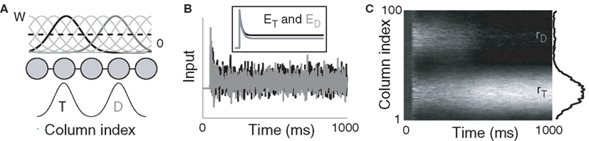
Figure 1. (A) Fully recurrent network simulating 100 cortical columns. Intercolumnar interactions are scaled by down-shifted Gaussian weights W, providing local excitation (support), and distal inhibition (competition) between columns. Gaussian response fields mediate target (T) and distractor (D) input signals. (B) Noisy inputs at the response field centers of the target- (black) and distractor-selective (gray) populations. Inset depicts the mean input. (C) Surface plot of network activity during the decision task. rT and rD refer to firing rates of the target- and distractor-selective populations. Lighter shades correspond to higher-rate activity. The state of the network at the end of the trial is shown on the right side of the figure.
The model is constrained by signature characteristics of neural and behavioral data from visuospatial decision making experiments. The neural data we consider were recorded in LIP, but similar activity is seen in other decision-correlated cortical areas, e.g., the frontal eye fields (see Schall, 2002). These characteristics are (1) decision-correlated neural activity showing an initial “featureless” response (equal magnitude regardless of feature value) followed by a decline in the rate of activity, competitive interactions, and a stereotyped excursion of the “winning” representation (e.g., Dorris and Glimcher, 2004; Sugrue et al., 2004; Ipata et al., 2006; Thomas and Pare, 2007; Churchland et al., 2008); (2) a fixed level of decision-selective activity at the time of the decision (e.g., Roitman and Shadlen, 2002; Churchland et al., 2008); and (3) psychometric and chronometric curves, where accuracy and decision time decrease and increase respectively as a function of task difficulty (see Section 3.1 and Figure 3) and decision times are in the hundreds of milliseconds range (e.g., Roitman and Shadlen, 2002; Palmer et al., 2005; Churchland et al., 2008; Shen et al., 2010). In the context of cortical processing, the first of these characteristics corresponds to a transition from feedforward dominance to feedback dominance, hypothesized to be a fundamental principle of local-circuit cortical processing (see Douglas and Martin, 2007). As we will see, the rate of this transition controls the SAT in our model. The second characteristic provides the motivation for our study, described above. The third characteristic is implicit in the SAT, on the relevant timescale for perceptual decisions.
We simulated a two-choice visual discrimination task by providing two noisy inputs to the model for 1000 ms. The task was to distinguish the stronger input (the target) from the weaker input (the distractor). While the spatial and temporal profiles of the inputs were constrained by the above data, the task clearly generalizes to other decision tasks, just as the model generalizes to other cortical regions. The neural coding of elapsed time (urgency) was simulated with a piecewise linear function (Figure 2C), where the slope of the function was assumed to reflect subjects’ learned estimate of the time available to respond (see Durstewitz, 2004). The activation of each column was simulated with sigmoid function of its input. Gain modulation was implemented by scaling the slope of the sigmoid by the urgency signal during a given trial (Equation 2). As shown in Sections 3.4, 3.5, and 3.6, this approach permits an analysis of the gain-modulated network in trials without gain modulation, where urgency is omitted and the slope of the sigmoid can be set to any value spanned by the scaled slope under gain modulation.
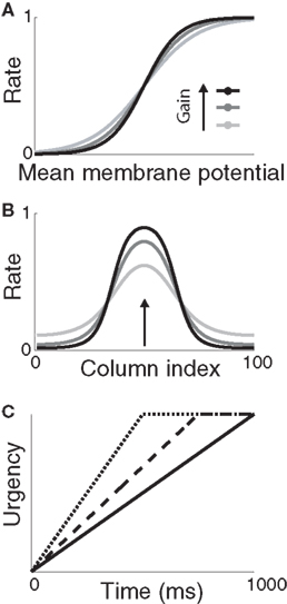
Figure 2. (A) Sigmoid gain function with different values of the slope parameter β. Lighter shades of gray correspond to smaller values of β. (B) Network response (without gain modulation) to a single stimulus for each value of β in (A) above. Curves show network activation at the end of the trial. The simulation was identical to the decision task, but noise was omitted for clarity and only one stimulus was used, centered on column 50 (indicated by the arrow). (C) Urgency signal U(t) building up over 1000 ms (solid), 750 ms (dashed), and 500 ms (dotted). Under gain modulation, β was scaled by U(t) during each trial (see Equation 2, Section 2), akin to a transition from light gray to black in (A,B) with increasing urgency.
We ran 1000 trials across a range of task difficulties and rates of buildup of urgency (Section 2.3). Task difficulty was controlled by the mean similarity of the input signals, ranging from highly distinguishable (90% similar) to indistinguishable (100% similar) on average (Equation 4). Ideal observer analysis of a population of target and distractor-selective columns was used to determine the timing and accuracy of target discrimination on each trial (Section 2.4).
2.1 The Model
The network is a fully connected recurrent rate model with N = 100 nodes, each representing a spatially clustered population of neurons with similar response characteristics (effectively, a cortical column). The firing rate of each population represents the proportion of its neurons emitting a spike at any moment in time (Wilson and Cowan, 1972; Gerstner, 2000). The state of each node i = 1:N (column) is described by
where the phenomenological state variable v is interpreted as the average membrane potential of each neuron in the column (Amari, 1977; Cremers and Herz, 2002), τv = 20 ms is the average membrane time constant, W governs interactions between columns indexed by j = 1:N, s is selective input, described in Section 2.2, and h is normally distributed random noise with mean μh = −10 and SD |μh|, determining the rate to which the network relaxes without selective input, i.e., the resting state (Amari, 1977; Doubrovinski and Herrman, 2009).
The population rate r of each node is related to the state variable v by a sigmoid gain function

where β determines the slope of the function, scaled by urgency signal U(t) as it builds up on each trial. This scaling causes a pivot of the sigmoid around its axis (Figure 2A), but does not shift it to the left or right (Chance et al., 2002). The effect of the scaling on network activation is shown in Figure 2B. In trials with gain modulation, β = 0.0275. In trials without gain modulation (see Section 3.1), U = 0 and we refer to the slope parameter of the sigmoid as  , corresponding to (1 + U(t))·β at any time t under gain modulation.
The intercolumnar interaction structure W is a Gaussian function of the spatial distance between columns arranged in a ring, where excitation-dependent inhibition is provided by subtracting a constant C from this shift-invariant weight matrix (Amari, 1977; Trappenberg and Standage, 2005), depicted in Figure 1A. The strength of interaction between any two columns i and j is thus given by

where d = min(|i − j|Δx, 2π − |i − j|Δx) defines distance in the ring, Δx = 2π/N is a scale factor, and γw = 100 determines the strength of intrinsic (recurrent) activity. Constants σ = 0.75 mm and C = 0.5 support population codes consistent with tuning curves in visual cortex (Mountcastle, 1997; Sompolinsky and Shapley, 1997).
2.2 Simulated Two-Choice Decision Task
To simulate a reaction time version of a two-choice visual discrimination task, Gaussian response fields (RF) were defined for all columns i by  , where d and σ are given above for the intercolumnar interaction structure W. Each column i received selective input
  for time T = 1 s (the stimulus interval). Columns 25 (the target column) and 75 (the distractor column) were maximally responsive to
  and
and  respectively, i.e., the RF centers of the selective inputs were 180° apart in the ring network. Spike response adaptation in upstream visually responsive neurons was modeled by a step-and-decay function (Trappenberg et al., 2001; Wong et al., 2007)
where γs = 75 determines the initial strength of input at the target and distractor columns, μdiv = 3 determines the asymptotic input strength, τμ = 25 ms determines the rate of input decay, and tvrd = 50 ms is a visual response delay (Thomas and Pare, 2007). Constant γμ was set to 1 for the target and to γext for the distractor, where 0.9 ≤ γext ≤ 1 determined target-distractor similarity. The strength of  and
and  respectively was scaled by RFi at each column according to its proximity to the target and distractor columns. In noisy simulations, Gaussian noise with mean and SD μ was added to
  and
and  (Salinas and Abbott, 1996). Our use of the same value of σ for the (extrinsic) RFs and the (intrinsic) lateral interaction structure W is consistent with the feedforward multiplication of accumulators by Gaussian input signals in the multiple-choice decision task of McMillen and Behseta (2010), shown by these authors to be required for asymptotically optimal hypothesis testing. Simulations were run with Euler integration and timestep Δt = 1 ms. A 200-ms equilibration period was used. Mean input to the target and distractor columns is shown in Figure 1B.
2.3 Gain Modulation by the Urgency Signal
The urgency signal was simulated with a piecewise linear function
where Umax = 0.5 and τμ ∈ {500, 750, 1000} ms determines time over which the signal increases toward Umax, depicted in Figure 2C. Gain modulation was implemented by multiplying the slope parameter β = 0.0275 of the columnar gain function by 1 + U(t; Equation 2 above).
2.4 Determining the Timing and Accuracy of Discrimination
Signal detection theory (Green and Swets, 1966) was used to quantify the degree to which an ideal observer of network activation could discriminate the target from the distractor, estimating the separation of the distributions of target and distractor-selective rates at successive 1 ms intervals. Signal detection theory is commonly applied to electrophysiological recordings under conditions in which a target stimulus is inside and (on separate trials) outside a neuron’s response field, averaged over all trials (Thompson et al., 1996; Thomas and Pare, 2007). Because we can observe all the activity in the model, we applied this method to a population of target and distractor-selective columns on each trial. Each population p = 25 included the target and distractor columns plus the adjacent 12 ≈ σ/2πN columns on each side of these response field centers. Receiver operating characteristic curves (ROC) were calculated from the mean rates of these populations, determining mean discrimination for each level of task difficulty and urgency signal U(t). The area under the ROC (AUROC) quantifies the separation of the distributions of target and distractor activation (see Thompson et al., 1996). The probability of discrimination was quantified by a least squares fit of the AUROCs to a cumulative Weibull function

where t is the time after stimulus onset, and a, b, c, and d are fitted parameters: a is the time at which the function reaches 63% of its maximum, b is the slope (shape parameter), and c and d are the upper and lower limits of the function respectively. Parameter c quantifies discrimination magnitude and is typically close to 1 (separate distributions of target and distractor activation at the end of a trial), whereas d is typically close to 0.5 (overlapping distributions at the beginning of a trial, see Figures 4B,C). Because either target or distractor activation could dominate the network on any given trial (correct and error trials respectively), the AUROCs could be fit with increasing or decreasing Weibull functions w. On error trials (decreasing function), a in Equation 6 refers to the time at which w reached 63% of 1 − min(w), and c and d are the lower and upper limits respectively. The time at which w reached 0.75 was considered the discrimination time (Thompson et al., 1996; 0.25 on error trials). The resulting decision times were averaged over all trials to determine the speed of decision making for each task difficulty and urgency U(t). Trials on which w reached neither 0.75 nor 0.25 were considered “no decision” trials.
3 Results
We begin the Section 3 by showing that gain modulation of the network by a growing urgency signal produces the SAT (Section 3.1), where decision-selective activation at decision time is approximately constant across all task conditions, referred to as reaching a fixed threshold (Section 3.2). We subsequently explain these results in terms of the network’s dynamics. Before doing so, it is useful to define some terminology. We define the decision variable as the difference between the activation of the target and distractor columns, and we define the time over which the noise-free model can calculate the decision variable as the network’s effective time constant of integration τeff (Section 3.3). In Section 3.4, we show that as the urgency signal builds up, the network progresses through processing stages supporting a range of integration times, dominated by leakage early in each trial and by feedback inhibition later on (Usher and McClelland, 2001; Bogacz et al., 2006). The latter entails an acceleration of the decision variable, which we refer to as amplification. Note that our use of this term refers to the decision variable only, not to the network processing more generally. In Section 3.5, we show that the within-trial progression from leakage to inhibition-dominated processing allows the network to take advantage of dynamics inherently suited to different stages of the decision process, distinguishing the network from earlier models that produced the SAT with a constant within-trial signal (variable between blocks of trials). In Section 3.6, we take a dynamic systems approach, showing that our numeric explanation corresponds to a bifurcation between dynamic regimes. We analytically calculate the time constant of the linear approximate system, referred to as τlin, which undergoes the same qualitative progression as τeff in Section 3.4. Note that in simulations and analysis without gain modulation, we refer to the network as the fixed-gain network and to the slope parameter of its gain function as  . Thus, for a given value of urgency U(t) in the gain-modulated network,
  in the fixed-gain network. In Section 3.7, we show that the network earns more reward per unit time than a fixed-gain network with
  tuned for best performance.
3.1 Speed and Accuracy of Decisions
For all rates of buildup of urgency U, decisions took longer and became less accurate with increasing task difficulty. The gain-modulated network thus produced typical psychometric and chronometric curves, demonstrating speed, and accuracy of decisions consistent with behavioral data (e.g., Roitman and Shadlen, 2002). Longer buildup of U resulted in slower, more accurate decisions for a given task difficulty (Figure 3). Under the same conditions, shorter buildup resulted in faster, less accurate decisions. The network thus produced the SAT. Of note, with lower task difficulty (90–97% similarity), the network showed another kind of SAT for all U, maintaining near-perfect accuracy by taking longer to make decisions as difficulty was increased, a feature demonstrated by earlier neural models of decision circuits (Wong and Wang, 2006).
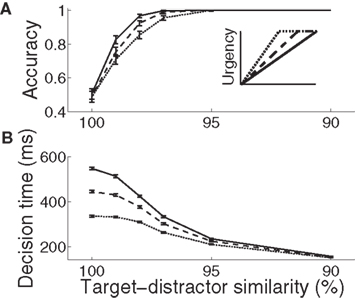
Figure 3. Psychometric (A) and chronometric (B) curves show the SAT in the gain-modulated network. (A) Accuracy: the proportion of trials on which the network correctly discriminated the target. Error bars show 95% confidence intervals. (B) Decision time: mean time of target discrimination (see Section 2). Solid (1000 ms), dashed (750 ms), and dotted (500 ms) curves correspond to the different rates of buildup of U. Error bars show SE. The figure legend corresponds to Figure 2C.
3.2 Target-Selective Activation in the Network
Consistent with neural data (Hanes and Schall, 1996; Churchland et al., 2008), target-selective activation is approximately constant at decision time across all task conditions (between 0.365 and 0.385; Figure 4A). It also reaches a common maximum rate across all conditions (Figures 4B,C), as seen in LIP during visual tasks (Roitman and Shadlen, 2002; Huk and Shadlen, 2005; Churchland et al., 2008). These two findings demonstrate a subtle but important distinction. We used ideal observer analysis to determine stimulus discrimination, so the constant level of activation at decision time demonstrates that a downstream network could employ a fixed threshold when making decisions based on network activity (e.g., the superior colliculus reading out LIP activity). The stereotyped maximum rate of selective activation demonstrates that the network could also employ a fixed threshold to make decisions on its own, i.e., without an observer of its activity. Our results therefore demonstrate that gain modulation by the encoding of urgency can account for the SAT with a fixed threshold, whether a downstream network is reading out the modulated network or if the modulated network has the “final say” on the decision itself. Using a constant threshold to determine speed and accuracy produced similar results to those produced by ideal observer analysis (not shown).
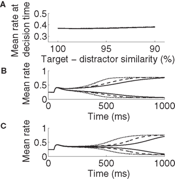
Figure 4. Target-selective activation at decision time is approximately constant (A) and reaches a stereotyped maximum (B,C) across all task difficulties and rates of buildup of U. Solid, dashed, and dotted curves correspond to U building up over 500, 750, and 1000 ms respectively (see Figure 2C). (A) Target-selective rates at discrimination time on correct trials for all task difficulties and buildup of U, determined by ideal observer analysis (see Section 2). (B) Mean activation over the target and distractor populations (25 columns each, see Section 2) on correct trials for 90% target-distractor similarity. The three upper curves show target-selective rates for each U. The three lower curves show distractor-selective rates. (C) Same as in B, but for 99% target-distractor similarity.
3.3 The Effective Time Constant of Integration of the Network
The time over which a recurrent network can accumulate evidence (its effective time constant of integration τeff) can be controlled by parameters determining the strength of network dynamics (Wang, 2002; Wong and Wang, 2006). Above and below an optimal regime, τeff is progressively shortened (Wang, 2008), dominated by amplification and leakage of accumulated evidence respectively (Usher and McClelland, 2001). Larger values of τeff favor accuracy because the network can accumulate evidence for longer. Smaller values favor speed. The ability of the network to trade speed and accuracy as a function of urgency can thus be understood by considering the effect of urgency on its integration time.
We approximated τeff under gain modulation by running a noise-free trial for each U and task difficulty. In each of these trials, we integrated the difference between the firing rates at the target and distractor columns, where τeff was the time at which this difference (the decision variable) stopped growing (precision 10−6). Longer buildup of U yielded longer integration times (Figure 5A). Target-selective rates reached a stereotyped maximum (∼0.85) at τeff for all U and task difficulties. These results are not surprising after the results shown in Figures 3 and 4, but they demonstrate an important principle: slower (faster) buildup of U facilitated longer (shorter) accumulation of evidence under gain modulation, precisely the requirement for the DDM to trade speed and accuracy. We build on this principle below.
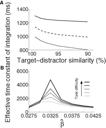
Figure 5. The effective time constant of integration τeff of the network. (A) Solid, dashed, and dotted curves show τeff for urgency buildup over 1000, 750, and 500 ms respectively. Slower buildup yields longer τeff. (B) For all distinguishable tasks (γext < 1) in the fixed-gain network (no gain modulation), τeff increases with  and decreases for
  Shades of gray show that this effect is more pronounced with increasing task difficulty, where lighter shades correspond to easier tasks.
3.4 Urgency Controls the Speed of Transitions Through Processing Stages with Different Effective Time Constants
The above calculation of the network’s effective time constant τeff for each urgency condition explains why the model produces the SAT: slower buildup of U furnishes a longer time constant. But it does not explain how. The mechanism by which gain modulation controls integration time can be understood by measuring τeff in the network without gain modulation (the fixed-gain network) for different values of the slope parameter  Here, the values of τeff can be thought of as successive snapshots of the network’s effective time constant under gain modulation. Consistent with earlier analysis (Wang, 2008), τeff decreased as
  deviated from the value supporting the longest τeff (Figure 5B), that is, above and below this optimal value, the decision variable was increasingly dominated by amplification and leakage respectively.
Under gain modulation, the network progresses through all these processing stages on each trial. As such, the decision variable is dominated by leakage early in the trial when urgency is low and is amplified later in the trial when urgency is high (see Figure 6B). τeff is thus progressively lengthened over the early part of the trial and contracted later on, terminating the decision process. This progression corresponds to a transition from left to right in Figure 5B. In effect, slower buildup of urgency allows the network to spend more time in processing stages with a longer time constant.
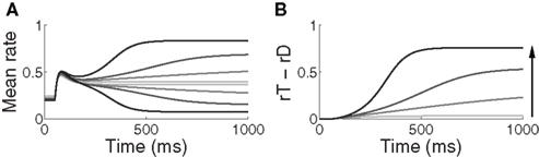
Figure 6. (A) Mean activation over the target- and distractor-selective populations (25 columns each, see Section 2) on a noise-free trial for 97% target-distractor similarity in the fixed-gain network for different values of  Light gray, medium gray, dark gray, and black curves correspond to
  respectively. The four upper curves show target activation. The four lower curves show distractor activation. (B) The difference between the target and distractor activation shown in A. The vertical arrow depicts the transition through processing stages corresponding to each value of (1 + U(t))·β under gain modulation.
Note that our method of calculating τeff is conservative. For example, time constants are often taken at some percentage of the completion of a process, such as half-life. With and without gain modulation (Figures 5A,B respectively), the computed values of τeff are consistent with earlier approximations of cortical network time constants of up to several seconds (Wang, 2002). This would remain the case if τeff was taken at half rise time. Note also that this theoretical construct is not the same thing as decision time, i.e., the decision variable is saturating for much of τeff and a downstream network could read out the decision before saturation.
3.5 A Progression from Leakage to Amplification of the Decision Variable
The progression from leakage to amplification of the decision variable with the buildup of urgency can be further understood by observing the activity in the fixed-gain network during the decision task for different values of  Mean activation over the target and distractor populations on a noise-free trial is shown for one task difficulty (97% similarity) in Figure 6. With low gain, the network distinguishes one signal from the other, but cannot accumulate much of the difference between the signals as the trial progresses (Figure 6B, lightest gray curves). As such, the network is capable of functioning as a noise filter, recognizing a difference between input signals, but leakage and inhibition are soon balanced (Usher and McClelland, 2001). With increased gain, the network integrates the difference between signals over the full trial, approximating the DDM, as evidenced by the near-linear increase of the decision variable (medium gray). With a further increase in gain, the network amplifies an integrated difference between inputs (dark gray). With high gain, the network quickly amplifies a small difference, demonstrating dynamics suitable for categorical choice (black). The precise correspondence between the slope parameter
  of the gain function and each of these stages depends on the mean difference between signals, but other task difficulties yield similar curves.
Whereas the fixed-gain network implements a single regime for each value of  the gain-modulated network transitions through these regimes on each trial, where the rate of transition is determined by the timecourse of the urgency signal U. Thus, with gain modulation, the network smoothly progresses through a series of processing stages implementing noise filtering, difference integration, difference amplification, and selection. As such, the network begins each trial conservatively (dominated by leakage), but becomes less so as information is accumulated. The slower the buildup of U, the longer the network spends in more conservative stages, enabling higher accuracy at the expense of speed. This progression is depicted by the vertical arrow in Figure 6B. The outcome of the different rates of progression can be seen in the mean target and distractor-selective activation under gain modulation shown in Figures 4A,B, where activation diverges more slowly with slower buildup of U. Figure 3 shows the resulting SAT.
3.6 Non-Linear Dynamic Analysis of the Model
The above simulations demonstrate the SAT with a fixed neural threshold and provide an intuitive picture of network dynamics with growing urgency. In this section, we take a non-linear dynamics approach to formally characterize this picture.
3.6.1 Two regimes for decision making
From a dynamic systems point of view, the accumulation of evidence in the network is the evolution of a dynamic system from an initial state to an attractor corresponding to the target or the distractor. The evolution is determined by the structure of the steady states of the system (Strogatz, 2001). In our model, the slope parameter β, urgency signal U, and the target-distractor similarity γext determine the steady states of the system defined by Equation 1. By setting the right hand side of Equation 1 to zero, we obtain a set of algebraic equations, the solution of which gives the steady states. Based on the steady state of the system, the decision process can be classified according to two regimes: in regime 1, the system evolves directly from the initial state to a single attractive stable steady state (see Figure 7A). In regime 2, the system is driven away from one unstable steady state to one of two stable steady states (see Figure 7B).
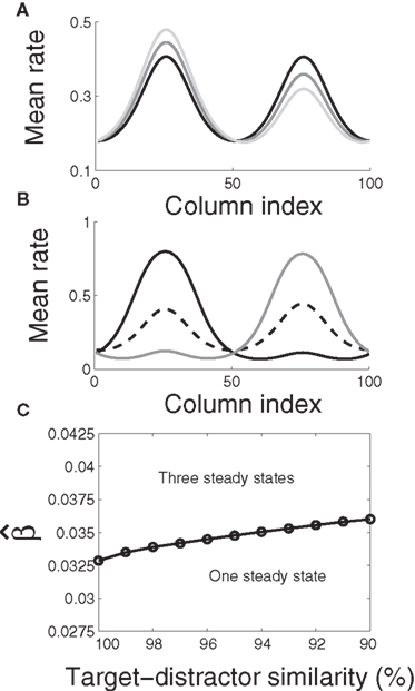
Figure 7. The steady states of the system. (A) The system (Equation 1) has one steady state, which is stable. For U = 0 and target-distractor similarity γext ∈ {1.0, 0.95, 0.9}, the stable steady state has two bumps, corresponding to the target and the distractor. In the indistinguishable case (γext = 1), the stable steady state is symmetric. Otherwise, the height of the target bump is higher than the distractor bump. (B) The system has three steady states. Black and gray solid lines correspond to the stable steady states and the dashed line corresponds to the unstable steady state (U = 0.4 and γext = 0.97). The height of the larger bump in each of the two stable steady states is almost equal and changes slightly with γext. The difference in height of the two bumps in the unstable steady state increases with decreasing γext. (C) The bifurcation diagram of the system. The parameter domain is separated into two regions: a region with one steady state and a region with three steady states.
The two regimes have several notable features. Firstly, the similarity of the target and the distractor plays a different role in each regime. In regime 1, the height of the bump related to the target is higher than the bump related to the distractor for distinguishable tasks (γext < 1, see Figure 7A). The difference between the two bumps decreases with increasing target-distractor similarity γext. In regime 2, one stable steady state has a higher bump corresponding to the target and a lower bump corresponding to the distractor; the other stable steady state has a higher bump corresponding to the distractor and a lower bump corresponding to the target. The unstable steady state has two comparable bumps, where the higher bump corresponds to the distractor and the lower bump corresponds to the target (see Figure 7B). The difference between the two bumps in the unstable steady state also decreases with increasing target-distractor similarity.
Secondly, by variation of the target-distractor similarity γext and the urgency signal U (or the slope parameter β), we obtain the bifurcation diagram of the system. As shown in Figure 7C, there are two regions in the plane of (1 + U)·β over γext. The system has one stable steady state in one region and three steady states in the other.
Thirdly, the evolution from the initial state to the stable steady state is determined by the structure of the steady states. In regime 1, the system evolves directly from the initial state to the single stable steady state of the target. The dynamics in the vicinity of this stable state determine the characteristics of the decision. In regime 2, the initial firing rate of the target population equals that of the distractor population (see Figure 4), so the initial state is in the vicinity of the two-bump unstable steady state. Therefore, the evolution from the initial state to the stable steady state is determined by the dynamics in the vicinity of the unstable steady state.
3.6.2 Regimes for accuracy and decisiveness
As described above, the decision ensues with the evolution of the system to the stable steady state. The dynamics in the vicinity of the steady state (the stable steady state in regime 1 and the unstable steady state in regime 2) thus determine task performance, such as speed, accuracy, and decisiveness (whether or not a decision is made). We have used signal detection theory to determine the decision on each trial, where the AUROC is used to estimate the separation of the distributions of target and distractor-selective activation. On any given trial, the activation of the noisy system fluctuates around the rates of the noise-free system. Therefore, the overlap of the two distributions decreases (and thus the AUROC increases) with the increase of the difference between the target and distractor-selective activation in the noise-free system. In regime 1, if the difference between the two bumps of the stable steady state is small [i.e., a low value of (1 + U)·β and a high value of γext], the two distributions overlap too much to be discriminated and the network cannot make a decision. However, if the difference between the two bumps of the stable steady state is large enough to be discriminated, the network cannot make errors.
In regime 2, the system is driven away from the unstable steady state to one of the two stable steady states, where the difference between target and distractor-selective activation is large enough to make a decision (see  in Figure 6). Because the system is sensitive in the vicinity of the unstable steady state, it may be driven in the wrong direction by noise, i.e., it can make errors in regime 2. Thus, the network is decisive, but makes some mistakes in regime 2, whereas it either makes correct decisions or no decision at all in regime 1.
3.6.3 The time constant of the approximate linear system
In the vicinity of the steady state, the dynamic system (Equation 1) can be linearized as

where  is interpreted as the mean membrane potential,
  is the steady state of the system,
  is the ith eigenvector, λi is the ith eigenvalue, and ci is the projection of the difference between the initial state and the steady state, defined by
In regime 1, the eigenvalues for the stable steady state are negative, and the evolution of the system along the invariant manifold tangent to the eigenvector corresponding to the largest eigenvalue (i.e., the one closest to 0) determines how slowly the system reaches the stable steady state. Therefore, the absolute value of the reciprocal of the largest eigenvalue can be used to approximate the time it takes for the system to reach the stable steady state and is defined as the time constant. In regime 2, we consider the time it takes for the system to evolve away from the unstable steady state. The reciprocal of the largest positive eigenvalue approximates the time over which the system departs from the unstable steady state of the invariant manifold tangent to the eigenvector corresponding to the largest eigenvalue. Therefore, the absolute reciprocal of the largest eigenvalue of the stable steady state in regime 1 and the unstable steady state in regime 2 depicts the time over which the system makes a decision and is denoted τlin.
For a given target-distractor similarity γext, the system operates in regime 1 or regime 2, depending on the value of  (Figure 7). The time constant τlin is shown for three values of γext in Figure 8, where for each curve, the left side of the discontinuity shows the time constant of the stable steady state in regime 1, and the right side shows the time constant of the unstable steady state in regime 2. These curves show the same qualitative increase and subsequent decrease with increasing of
  shown for integration times in Figure 5B, where more difficult tasks have longer time constants. The slight exceptions to these characteristics occur in the vicinity of the bifurcation, where the time constant is undefined because the eigenvector is zero at the bifurcation point, but the progression through processing stages with different time constants described in Sections 3.3 and 3.5 is clear. Notably, the time constants in Figures 5 and 8 peak at approximately the same value of
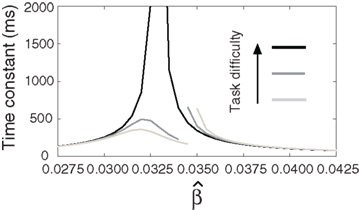
Figure 8. The time constant of the steady state τlin. For each target-distractor similarity γext, the network operates in regime 1 with low (1 + U)·β and subsequently in regime 2 with high (1 + U)·β. Thus, the left side of each curve shows the time constant for the stable steady state of regime 1, and the right side shows the time constant for the unstable steady state of regime 2. For γext = 1, the time constant increases in regime 1 and decreases in regime 2. For γext = 0.97 and 0.95, the time constant increases and then decreases in regime 1, peaking at approximately  , consistent with the simulations in Figure 5. The time constant decreases in regime 2 for all γext.
3.6.4 The dynamics of decision making with growing urgency
With growing urgency, decision processing under gain modulation can be described according to the above two regimes. In the early stages of a decision, the system operates in regime 1 because the urgency signal is low. The system has only one stable steady state with activation bumps centered at the target and distractor columns. As the urgency signal grows, the target and distractor-selective activation in the steady state gradually increases and decreases respectively (see Figures 9A–C). This changing stable steady state is tracked by the system and consequently the target and distractor-selective activation in the network gradually increases and decreases respectively before the urgency signal exceeds the bifurcation threshold (Figure 7C). If the urgency signal does not cross the bifurcation threshold, the system will approach the stable steady state of the final urgency signal. If the difference between the target and distractor-selective activation is large enough, the system makes a correct decision, otherwise, it makes no decision. Once the urgency signal exceeds the bifurcation threshold, the system operates in regime 2 and the stable steady state splits into three steady states, one unstable and two stable (see Figures 9D–F). At the same time, the state of the system, which tracks the stable steady state in regime 1 and whose target-selective activation is stronger than the distractor-selective activation, falls into the vicinity of the unstable steady state in regime 2. Driven away from the unstable steady state, the system evolves to one of the stable steady states (corresponding to the target or the distractor) and makes a decision.
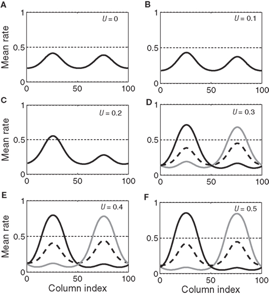
Figure 9. The evolving steady states of the network with growing urgency. As urgency U(t) builds up on each trial, the network undergoes a bifurcation from a regime with a single stable steady state (A–C, regime 1 in the text) to a regime with one unstable steady state and two stable steady states (D–F, regime 2 in the text). In the latter, one stable steady state corresponds to the target (solid black) and one to the distractor (gray). Target-distractor similarity in the figure was γext = 0.97. The dotted horizontal line (A–F) helps to gage the size of the bumps and has no other significance.
In the fixed-gain network, the decision process occurs either in regime 1 or in regime 2, depending on the slope parameter  and the target-distractor similarity γext. For distinguishable tasks under gain modulation, if the urgency signal is big enough to cross the bifurcation threshold (0.95 < γext < 1), the progression from regime 1 to regime 2 allows the network to begin regime 2 in a state closer to the target attractor than would be the case in the fixed-gain network with slope parameter
  equal to
  where
where  is the time at which U crosses the bifurcation threshold. This advantageous position of the network state formally characterizes the progression described in Section 3.5, where early noise filtering allows late amplification of a high-quality decision variable. As described in Section 3.6.3, the progression stretches the time constant τlin as the system moves through regime 1, before contracting it in regime 2 on the way to the stable steady state of the target or the distractor. Speed and accuracy are traded because the time constant τlin and the decision variable are larger at decision time with slower buildup of U (not shown). When the decision occurs in regime 1, the decision variable is larger at decision time with faster buildup of U, but accuracy is not compromised because the network cannot make errors.
3.7 Optimal Decision Making
The above analysis shows that the bifurcation between regime 1 and regime 2 under gain modulation puts the network in a state closer to the target attractor when it enters regime 2 than would be the case in the fixed-gain network with slope parameter  equal to
  at the time of the bifurcation
  . This analysis suggests that gain modulation by the urgency signal may produce more accurate decisions per unit time than the fixed-gain network. To investigate this possibility, we calculated the reward rate over a full block of 6000 trials (1000 trials for six values of target-distractor similarity γext) under gain modulation for each of the above rates of buildup of U. Because the urgency signal simulates an estimate of the time available to respond (see Durstewitz, 2004), τu = 1000 ms corresponds to an accurate estimate of the deadline and τu < 1000 ms corresponds to an underestimate. We also considered an overestimate of τu, running a full block of trials for τu = 1250 ms, where the trial time was still 1000 ms, i.e., U(t) never reaches Umax. We also ran a full block of trials with the fixed-gain network for a range of values of
  including several values near the best-performing
  to ensure we were not missing a finely tuned optimum (see Figure 10).
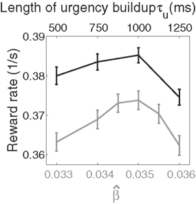
Figure 10. Reward rate over a full block of trials as a function of the buildup of urgency under gain modulation (black) and the slope parameter of the gain function  in the fixed-gain network (gray). The time over which the urgency signal U(t) builds up corresponds to an underestimate (τu ∈ {500, 750} ms), an accurate estimate (τu = 1000 ms) and an overestimate (τu = 1250 ms) of the trial deadline. Error bars show SE.
Because mean decision time on error trials was longer than on correct trials under gain modulation (see Section 4.3), we followed the reward rate definition of Eckhoff et al. (2009), where penalties on error trials were considered implicit in decision time. Reward rate was thus defined on each trial as R = A/(DT + NDL), where A is accuracy (one for correct decisions and zero for errors or no decision trials), DT is decision time, and NDL is non-decision latency. NDL subsumed the post-decision motor response (≈200 ms), an interval between trials (≈1750 ms), and the visual response delay (50 ms, see Section 2). Non-decision latency was thus 2000 − 50 = 1950 ms. As shown in Figure 10, reward rates were systematically higher in the gain-modulated network and were maximal when U(t) peaked at the trial deadline, i.e., of the urgency signals tried, an accurate estimate of the trial length was optimal in terms of maximizing reward (Figure 10). These findings were qualitatively reproduced with the reward rate definition of Gold and Shadlen (2002; not shown).
This finding is instructive in several regards. Earlier work showed that a spatially non-selective signal, variable between blocks of trials, but constant within each trial, could potentially produce the SAT with a fixed threshold (Bogacz et al., 2006; Furman and Wang, 2008). This approach is equivalent to setting U to a fixed value between trials in our model and could be instantiated by goal-directed persistent activity in higher association cortical areas (see Goldman-Rakic, 1995; Wang, 2001). This mechanism is plausible, though we are unaware of any data showing the rate of persistent activity to vary systematically between trials or blocks of trials, as would be required. There is a growing body of data showing the neural encoding of elapsed time relative to learned intervals (see Durstewitz, 2004), previously correlated with decisions (Churchland et al., 2008) and proposed here to control the SAT. The analysis in Section 3.6 and the calculation of reward rate in this section show that a within-trial signal is optimal in our model, though we expect within-trial and between-trial gain modulation to play complimentary roles in decision making and cognitive function more generally (see Section 4.4).
4 Discussion
Our model offers a candidate neural mechanism for the SAT. We propose that gain modulation by the encoding of urgency controls the time constant of cortical decision circuits “on the fly.” The rate of buildup of urgency determines how long the circuit integrates evidence before the decision variable is amplified. Longer (shorter) estimates of the time available to respond result in slower (faster) buildup of the signal, so the circuit spends more (less) time integrating evidence. Importantly, decision-correlated neural activation reaches a fixed level at decision time, consistent with neural data (see Schall, 2001). In effect, the encoding of urgency determines the rate of growth of the decision variable, instantiated by the well established mechanisms of gain modulation (Salinas and Thier, 2000; Salinas and Sejnowski, 2001) and the encoding of the passage of time (Durstewitz, 2004; Mauk and Buonomano, 2004; Buhusi and Meck, 2005).
4.1 A Neural Mechanism for Time-Variant Drift Diffusion with a Fixed Threshold
Our neural model is grounded in abstract, mathematical models that have been instrumental in characterizing decision processes. Sequential sampling models are based on the premise that evidence is integrated until it reaches a threshold level (see Smith and Ratcliff, 2004). Because evidence may be incomplete or ambiguous and neural processing is noisy, temporal integration provides an average of the evidence, preventing decisions from being made on the basis of momentary fluctuations in either the evidence or processing. The longer the integration time, the better the average (see Bogacz, 2007). In two-choice tasks, integrating the difference between the evidence favoring each option implements the DDM, known to yield the fastest decisions for a given level of accuracy and the most accurate decisions for a given decision time (see Bogacz et al., 2006). The DDM thus optimizes speed and accuracy for a given threshold. The SAT can be achieved by varying the threshold, a principle suggested to be instantiated in the brain (Gold and Shadlen, 2002).
The DDM has been augmented with a time-variant mechanism similar in principle to our use of urgency (differences between the models are described below). In the model by Ditterich (2006b), the decision threshold is lowered over the course of each trial. This approach is functionally equivalent to an increasing multiplication of the evidence as the trial progresses, demonstrated to earn more reward per unit time than the standard DDM in a two-choice task with no explicit deadline (Ditterich, 2006a). The time-dependent multiplication of evidence permits the effect of urgency with a fixed threshold, so this abstract model is consistent with neural data in that regard. Although the SAT was not a focus of these studies, varying the rate of either time-dependent mechanism would effectively trade speed and accuracy.
Neural models have addressed the possible mechanisms underlying the above mathematical models, several of which have been shown to be equivalent to the DDM under biophysical constraints. In these models, the subtractive operation is implemented by mutual inhibition between neural populations selective for each option of a decision (Bogacz et al., 2006), a ubiquitous neural process that scales naturally with the number of options (Usher and McClelland, 2001). Recurrent processing allows slow integration, where network dynamics yield effective time constants much longer than those of contributing biophysical processes (e.g., the time constants of synaptic receptors; Wang, 2002). This neural framework accounts for wealth of neural and behavioral data (see Schall, 2001; Gold and Shadlen, 2007; Wang, 2008). Varying a threshold firing rate will trade speed and accuracy in these models, but, as described above, it conflicts with experimental data (see Schall, 2001).
Our model trades speed and accuracy with a fixed threshold by exploiting the time constant of recurrent networks (Sections 3.3 and 3.6.3). Previous work showed that biophysically based parameters determine an optimal processing regime (Wang, 2002; Wong and Wang, 2006), above and below which the time constant is monotonically shortened (Wang, 2008), dominated by inhibition and leakage respectively (Usher and McClelland, 2001; Bogacz et al., 2006). In these studies, networks were tuned to a single set of parameters that were chosen for best performance. This configuration was then used in a decision task. Unlike these models, our network employs a range of time constants on each trial, where speed and accuracy are traded according to the rate of progression from leakage to inhibition-dominated processing (Sections 3.4 and 3.5). The rate of progression is determined by the urgency signal. Because the network passes through the same processing stages in all cases, its activity follows the same trajectory and decisions can be made with a fixed threshold. In effect, faster (slower) buildup of urgency contracts (expands) the progression in time, but nothing else changes.
4.2 Biological Correlates of the Model
We have used a network belonging to a class of local-circuit models (Wilson and Cowan, 1973; Amari, 1977) widely used to simulate cortical processing of continuous feature values such as spatial location (Camperi and Wang, 1998; Standage et al., 2005). These models are referred to by a number of names, including dynamic neural fields (Trappenberg, 2008), line attractor networks (Furman and Wang, 2008) and basis function networks (Pouget et al., 2000). The model’s foundations are based on a columnar structure where inhibition is broadly tuned and the probability of lateral excitatory synaptic contact is normally distributed (see White, 1989; Abeles, 1991; Goldman-Rakic, 1995).
We have modeled subjects’ estimates of the passage of time with a piecewise linear function, where different slopes correspond to different urgency conditions (Figure 2C). While this first approximation is clearly simplistic, it is supported by neural data showing approximately linear ramping that reaches a common peak around the time of an anticipated event (see Durstewitz, 2004). In reaction time tasks with a deadline (Schall and Hanes, 1993; McPeek and Keller, 2004; Thomas and Pare, 2007), such activity would provide an explicit encoding of the urgency to respond. Even in reaction time tasks without a deadline, it is common to constrain the timing of reward to discourage fast reaction times (Roitman and Shadlen, 2002; Huk and Shadlen, 2005), motivating subjects to self-impose deadlines that limit the time between trials (and thus rewards). Neural correlates of temporal estimates have been described in posterior parietal cortex (Leon and Shadlen, 2003; Janssen and Shadlen, 2005), prefrontal cortex (Genovesio et al., 2006), premotor cortex (Mita et al., 2009), and the mid-brain superior colliculus (Thevarajah et al., 2009) among other structures. These data suggest that temporal coding mechanisms can be more complex than linear ramping activity, but the model is by no means limited to the linear case. For example, in the DDM with a collapsing threshold, best performance was achieved with a logistic function of time, rather than a linear function (Ditterich, 2006b). Whether and how different urgency signals affect the model is left to a follow up study.
Neural mechanisms that may underlie gain modulation include recurrent processing of spatially non-selective input (Salinas and Abbott, 1996), voltage-dependent dendritic non-linearities (Mel, 1993; Larkum et al., 2004), and changes in cellular input–output relationships caused by temporal correlations in input activity (Salinas and Sejnowski, 2001), background noise (Chance et al., 2002; Prescott and Koninck, 2003; Higgs et al., 2006), and other factors leading to variable conductance states (Destexhe et al., 2003). Our method of gain modulation was meant to abstract over such mechanisms. Note that alternative methods of gain modulation lead to similar results, including the multiplication of network activity by the urgency signal, and the urgency-dependent increase in the strength of recurrent connections (not shown).
4.3 Differences with Earlier Time-Variant Models of Decision Making
While conceptually similar to Ditterich’s (2006a) time-variant DDM, our network model differs in a crucial respect: the evolving decision variable is subject to gain modulation, not just the instantaneous evidence. Consider the DDM performing a two-choice decision task. As above, let st and sd refer to noisy evidence for the target and distractor respectively. At any instant, the difference between the evidence for each option is x(t) = st(t) − sd(t), which is integrated over time. Let X refer to the running total (the decision variable). The time at which the absolute value |X| exceeds a threshold υ > 0 is the decision time. If X is positive at the decision time, the target is chosen. If X is negative, the distractor is chosen. We may therefore express the DDM as
In the time-variant DDM (Ditterich, 2006a), st and sd are multiplied by an increasing temporal signal similar to the urgency signal U. Thus, Ditterich’s model may be expressed as
Like Equation 10, the input signals to our network model are subject to an increase in gain, but so is the recurrent processing of the decision variable. The subtractive operation is supported by recurrent inhibition. We may thus express our model as

where α is a (positive) scale factor. The practical difference between the two models is the time of arrival of the evidence subject to strong amplification. In Equation 10 (and in Ditterich’s model), an increasing urgency signal gives greater weight to later evidence than earlier evidence because only the input is amplified. In Equation 11 (and in our network model), there is a transition from a heavier weighting of the input to a heavier weighting of the decision variable, similar to the transition from extrinsic to intrinsic processing hypothesized to be a fundamental principle of local-circuit cortical processing (see Douglas and Martin, 2007). The urgency signal governs the rate of this transition.
The implications of the difference between the two models can be seen in Figure 11A for a noisy trial with 99% target-distractor similarity, where Equations 10 and 11 were given the same inputs received by the target and distractor columns in the network, Umax = 10 (Equation 5) and α = 1/1000. Equation 11 makes different decisions for different rates of urgency buildup. With faster buildup, the model effectively ignores later evidence (see figure caption). In contrast, Equation 10 is always dominated by its inputs. This feedforward dominance is clearly shown in Figures 11B,C, where the evidence for the target and the distractor was switched in the fourth and first quartiles of a noise-free trial respectively (see figure caption). An attractive feature of Equation 11 is the explosion of the decision variable (black curves in the figure), alleviating the need for fine tuning of the decision threshold, similar in principle to the subcritical bifurcation in the non-linear diffusion model by Roxin and Ledberg (2008).
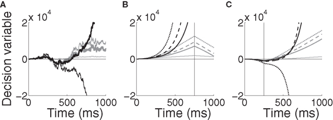
Figure 11. Time-variant DDMs given by Equations 10 (dark gray, modulation of the inputs) and 11 (black, modulation of the inputs and the decision variable). (A) A noisy trial with mean target-distractor similarity 99%. The DDMs received the same inputs as the target and distractor columns in the network with urgency building up over 1000 ms (thick curves) and 500 ms (thin curves). The inputs to each model were identical, including noise. The light gray curve shows the standard DDM (Equation 9, no urgency). Parameters are given in the text. (B) Noise-free trial with changing evidence for target-distractor similarity 90% and urgency buildup over 1000 ms (solid), 750 ms (dashed) and 500 ms (dotted). The vertical line indicates the switching of the target and distractor stimuli over the last quarter of the trial. Step inputs were used (no decay) and the visual response delay was omitted. The light grey curve shows the standard DDM (Equation 9, no urgency). (C) Same as in (B), but the evidence was switched during the first quarter and in Equation 11 was increased from 1/1000 to 1/750.
While the difference between these time-variant DDMs is clear from Equations 10 and 11 and Figure 11, we do not further investigate the novel DDM introduced by Equation 11 in this paper. Suffice to say, we anticipate that Equations 10 and 11 will produce similar results over a block of trials with constant mean evidence (within each trial), the dominant experimental approach to date (e.g., Roitman and Shadlen, 2002; Thomas and Pare, 2007; Churchland et al., 2008). However, in trials with interference stimuli (Huk and Shadlen, 2005) or changing evidence (Cisek et al., 2009), results will differ due to the timing of amplification. It is worth noting that both models produce error trials that are longer than correct trials, but they do so for different reasons. As elegantly explained by Ditterich (2006b), error trials are longer than correct trials in his model because noise grows faster than drift rate; the lower signal-to-noise ratio later in trials leads to more errors, so error trials are longer on average. Here, error trials take longer because the system has to cross the invariant manifold of the unstable steady state, which takes more time.
Our model also bears conceptual similarities with the “urgency gating” models of Cisek et al. (2009). In their study, mathematical models were compared for their ability to explain data from decision tasks with changing evidence. Under noisy conditions, the most successful model multiplied elapsed time by a low-pass filter of the evidence, which can be thought of as a brief spatiotemporal average. Notably, their data suggest that urgency controls the SAT. Our model provides a neural mechanism by which such control may be exerted.
4.4 Flexible Modulation of Decision Circuitry on More than One Timescale
Ultimately, the modulation of decision circuitry is likely to occur on more than one timescale. Two such timescales are captured by the mathematical models of Gold and Shadlen (2002) and Ditterich (2006b). The former specifies a decision threshold for the DDM for all trials of an experiment (or some set of decisions). The latter adjusts the decision threshold on a within-trial basis, lowering it over the course of each trial. Although our neural model uses a within-trial approach, it offers a time-variant mechanism that in principle, can flexibly implement either or both approaches. The gain-modulated network began and ended each trial in extreme regimes dominated by leakage and inhibition respectively. These rough parameters account for the SAT, but modulation of cortical processing occurs on longer timescales as well, providing a mechanism for instantiating the approach of Gold and Shadlen (2002). Trial-to-trial modulation could be implemented in our model by varying the initial strength of the network on each trial (the initial value of β) depending on previous choices and their reward outcomes (Dorris et al., 2000; Thevarajah et al., 2010). Within-trial and between-trial modulation are both potentially supported by the different timescales of dopamine signals (see Schultz, 2007). Dopamine is extensively correlated with reward (see Schultz, 2006) and can modulate gain in cortical circuitry (see Seamans and Yang, 2004). We thus envision trial-to-trial and within-trial modulation playing complementary roles in decision making.
4.5 Summary and Conclusions
Models of decision circuits have demonstrated that network dynamics determine time constants of integration (Wang, 2002, 2008; Wong and Wang, 2006) and that corresponding processing regimes are subject to modulation (Eckhoff et al., 2009). To date, however, neural models instantiating the DDM have used a single mechanism to control speed and accuracy: the difference between the decision threshold and the level of activity on which the decision variable builds (see Bogacz et al., 2006 for analysis of these models). If sufficiently variable, initial levels of activity could account for the SAT with a constant threshold. Here, we propose another, compatible mechanism. In the context of sequential sampling models, the crucial factor is integration time, control of which is not limited to the difference between initial and threshold levels of activity. In this regard, it is instructive to distinguish between the quality of the decision variable and the rate of neural activation sufficient for the decision. For example, network dynamics force decisions in our model when the target and distractor are identical on average, also shown by earlier models (Wang, 2002; Wong and Wang, 2006). This property is useful because decisions often have deadlines, but the quality of the decision variable is low in these cases.
The notion of urgency in decision making is not new (Reddi and Carpenter, 2000) and is an instance of the concept of hazard rate, or the anticipation of an upcoming event (Luce, 1986; Janssen and Shadlen, 2005). A growing body of experimental data suggests that the encoding of time is as natural a process as the encoding of space (see Durstewitz, 2004; Mauk and Buonomano, 2004; Buhusi and Meck, 2005). When faced with deadlines, either self-imposed or imposed by the environment, it appears we automatically encode the urgency to respond. At least one empirical study has quantified the representation of urgency along these lines, where neural activity was correlated with both the passage of time and subjects’ decisions in a decision task, independent of the evidence (Churchland et al., 2008). Our study proposes a neural mechanism by which integration and urgency are combined: decisions are based on integrated evidence, but integration time is controlled by the representation of urgency.
Conflict of Interest Statement
The authors declare that the research was conducted in the absence of any commercial or financial relationships that could be construed as a potential conflict of interest.
Acknowledgments
This work was supported by the Canadian Institutes of Health Research. Da-Hui Wang was supported by NSFC under Grant 60974075. Dominic Standage thanks Martin Paré and Thomas Trappenberg for helpful discussions.
References
Abeles, M. (1991). Corticonics: Neural Circuits of the Cerebral Cortex. Cambridge: Cambridge University Press.
Amari, S. (1977). Dynamics of pattern formation in lateral-inhibition type neural fields. Biol. Cybern. 27, 77–87.
Andersen, R. A., Essick, G. K., and Siegel, R. M. (1985). Encoding of spatial location by posterior parietal neurons. Science 230, 456–458.
Andersen, R. A., and Mountcastle, V. B. (1983). The influence of the angle of gaze upon the excitability of the light-sensitive neurons of the posterior parietal cortex. J. Neurosci. 3, 532–548.
Ben-Yishai, R., Bar-Or, R. L., and Sompolinsky, H. (1995). Theory of orientation tuning in visual cortex. Proc. Natl. Acad. Sci. U.S.A. 92, 3844–3848.
Bogacz, R. (2007). Optimal decision-making theories: linking neurobiology with behaviour. Trends Cogn. Sci. 11, 118–125.
Bogacz, R., Brown, E., Moehlis, J., Holmes, P., and Cohen, J. D. (2006). The physics of optimal decision making: a formal analysis of models of performance in two-alternative forced-choice tasks. Psychol. Rev. 113, 700–765.
Buhusi, C. V., and Meck, W. H. (2005). What makes us tick? Functional and neural mechanisms of interval timing. Nat. Rev. Neurosci. 6, 755–765.
Camperi, M., and Wang, X.-J. (1998). A model of visuospatial working memory in prefrontal cortex: recurrent network and cellular bistability. J. Comput. Neurosci. 5, 383–405.
Chance, F. S., Abbott, L., and Reyes, A. D. (2002). Gain modulation from background synaptic input. Neuron 35, 773–782.
Churchland, A. K., Kiani, R., and Shadlen, M. N. (2008). Decision-making with multiple alternatives. Nat. Neurosci. 11, 693–702.
Cisek, P. (2006). Integrated neural processes for defining potential actions and deciding between them: a computational model. J. Neurosci. 26, 9761–9770.
Cisek, P., Puskas, G. A., and El-Murr, S. (2009). Decisions in changing conditions: the urgency-gating model. J. Neurosci. 29, 11560–11571.
Cremers, D., and Herz, A. V. M. (2002). Traveling waves of excitation in neural field models: equivalence of rate descriptions and integrate-and-fire dynamics. Neural. Comput. 14, 1651–1667.
Destexhe, A., Rudolph, M., and Paré, D. (2003). The high-conductance state of neocortical neurons in vivo. Nat. Rev. Neurosci. 4, 739–751.
Ditterich, J. (2006b). Stochastic models of decisions about motion direction: behavior and physiology. Neural Netw. 19, 981–1012.
Dorris, M. C., and Glimcher, P. W. (2004). Activity in posterior parietal cortex is correlated with the relative subjective desirability of action. Neuron 44, 365–378.
Dorris, M. C., Pare, M., and Munoz, D. P. (2000). Immediate neural plasticity shapes motor performance. J. Neurosci. 20, 1–5.
Doubrovinski, K., and Herrman, J. M. (2009). Stability of localized patterns in neural fields. Neural. Comput. 21, 1125–1144.
Douglas, R. J., and Martin, K. A. C. (2007). Recurrent neuronal circuits in the neocortex. Curr. Biol. 17, R496–R500.
Eckhoff, P., Wong-Lin, K. F., and Holmes, P. (2009). Optimality and robustness of a biophysical decision-making model under norepinephrine modulation. J. Neurosci. 29, 4301–4311.
Furman, M., and Wang, X.-J. (2008). Similarity effect and optimal control of multiple-choice decision making. Neuron 60, 1153–1168.
Genovesio, A., Tsujimoto, S., and Wise, S. P. (2006). Neuronal activity related to elapsed time in prefrontal cortex. J. Neurophysiol. 95, 3281–3285.
Gerstner, W. (2000). Population dynamics of spiking neurons: fast transients, asynchronous states, and locking. Neural. Comput. 12, 43–89.
Gold, J. I., and Shadlen, M. N. (2001). Neural computations that underlie decisions about sensory stimuli. Trends Cogn. Neurosci. 5, 10–16.
Gold, J. I., and Shadlen, M. N. (2002). Banburismus and the brain: decoding the relationship between sensory stimuli, decisions, and reward. Neuron 36, 299–308.
Gold, J. I., and Shadlen, M. N. (2007). The neural basis of decision making. Annu. Rev. Neurosci. 30, 535–574.
Hanes, D. P., and Schall, J. D. (1996). Neural control of voluntary movement initiation. Science 274, 427–430.
Higgs, M. H., Slee, S. J., and Spain, W. J. (2006). Diversity of gain modulation by noise in neocortical neurons: regulation by the slow afterhyperpolarization conductance. J. Neurosci. 26, 8787–8799.
Huk, A. C., and Shadlen, M. N. (2005). Neural activity in macaque parietal cortex reflects temporal integration of visual motion signals during perceptual decision making. J. Neurosci. 25, 10420–10436.
Ipata, A. E., Gee, A. L., Gottlieb, J., Bisley, J. W., and Goldberg, M. E. (2006). LIP responses to a popout stimulus are reduced if it is overtly ignored. Nat. Neurosci. 9, 1071–1076.
Janssen, P., and Shadlen, M. N. (2005). A representation of the hazard rate of elapsed time in macaque area LIP. Nat. Neurosci. 8, 234–241.
Larkum, M. E., Senn, W., and Luscher, H.-R. (2004). Top-down dendritic input increases the gain of layer 5 pyramidal neurons. Cereb. Cortex 14, 1059–1070.
Leon, M. I., and Shadlen, M. N. (2003). Representation of time by neurons in the posterior parietal cortex of the macaque. Neuron 38, 317–327.
Luce, R. D. (1986). Response Times: Their Role in Inferring Elementary Mental Organization. New York: Oxford University Press.
Mauk, M. D., and Buonomano, D. V. (2004). The neural basis of temporal processing. Annu. Rev. Neurosci. 27, 307–340.
McMillen, T., and Behseta, S. (2010). On the effects of signal acuity in a multi-alternative model of decisionmaking. Neural. Comput. 22, 539–580.
McPeek, R. M., and Keller, E. L. (2004). Deficits in saccade target selection after inactivation of superior colliculus. Nat. Neurosci. 7, 757–763.
Mel, B. W. (1993). Synaptic integration in an excitable dendritic tree. J. Neurophysiol. 70, 1086–1101.
Mita, A., Mushiake, H., Shima, K., Matsuzaka, Y., and Tanji, J. (2009). Interval time coding by neurons in the presupplementary and supplementary motor areas. Nat. Neurosci. 12, 502–507.
Palmer, J., Huk, A. C., and Shadlen, M. N. (2005). The effect of stimulus strength on the speed and accuracy of a perceptual decision. J. Vis. 5, 376–404.
Pouget, A., Dayan, P., and Zemel, R. (2000). Information processing with population codes. Nat. Rev. Neurosci. 1, 125–132.
Prescott, S. A., and Koninck, Y. D. (2003). Gain control of firing rate by shunting inhibition: roles of synaptic noise and dendritic saturation. Proc. Natl. Acad. Sci. U.S.A. 100, 2076–2081.
Reddi, B. A. J., and Carpenter, R. H. S. (2000). The influence of urgency on decision time. Nat. Neurosci. 3, 827–830.
Roitman, J. D., and Shadlen, M. N. (2002). Response of neurons in the lateral intraparietal area during a combined visual discrimination reaction time task. J. Neurosci. 22, 9475–9489.
Roxin, A., and Ledberg, A. (2008). Neurobiological models of two-choice decision making can be reduced to a one-dimensional nonlinear diffusion equation. PLoS Comput. Biol. 4, 1–13. doi: 10.1371/journal.pcbi.1000046
Salinas, E., and Abbott, L. F. (1996). A model of multiplicative neural responses in parietal cortex. Proc. Natl. Acad. Sci. U.S.A. 93, 11956–11961.
Salinas, E., and Sejnowski, T. J. (2001). Gain modulation in the central nervous system: where behavior, neurophysiology, and computation meet. Neuroscientist 7, 430–440.
Salinas, E., and Thier, P. (2000). Gain modulation: a major computational principle of the central nervous system. Neuron 27, 15–21.
Schall, J. D. (2002). The neural selection and control of saccades by the frontal eye field. Philos. Trans. R. Soc. Lond. 357, 1073–1082.
Schall, J. D., and Hanes, D. P. (1993). Neural basis of saccade target selection in frontal eye field during visual search. Nature 366, 467–469.
Schultz, W. (2006). Behavioural theories and the neurophysiology of reward. Annu. Rev. Neurosci. 57, 87–115.
Schultz, W. (2007). Multiple dopamine functions at different time courses. Annu. Rev. Neurosci. 30, 259–288.
Seamans, J. K., and Yang, C. R. (2004). The principal features and mechanisms of dopamine modulation in the prefrontal cortex. Prog. Neurobiol. 74, 1–57.
Shen, K., Kalwarowsky, S., Clarence, W., Brunamonti, E., and Pare, M. (2010). Beneficial effects of the NMDA antagonist ketamine on decision processes in visual search. J. Neurosci. 30, 9947–9953.
Smith, P. L., and Ratcliff, R. (2004). Psychology and neurobiology of simple decisions. Trends Neurosci. 27, 161–168.
Sompolinsky, H., and Shapley, R. (1997). New perspectives on the mechanisms for orientation selectivity. Curr. Opin. Neurobiol. 7, 514–522.
Standage, D. I., Trappenberg, T. P., and Klein, R. M. (2005). Modelling divided visual attention with a winner-take-all network. Neural Netw. 18, 620–627.
Strogatz, S. (2001). Nonlinear Dynamics and Chaos: with Applications to Physics, Biology, Chemistry, and Engineering. Cambridge, MA: Perseus Books Group.
Sugrue, L. P., Corrado, G. S., and Newsome, W. T. (2004). Matching behavior and the representation of value in the parietal cortex. Science 304, 1782–1787.
Thevarajah, D., Mikulic, A., and Dorris, M. C. (2009). Role of the superior colliculus in choosing mixed-strategy saccades. J. Neurosci. 29, 1998–2008.
Thevarajah, D., Webb, R., Ferrall, C., and Dorris, M. C. (2010). Modeling the value of strategic actions in the superior colliculus. Front. Behav. Neurosci. 3:57. doi: 10.3389/neuro.08.057.2009
Thomas, N. W. D., and Pare, M. (2007). Temporal processing of saccade targets in parietal cortex area LIP during visual search. J. Neurophysiol. 97, 942–947.
Thompson, K., Hanes, D., Bichot, N., and Schall, J. (1996). Perceptual and motor processing stages identified in the activity of macaque frontal eye field. J. Neurophysiol. 76, 440–455.
Trappenberg, T. P. (2008). Tracking population densities using dynamic neural fields with moderately strong inhibition. Cogn. Neurodyn. 2, 171–177.
Trappenberg, T. P., Dorris, M. C., Munoz, D. P., and Klein, R. M. (2001). A model of saccade initiation based on the competitive integration of exogenous and endogenous signals in the superior colliculus. J. Cogn. Neurosci. 13, 256–271.
Trappenberg, T. P., and Standage, D. I. (2005). Multi-packet regions in stabilized continuous attractor networks. Neurocomputing 65–66, 617–622.
Usher, M., and McClelland, J. L. (2001). On the time course of perceptual choice: the leaky competing accumulator model. Psychol. Rev. 108, 550–592.
van Veen, V., Krug, M. K., and Carter, C. S. (2008). The neural and computational basis of controlled speed–accuracy tradeoff during task performance. J. Cogn. Neurosci. 20, 1952–1965.
Wang, X.-J. (2001). Synaptic reverberation underlying mnemonic persistent activity. Trends Neurosci. 24, 455–463.
Wang, X.-J. (2002). Probabilistic decision making by slow reverberation in cortical circuits. Neuron 36, 955–968.
White, E. L. (1989). Cortical Circuits: Synaptic Organization of the Cerebral Cortex; Structure, Function and Theory. Boston: Birkhauser.
Wilson, H. R., and Cowan, J. D. (1972). Excitatory and inhibitory interactions in localized populations of model neurons. Biophys. J. 12, 1–24.
Wilson, H. R., and Cowan, J. D. (1973). A mathematical theory of the functional dynamics of cortical and thalamic nervous tissue. Kybernetik 13, 55–80.
Wong, K.-F., Huk, A. C., Shadlen, M., and Wang, X.-J. (2007). Neural circuit dynamics underlying accumulation of time-varying evidence during perceptual decision making. Front. Comput. Neurosci. 1:6. doi: 10.3389/neuro.10/006.2007
Keywords: decision making, speed–accuracy trade-off, gain modulation, urgency, neural model, recurrent network
Citation: Standage D, You H, Wang D-H and Dorris MC (2011) Gain modulation by an urgency signal controls the speed–accuracy trade-off in a network model of a cortical decision circuit. Front. Comput. Neurosci. 5:7. doi: 10.3389/fncom.2011.00007
Received: 27 February 2010;
Accepted: 26 January 2011;
Published online: 11 February 2011.
Edited by:
Ken Miller, Columbia University, USACopyright: © 2011 Standage, You, Wang and Dorris. This is an open-access article subject to an exclusive license agreement between the authors and Frontiers Media SA, which permits unrestricted use, distribution, and reproduction in any medium, provided the original authors and source are credited.
*Correspondence: Dominic Standage, Queen’s University, Botterell Hall, Room 453, Kingston, ON, Canada K7L 3N6. e-mail: standage@biomed.queensu.ca