Cellular and circuit mechanisms maintain low spike co-variability and enhance population coding in somatosensory cortex

Introduction

The neural response of a population of neurons to a stimulus is often dissected into the reliable (or trial averaged) and unreliable (or trial variable) components (Britten et al., 1993; Softky and Koch, 1993; Shadlen and Newsome, 1998). A significant amount of study has been devoted to the former, while a clear understanding of neural variability remains a challenge for systems neuroscience (see Averbeck et al., 2006; Faisal et al., 2008; Cohen and Kohn, 2011 for a review). Of particular interest is the trial-to-trial shared variability of the spike train responses from pairs of neurons, often termed noise correlations to indicate that it is variability which is not signal locked (Averbeck et al., 2006). The magnitude of noise correlations is a critical parameter in population-level codes, since noise correlations can either severely limit information transfer (Zohary et al., 1994; Sompolinsky et al., 2001; Gutnisky and Dragoi, 2008), or enhance stimulus estimation (Abbott and Dayan, 1999; Latham and Nirenberg, 2005) and discrimination (Romo et al., 2003), depending upon the relationship between noise and signal correlations (Petersen et al., 2001; Averbeck et al., 2006). The widespread use of electrode arrays and imaging techniques promised a clear measurement of the trial-to-trial co-variability of simultaneously recorded pairs of neurons. However, a large range of noise correlation values are reported across the cortex, with some studies reporting significantly positive co-variability (Zohary et al., 1994; Gawne et al., 1996; Petersen et al., 2001; Kohn and Smith, 2005; Kerr et al., 2007; Gutnisky and Dragoi, 2008; Smith and Kohn, 2008; Cohen and Maunsell, 2009; Mitchell et al., 2009), and others showing lower levels or near zero noise correlation (Greenberg et al., 2008; Ecker et al., 2010; Renart et al., 2010; Middleton et al., 2012). This situation is further complicated with the known dependence of noise correlation upon stimulus features (Petersen et al., 2001; Kohn and Smith, 2005; Khatri et al., 2009; Rothschild et al., 2010), spatial distance between neurons (Smith and Kohn, 2008; Rothschild et al., 2010), focus of spatial attention (Cohen and Maunsell, 2009; Mitchell et al., 2009), or the state of arousal (Greenberg et al., 2008; Kohn et al., 2009). The scope of the reported data paint a complicated picture of population-wide variability across the cortex (Cohen and Kohn, 2011). Investigations of how cellular and circuit properties of cortical networks determine the co-variability of spiking activity are required to shed light on these contrasting observations.

Previous studies have identified several mechanisms that control noise correlations, some intrinsic to single neurons and others due to network interactions. The spike train correlation of pairs of uncoupled neurons driven by common input fluctuations has been shown to be sensitive to neural firing rate (de la Rocha et al., 2007; Shea-Brown et al., 2008; Tchumatchenko et al., 2010), membrane integration (Litwin-Kumar et al., 2011; Rosenbaum and Josić, 2011), and membrane excitability (Marella and Ermentrout, 2008; Shea-Brown et al., 2008; Barreiro et al., 2010). A central principle of these studies is that the non-linear transformation between synaptic inputs and output trains of action potentials dilute correlations. Cortical models assuming only dilution mechanisms predict that when firing rates increase, then so do noise correlations (de la Rocha et al., 2007). This prediction is at odds with many experimental studies where noise correlations are only weakly, or not at all, related to the firing rates of pairs of neurons (Kohn and Smith, 2005; Greenberg et al., 2008; Gutnisky and Dragoi, 2008; Cohen and Maunsell, 2009; Kohn et al., 2009; Mitchell et al., 2009; Ecker et al., 2010; Oram, 2011; Middleton et al., 2012).

A contrasting mechanism for low noise correlations involves the co-variability due to common excitation afferent to a pair of neurons being canceled by common inhibition, producing overall low net membrane potential correlations (Renart et al., 2010). This mechanism is related to known noise cancelation schemes for convergent excitatory and inhibitory inputs onto a single target cell (Salinas and Sejnowski, 2000; Moreno et al., 2002; Cafaro and Rieke, 2010), and is in fact its extension to a divergent architecture of common input to a pair of cells. Models that only consider cancelation mechanisms predict that low spike train correlations must be due to low membrane potential correlations. However, in the rare cases when both both pairwise membrane potential and spike train responses are recorded, significant membrane co-variability can coexist with very small spike correlation (Poulet and Petersen, 2008; Gentet et al., 2010). Thus, neither the correlation dilution or cancelation framework captures the complicated correlation structure of spiking activity from real it in vivo networks. Dilution and cancelation of spike train correlations are not mutually exclusive, and we hypothesize that a combined framework is required to account for noise correlations across a range of spontaneous and stimulus evoked conditions.

In a recent study, we recorded simultaneous extracellular in vivo spike trains from pairs of putative pyramidal (E) cells in layer 2/3 of rat whisker barrel cortex (Middleton et al., 2012). Low noise correlation was found in both spontaneous and stimulus evoked states, despite a large difference in E-cell firing rates between the two conditions. We proposed a simple, phenomenological firing rate model where the combination of a correlating background synaptic field and a strong feedforward inhibitory (I) architecture were sufficient to capture the low within trial co-variability of E-E pairs. However, while our firing rate model offered some insight, its lack of synaptic and spike dynamics precluded identifying the core mechanisms that maintain low spike correlations across a range of network activation levels. Furthermore, population responses that rely on realistic circuitry and spike dynamics are needed to determine the functional coding consequences of these mechanisms, as opposed to models which make simplifying ad hoc relations between trial averaged and trial variable components of a population response.

Our current study uses a combination of in vivo recordings, computational modeling of spiking networks, and theoretical analysis of reduced models to study the mechanisms behind low noise correlations in the superficial layers of rat barrel cortex. We show that correlation dilution by spike threshold non-linearities and correlation cancelation by feedforward inhibitory circuitry together can result in overall low spike train noise correlations. In a simplified binary network setting, we derive a compact expression showing that this combination of mechanisms requires that the strength of inhibition and background correlating synaptic inputs are properly balanced. In this regime, our theory makes the clear prediction that while E-E correlation is low, the correlation between the spike outputs of E-cells and I-cells will be larger in spontaneous compared to evoked conditions. Our prediction is verified in both our spiking network model and with paired I-E cell in vivo recordings. In total, by combining correlation dilution and cancelation mechanisms we build a theory of rat barrel cortical dynamics that captures both the large co-variability of membrane potential activity in spontaneous states (Poulet and Petersen, 2008; Gentet et al., 2010) and low spiking co-variability over a range activation levels (Poulet and Petersen, 2008; Jadhav et al., 2009; Gentet et al., 2010; Middleton et al., 2012).

In the whisker barrel system the magnitude of evoked cortical activation is sensitive to whisker deflection velocity (Simons, 1978; Pinto et al., 2000). Only recently has the distribution of velocities during active sensing been measured, and the dynamic range of natural velocities was found to be much larger than previously thought (Ritt et al., 2008; Wolfe et al., 2008). Furthermore, neural recordings across several layers of somatosensory cortex suggest an accurate population-level representation of whisker dynamics (Arabzadeh et al., 2003, 2004; Jadhav et al., 2009; Wang et al., 2010). Despite the evidence of a cortical code for whisker velocity, the circuit mechanisms that define this code remain elusive. In most sensory systems, including the vibrissal system, feedforward inhibitory networks contribute to cortical representation by either sharpening response tuning (Ferster and Miller, 2000; Bruno and Simons, 2002; Swadlow, 2003; Wilent and Contreras, 2005) or setting a temporal integration window (Pinto et al., 2000; Miller et al., 2001; Wehr and Zador, 2003; Wilent and Contreras, 2005; Higley and Contreras, 2006; Heiss et al., 2008). Although these features are important, they pertain to trial averaged responses and neglect trial-to-trial population variability. With our new understanding of how feedforward inhibition and threshold non-linearities can contribute to the trial variable aspects of cortical response, we show that the estimation of whisker velocity is increased substantially when feedforward inhibition is included in a spiking model. In the past, both inhibition (Seriès et al., 2004; Priebe and Ferster, 2008) and spike threshold non-linearities (Hansel and van Vreeswijk, 2002; Carandini, 2004; de la Rocha et al., 2007; Priebe and Ferster, 2008) have been shown to impact cortical coding. By considering the combined role of these generic cellular and circuit features on population response sensitivity and trial variability, we provide an important advance in linking cortical architecture and dynamics with cortical processing.

Materials and Methods

In vivo Experiments

Animal preparation

Data were obtained from 13 Sprague-Dawley adult female rats. Surgical procedures and maintenance of rats during recording sessions were approved by the University of Pittsburgh IACUC, are similar to those previously described (Bruno and Simons, 2002; Middleton et al., 2012). During recording sessions rats were maintained in a lightly sedated state using fentanyl (Baxter Healthcare Corp., Deerfield, IL, 10 μg kg⁻¹ h⁻¹) and immobilized with pancuronium bromide (SICOR Pharmaceuticals Inc., Irvine, CA, 1.6 mg kg⁻¹ h⁻¹) to prevent spontaneous whisker movements that could otherwise interfere with the use of our whisker stimulators (below). Body temperature was maintained at 37°C and blood pressure, heart rate, tracheal airway pressure, and electrocorticogrom (ECoG) were monitored throughout the recording session. If any of these indicators could not be maintained within normal physiological ranges, the experiment was terminated.

Whisker stimulation

Whiskers were deflected using a custom built piezoelectric stimulator attached 10 mm from the base of the whisker. Whiskers were randomly deflected 1 mm in one of 8 directions (0°, 45°, 90°, etc.) using a ramp and-hold stimulus. The ramp phase of the deflection was ∼8 ms long, with a mean velocity of 125 mm/s. The whisker deflection was maintained for 200 ms, and the whisker was then returned to its resting or neutral position with the same speed as the initial deflection.

Electrophysiology and analysis

Simultaneous extracellular recordings in layer 2/3 were obtained using a multi-channel Eckhorn matrix (MM-5, Thomas Recording, Giessen, Germany). Platinum/iridium in quartz fibers (60 μm diameter) were pulled and ground to 2–5 μm tip diameters, having impedances of 1–6 M. The principal whisker (PW) of a cortical neuron was defined as the whisker whose deflection evokes the largest spike response, relative to other whiskers. Spike waveforms were analyzed with cluster analysis using custom programmed software in Labview. FS (fast spiking, putative I-cell) and RS (regular spiking, putative E-cell) unit spike waveforms are typically distinct, the former being longer in duration (see Figure S1 in Supplementary Material). After sorting, mean spike waveforms were calculated and the duration of early and late components of the waveforms were measured. A two dimensional scatterplot of these two components reveals two clusters (Bruno and Simons, 2002; Swadlow, 2003), and cell type identity was assigned based on this criteria. Data were collected from 48 FS-RS pairs (putative I-E) and 31 RS-RS pairs (putative E-E). Correlation coefficients were calculated in a standard fashion using Pearsons correlation coefficient:

where X and Y are the random spike counts, and σ_X/Y denotes their SD. The spike count correlations were computed over 30 ms sliding time windows, incremented by 2 ms. The correlation value at a particular point in time was obtained by averaging over all 15 windows that contained that time point. Throughout this paper, we set the spontaneous time to be 30 ms before the whisker stimulation, while the evoked time corresponds to the time when the firing rate (averaged across the population) is largest.

Leaky Integrate-and-Fire (LIF) Model

To model the layer 2/3 spiking network activity we used leaky integrate-and-fire model (LIF) for both I and E-cell input integration and spike dynamics. Each neuron model obeyed:

A spike was recorded every time the neuron’s voltage crossed a threshold θ_j (chosen randomly, see below), after which the voltage was reset to 0: v_j(t⁺) = 0, and the variable x_j increased by (in the sum are the spike times of the jth neuron). A 5-ms absolute refractory period was included. The neurons were coupled via synapses s_j(t) that were “alpha-functions” at each time with time constants and for the rise and decay, respectively (depending on the type of synapse). The network consists of E to I and I to E connections, but no recurrent connections (no E to E and I to I). All neurons received independent and common slow noisy background inputs that were modeled as Ornstein-Uhlenbeck processes with autocorrelation functions: 〈η_j(τ)η_j(τ + t)〉_τ = 1/2e^−t/τ_n (same for η(t) as well). All ξ_j(t) were independent white noise processes with 〈ξ_j(t)〉 = 0 and 〈ξ_j(t)ξ_j(t′)〉 = δ(t − t′) that give rise to trial-to-trial variability. The parameter c ∈ (0, 1) specifies the degree of the correlated noisy input. We assume the slow noise (τ_n = 80 ms, slow based on experimental data (Gentet et al., 2010; Middleton et al., 2012)) that each neuron receives. The whisker input stimulus coming from layer 4 has a time-varying average of

for all neurons, where t₀ is the time of stimulus onset, H(x) is the Heaviside step function, and V represents the velocity of the whisker input (V = 1 corresponded to the velocity where simulations best matched the experimental data), and time t is in milliseconds (similar to Middleton et al., 2012). The stimulus Stim_j(t) is a filtered Poisson process with rate λ(t) (same for all neurons) that is chosen so that 〈Stim(t)〉 has the value specified above, and is uncorrelated from trial-to-trial. On a given trial,

where t_k is governed by a Poisson Process with rate λ(t), and τ_w =2 ms. Given 〈Stim_j(t)〉, we solve for λ(t):

There are 200 excitatory neurons (N_e = 200) and 50 inhibitory neurons (N_i = 50). Excitatory neurons received synaptic input from 20% of the inhibitory neurons (10 neurons; a random subset), while the inhibitory neurons received synaptic input from 5% of the excitatory neurons (10 neurons; a random subset). The strength of the inhibitory coupling was W_jl = g/10 (0 if uncoupled), and the excitatory coupling was W_jm = 0.1/10. The inhibition was much stronger than the excitation – a value of g = 13 is used throughout the paper. The network is not recurrent (W_jl = 0 when j corresponds to an inhibitory neuron and W_jm = 0 when j corresponds to an excitatory neuron). Although there are a small fraction of indirect E to E connections (E to I to E) and I to I connections (I to E to I), the effects on the network statistics are minor, making the LIF model predominantly a feedforward inhibitory network rather than a recurrent network.

To incorporate heterogeneity, the thresholds for both excitatory and inhibitory neurons were chosen at random. Excitatory neuron thresholds were chosen from a gamma distribution with shape parameter n = 8, and a mean value of 1.1; inhibitory neuron thresholds were chosen from a gamma distribution with shape parameter n = 8, and a mean value of 1.2. Unless otherwise specified, we set c = 0.5, τ_m = 20 ms, A_e/i = 1, E_i = −0.4, σ_i = 135, E_e = 1.1, σ_e = 105, τ_n = 80 ms, amp_e = 1.85, amp_i = 2.

The correlation values ρ in the LIF simulations were computed in the same way as in the experimental data (see Experimental data analysis above): over 30 ms sliding time windows, incremented by 2 ms. The correlation value at a particular point in time is obtained by averaging over all 15 windows that contain that time. Using a single window of 30 ms centered at the desired time point did not change the correlation values much (see Figure S5 in Supplementary Material).

Simulations were written in C as Matlab Executable (MEX) files. All simulations were analyzed in Matlab.

Binary Network Model

For analytical tractability, we also considered binary neurons without temporal dynamics to model neural activity. The general network consists of excitatory (E) neurons, Y_k, k ∈ {1, 2, …, N_e} that received feedforward inhibitory inputs (I), X_j, j ∈ {1, 2, …, N_i} (the specific network architecture that are analyzed in the Results section are presented in the Appendix). For simplicity, the excitatory neurons did not provide any input to the inhibitory neurons. The variables had values of 0 (not spiking) or 1 (spiking), and were given by the following equations:

where H(x) is again the Heaviside step function; all excitatory neurons had the same threshold value θ_E in the absence of inputs, while the inhibitory neurons had different Higher whisker velocities (V) were represented by lower threshold θ_I/E values, so that θ_I/E = θ_0,I/E − k_I/EV. Each row of the weight matrix summed to with g > 0 being the strength of inhibitory coupling. The random vector is of size (N_i + N_e) × 1, and represented fluctuating background input drawn from a multivariate Gaussian distribution with zero mean The distribution of is provided in the Appendix. Furthermore, in an effort to make the exposition more accessible, the detailed analysis of the various binary network models is provided in the Appendix.

Results

Experimental Data and Spiking Model Simulations

We performed simultaneous extracellular spike train recordings from pairs of single units in layer 2/3 of rodent somatosensory (barrel) cortex (one unit per electrode, see Materials and Methods). Cluster analysis based on the temporal features of spike waveforms was used to identify cell class. Distinct waveform features were observed with regular spike units having longer positive and negative phases compared to those from fast spike units (Figure S1 in Supplementary Material; Middleton et al., 2012). As done in past studies (Bruno and Simons, 2002; Swadlow, 2003; Middleton et al., 2012), we presumed regular spike units were E-cells, while fast spike units were assumed to be I-cells. We expect that the bulk of our I-cell recordings (i.e., fast spike units) come from basket cells. They comprise a significantly larger portion of fast spiking cells in the cortex (Markram et al., 2004) and they spontaneously fire at much higher rates than chandelier cells, the other class of fast spiking interneurons in layer 2/3 (Zhu et al., 2004). Basket cells are more likely involved in robust feedforward sensory processing while chandelier cells act to control excessive runaway excitation in the neocortex (Zhu et al., 2004). Multiple stimulus trials were performed for each neuron pair; during each trial we recorded spiking activity preceding, during, and following deflection of the principle whisker (example set of trials in Figure 1Ai). We first focus our study on the joint activity of E-cell pairs.

FIGURE 1

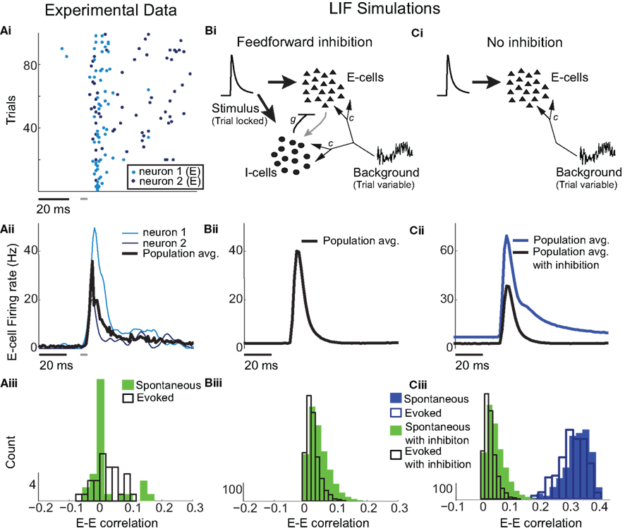
Figure 1. Low E-cell noise correlation in experiments and a model with feedforward inhibition. (Ai) Raster plot of paired E-cell activity across different trials (dark and light blue dots are from distinct neurons). Each trial contained a period of time before, during, and after whisker deflection. The duration of the whisker deflection is marked with a horizontal bar (after a time shift to account for feedforward propagation to L2/3). (Aii) Trial averaged firing rate; the dark and light blue curves correspond to the units in (Ai), and the black curve is the mean across all E-cells (n = 62). (Aiii) Distribution of ρ_EE values for distinct recorded pairs in spontaneous and evoked states (n = 31). The mean ρ_EE (across pairs) was 0.019 ± 0.06 in the spontaneous state and 0.023 ± 0.044 in the evoked state. (Bi) Schematic of the LIF L2/3 network with E and I-cell dynamics. On every trial each cell received inputs modeling L4 cell response to whisker deflection, with the temporal shape of the input matched to L4 responses and was trial locked. Each cell also received a trial variable low frequency Gaussian noise input modeling whisker independent synaptic input. These fluctuations were correlated across the network. (Bii) Trial averaged firing rate for the model with inhibition. (Biii) Distribution of ρ_EE values for different model neuron pairs in spontaneous and evoked states. Mean of ρ_EE was 0.03 ± 0.032 in the spontaneous state, and 0.024 ± 0.021 in the evoked state. (Ci) Schematic of the LIF L2/3 network with only E-cell dynamics. E-cells received the identical external inputs as in the case with inhibition. (Cii) Trial averaged firing rate for the model without inhibition. The model firing rate with inhibition is shown for comparison. (Ciii) Distribution of ρ_EE values for different model neuron pairs for the model without inhibition. The mean ρ_EE was 0.34 ± 0.047, in the spontaneous state, and 0.34 ± 0.044 in the evoked state. The model ρ_EE distribution with inhibition is shown for comparison.

E-cell spontaneous firing rate was 2.1 Hz (averaged across different neurons, n = 62), while whisker deflection caused a brief, yet substantial increase in the trial averaged firing rate to 34.6 Hz (Figure 1Aii). For a pair of E-cells the increase in firing rate during whisker deflection caused a large co-activation of spike responses (compare light and dark blue spike times in Figure 1Ai), consistent with past studies in somatosensory cortex (Kerr et al., 2007; Jadhav et al., 2009; Khatri et al., 2009). Despite these large firing rates, the probability of an E-cell firing within 30 ms of the whisker deflection was roughly 20%, indicating a large amount of response variability. The joint variability of a pair of E-cells was quantified with the correlation coefficient, ρ_EE, between their spike counts (computed over 30 ms sliding windows, see Materials and Methods). The spike count correlation coefficient is a standard metric used to measure population-wide variability (Zohary et al., 1994; Gawne et al., 1996; Kohn and Smith, 2005; Gutnisky and Dragoi, 2008; Smith and Kohn, 2008; Cohen and Maunsell, 2009; Mitchell et al., 2009; Ecker et al., 2010; Renart et al., 2010; Middleton et al., 2012), and quantifies correlations that are not attributable to the stimulus, yet are rather due to an internal cortical state that is variable from trial-to-trial. For our data ρ_EE was low (relative to what has been reported in pyramidal neurons, see Cohen and Kohn, 2011) in both the spontaneous and whisker evoked states – having average values across different E-E pairs of 0.019 and 0.023, respectively (Figure 1Aiii, n = 31 pairs). This indicated a near independent pairwise variability (assuming Gaussian statistics) between E-cell spike outputs. This result is surprising considering that whisker deflection evoked an order of magnitude change in the firing rates compared to spontaneous conditions. Uncovering the cellular and circuit mechanisms that produce the low value of ρ_EE, and its invariance across spontaneous and whisker evoked states, is the central aim of our study.

One possible explanation for low ρ_EE values is that the synaptic connections which provide input variability to pairs of E-cells have little overlap, so that the synaptic currents to the neuron pair are themselves uncorrelated. In this case, the low co-variability of spike train outputs would be inherited from the lack of correlation between the synaptic inputs to E-cell pairs. Poulet and Petersen (2008) and Gentet et al. (2010) performed simultaneous intracellular recordings from pyramidal neurons pairs in layer 2/3 of rodent somatosensory cortex. They reported significantly correlated membrane potential activity in spontaneous conditions, showing that the inputs to pyramidal cell pairs are in fact correlated. Nevertheless, despite this input correlation, their pyramidal cell spike trains showed similarly low correlations in the spontaneous state as in our recordings (see Gentet et al., 2010 their Figure 6B). In total, the results from Poulet and Petersen (2008) and Gentet et al. (2010) are inconsistent with the hypothesis that uncorrelated firing in the spontaneous state is a reflection of uncorrelated membrane potential fluctuations.

In our previous study (Middleton et al., 2012) we presented a firing rate model of layer 2/3 somatosensory cortex that replicated the experimentally observed correlated dynamics of E-cells in both the spontaneous and stimulus evoked state. A critical component of the model was a strong feedforward inhibitory component, known to shape the trial averaged response of pyramidal neurons in primary somatosensory cortex (Pinto et al., 1996, 2000; Miller et al., 2001). However, the phenomenological nature of firing rate models precluded a clear understanding of the mechanisms that determine actual pairwise spike train correlations. To test and expand upon the predictions of our past model, we implemented a leaky integrate-and-fire (LIF) model network of layer 2/3 somatosensory cortex, where a population of E-cells received a strong feedforward inhibition from a population of I-cells (see Materials and Methods and Figure 1Bi).

The model neurons (both E and I) had two sources of external synaptic input. The first was a Poisson train of excitatory inputs whose inhomogeneous firing rate was temporally matched to the firing rate responses from layer 4 neurons (which provide input to layer 2/3) in response to whisker deflection in previous studies (Pinto et al., 2000). The precise synaptic arrival times were uncorrelated between cells, yet the temporal evolution of the stimulus was identical for all neurons and fixed across stimulation trials (see Materials and Methods and Figure 1Bi inset). The transient nature of the input produced an elevated, trial averaged population firing rate during whisker input that matched the experimental data (Figure 1Bii). The second source of external input was a low frequency, Gaussian noise processes that was partially correlated between any pair of neurons. This input modeled a spatially broad local field potential previously shown to account for the pairwise firing statistics of both E and I-cells in spontaneous conditions (see Figure 5 of Middleton et al., 2012). The synaptic field potential was the source of trial-to-trial variability in our network model. The degree of correlation of this input was set so the model correlation ρ_EE matched that from our experiments, in both the spontaneous and whisker evoked conditions (Figure 1Biii with c = 0.5 throughout all LIF simulations, see Materials and Methods).

When inhibition was absent, there was a temporal broadening of the population firing rate (Figure 1Cii, cf. blue and black curves), consistent with results from firing rate models (Pinto et al., 2000; Miller et al., 2001; Bruno and Simons, 2002). However, feedforward inhibition was also crucial for maintaining the observed low ρ_EE correlation values in both spontaneous and evoked states. Indeed, without inhibition ρ_EE was unphysiologically large in the LIF simulations (Figure 1Ciii). In total, when a strong feedforward inhibitory component was present our LIF network replicated both the trial average response, and the trial-to-trial variability observed in our experimental results.

Whisker Velocity and E-E Correlation

Natural somatosensory processing produces a wide range of whisker velocities as rodents probe their environments (Ritt et al., 2008; Wolfe et al., 2008). The LIF model enabled simulation of the network response to whisker deflection with distinct whisker velocities. We varied the stimulus input in the spiking model based on recordings of layer 4 excitatory neurons responses to different velocities (Pinto et al., 2000). Briefly, as velocity increased (Figure 2A, left), the mean input rate peaked earlier and decayed faster (Figure 2A, right). For all whisker velocities, the temporal dynamic of the model evoked E-cell firing rate was much sharper with inhibition intact, compared to a network lacking inhibition (Figures 2Bi,Ci). For each whisker velocity V, we considered the time integrated response of the network following the onset of the stimulus divided by the spontaneous firing rate:

FIGURE 2

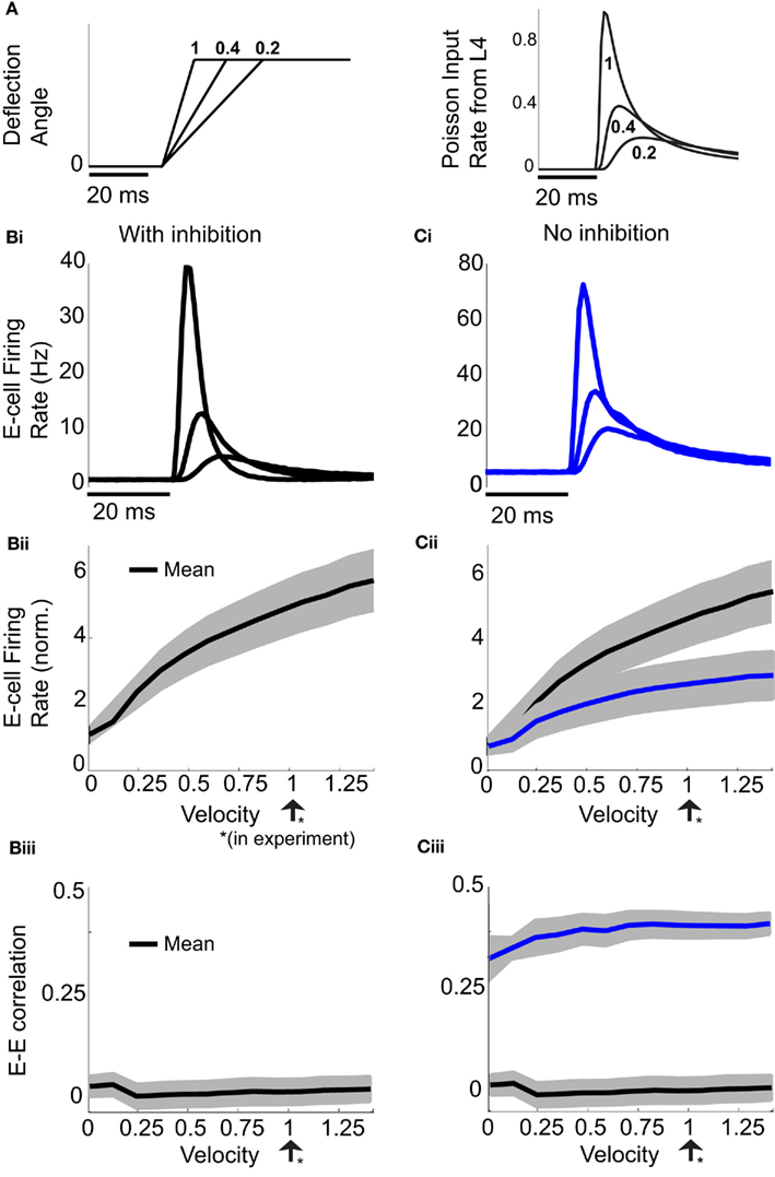
Figure 2. Effects of varying whisker deflection velocity in the spiking model. (A) Different time intervals to evoke a fixed deflection angle result in different whisker velocities (left). An increase in whisker velocity scales the peak and broadness the temporal waveform of L4 pyramidal cell responses (right), as reported in Pinto et al. (2000). A velocity of 1 corresponds to the value used in our experiments, two other smaller velocities are shown for comparison purposes. (Bi) The trial averaged E-cell firing rate in time in the model with inhibition for the same whisker input velocities in (A). (Ci) Same as (Bi) but for the model without inhibition. (Bii) The normalized E-cell firing rate (see equation (10)) as a function of velocity in the model with inhibition. (Cii) Same as (Bii) but for the model without inhibition. Model with inhibition is shown for comparison. Shaded regions represent mean ± 0.25 SD across different neurons. (Biii) With inhibition, ρ_EE is approximately constant and small across a large range of velocities. (Ciii) Without inhibition, ρ_EE is much larger (cf. blue with black curve) – shaded regions represent mean ± SD across different neuron pairs.

Here v_E(t) is the population firing rate, T₀ is the onset time of the whisker stimulation, and T = 30 ms (the same time window used to measure the spike count correlations). Thus defined r_E(V) measures the normalized sensitivity of the population response to whisker velocity. A velocity of V = 0 corresponds to the spontaneous state (so that r_E(0) = 1), while a velocity of V = 1 is when the model best matched the whisker evoked experimental data (Figure 2Bii).

Not surprisingly, r_E(V) increased with velocity. However, the removal of feedforward inhibition decreased the velocity sensitivity of the normalized response r_E (Figure 2Cii, blue is below the black curve). The large response sensitivity with inhibition intact was due to the suppression of firing rate during spontaneous conditions, while transient whisker responses escaped a delayed feedforward inhibition and was thus not suppressed (Pinto et al., 2000). While inhibition enhanced the trial averaged E-cell sensitivity to whisker velocity, it also had a large impact on the trial-to-trial variability of the population response. When inhibition was present ρ_EE was consistently low over a large range of whisker velocities (Figure 2Biii). This is in contrast to a model without inhibition where ρ_EE was much larger (Figure 2Ciii, blue is above the black curve). Thus, feedforward inhibition both increased population response sensitivity to whisker velocity and reduced pairwise co-variability over a range of evoked states. While the former has been the focus of several studies (Pinto et al., 2000; Miller et al., 2001), the observation that feedforward inhibition maintains low correlated variability is novel, and the mechanisms that support this are the topic of the next sections.

Simplified Binary Neuron Model Network

The LIF network replicated our experimental recordings and predicted that a feedforward inhibitory path is required for low correlated trial-to-trial variability of the E-cell population spiking activity. However, the complexity of the spiking model simulations made further analysis difficult. Following past work (Ginzburg and Sompolinsky, 1994; Renart et al., 2010), we highlight the core mechanisms underlying our model predictions by considering a simplified network where LIF neuron models were replaced with non-dynamic, two-state binary neuron models (see Materials and Methods). Briefly, on every stimulus trial each binary neuron model received a random input, and outputted a response that was either a 0 (no spike) or a 1 (a spike), depending on if the input was below or above a threshold value θ, respectively (Figure 3Ai). Input variability was Gaussian distributed for I-cells (Figure 3Ai, top). For E-cells the input was the combination of a Gaussian distributed field and the binomial responses from a subset of the I-cell population, scaled by −g, that project feedforward to the E-cell (Figure 3Ai, bottom). As in the LIF simulations, the synaptic field inputs were correlated with strength c for all cell pairs (E-E, E-I, and I-I).

FIGURE 3

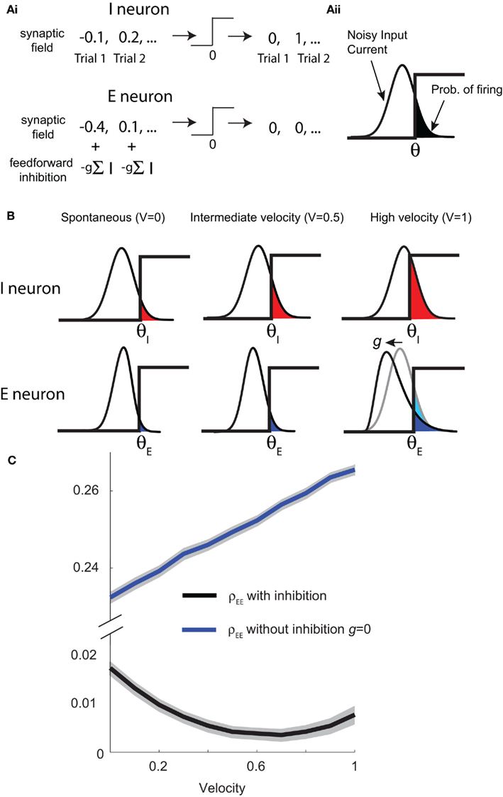
Figure 3. Binary network capture E-cell statistics. (Ai) Binary neuron model receives random drive from the synaptic field (assumed to be Gaussian) on a given trial, resulting in a “spike” (denoted by a 1) if the total input is above threshold or no response (denoted by a 0) if the total input is below threshold. I neuron (top) only receives input from the synaptic field whereas an E neuron (bottom) also receives feedforward inhibitory input. (Aii) The probability of a response on a given trial is the area of the input probability density above threshold θ. An increase in whisker velocity is modeled by a decrease in threshold θ. (B) The probability of spiking (colored region: red for I neuron, blue for E neuron) increases with velocity (left to right). The effect of inhibition on the excitatory neuron is demonstrated with high velocity (lower right, V = 1). (C) A large binary network consisting of 50 excitatory neurons, each receiving a random number of inhibitory inputs (avg. 118), qualitatively captures the average correlation (as well as other statistics, see Figure S2 in Supplementary Material). Across a range of velocities, ρ_EE remains consistently low with inhibition (black), but dramatically increases without inhibition (blue). Shaded regions represent mean ± SD across different neuron pairs.

For binary neuron models the response probability is the fraction of the input probability density that is larger than the threshold (Figure 3Aii, shaded region). Since the stimulus was fixed across trials, a change in whisker velocity resulted in a shift of the input density by a deterministic amount, applied to both the E and I neurons (Figure 3B, left to right). Equivalently, an increase in whisker velocity can be thought of as a decrease in threshold θ, and in the model we made the association θeta = θ₀ − kV, where V is whisker velocity and k > 0 is a linear scaling. For the I-cell population the input variability was Gaussian distributed for all whisker velocities (Figure 3B, top), while the input distribution to E neurons was not Gaussian because of the variability of the feedforward I-cell activity. This variability was significant for large whisker velocities, skewing the distribution of total E-cell inputs (Figure 3B, bottom-right). Nonetheless, the feedforward architecture allowed a calculation of the joint “spiking” statistics of the network using thresholded high dimensional Gaussians (i.e., dichotomized Gaussians; see Appendix). We computed the spike statistics from a large feedforward binary network (50 excitatory neurons each receiving an avg. of 118 inhibitory inputs). The E-cell population showed low ρ_EE across a range of whisker velocities (Figure 3C, black curve). Furthermore, ρ_EE was much larger without inhibition (Figure 3C, blue curve; note the broken axis). Thus, despite the simplifications from the LIF network, the binary network model with inhibition exhibited low E-E cell co-variability over a broad range of activation, similar to LIF spiking model and the experimental data (Figure 3C; Figure S2 in Supplementary Material). Further, its analytic tractability allowed for a deeper analysis of the mechanisms that maintain low E-E co-variability, which we present below.

To ease presentation we analyzed a small network of two E-cells receiving feedforward inhibition from one I-cell. Further, we focused on the response covariance rather than the correlation coefficient ρ; this simplification did not qualitatively impact our results since the near zero ρ_EE is due to spike count covariance being small, as opposed to variance being excessively large. The response statistics of the E-E pair obeyed:

where G_n is an n-dimensional Gaussian with 0 mean, unit variances, and covariances of strength c (see equations (A29)–(A31) in Appendix). Variables x and y_j are the distribution values of the synaptic field to the inhibitory and excitatory neurons, respectively. We remark that the strength of feedforward inhibition, g, only appears in the limits of the integrals, implying that inhibition acts to effectively raise E-cell threshold. How Cov_EE depends on our key parameters g, c, and θ is not obvious or transparent. Thus, we considered the asymptotic limit of small c and g and derived the following compact approximation for Cov_EE (see cf. equation (A34) in Appendix with σ_E = σ_I = 1):

with

Here the I-cell response probability is Equation (14) is one of our main theoretical results, and offers a framework to understand the mechanism that maintain low ρ_EE over a range of stimulus intensities.

Equation (14) shows that the output covariance Cov_EE factorizes into the product of the input covariance Cov_in and the E-cell covariance susceptibility S. The susceptibility S ∈ [0, 1/2π] measures the linear relationship between input and output co-variability. A truly linear system (meaning the output is simply a scaled version of the input) has S = 1, while in general a non-linearity in the input/output transfer reduces S, as is the case for spiking neurons (de la Rocha et al., 2007). For binary models S = 1/2π is maximized when θ_E = 0; here the input distribution maximally straddles the threshold so that fluctuations are best transferred and there is minimal correlation dilution. Decomposing Cov_EE as in equation (14) was motivated by studies of pairs of uncoupled cells (de la Rocha et al., 2007; Marella and Ermentrout, 2008; Shea-Brown et al., 2008; Barreiro et al., 2010; Tchumatchenko et al., 2010; Litwin-Kumar et al., 2011; Rosenbaum and Josić, 2011); however, in equation (14) we have expanded the framework to capture our feedforward circuit model. To gain insight in how Cov_EE is maintained at low values over a range of stimulus intensity, we explored equation (14) by a process of gradually building our simplified circuit model to match the criteria of the full model.

Correlation Dilution and Cancelation Balance to Maintain Low E-E Covariance

We first considered a pair of E-cells subject to a correlated synaptic field (c > 0), yet with feedforward inhibition removed (g = 0), so that the correlation transfer reduced to its simplest case (Figure 4Ai). Here the total input covariance was Cov_in = c, so that Cov_in was velocity independent (Figure 4Aiii, black curve). In contrast, the covariance susceptibility S was velocity dependent through the E-cell response threshold θ_E. For small velocities, θ_E > 0 was large, making small, implying that the transfer of co-variability was poor (Figure 4Aiii, red curve). This is because the threshold non-linearity of the binary model attenuated the overall transfer of inputs. When the whisker velocity increased so that θ_E decreased, thresholding was less effective at suppressing fluctuations meaning S increased (Figure 4Aiii, red curve). The increase in S subsequently caused Cov_EE to increase (Figure 4Aiii, green curve). Due to the multiplicative nature of S on Cov_in we termed mechanisms that affect co-variability through S as correlation dilution.

FIGURE 4

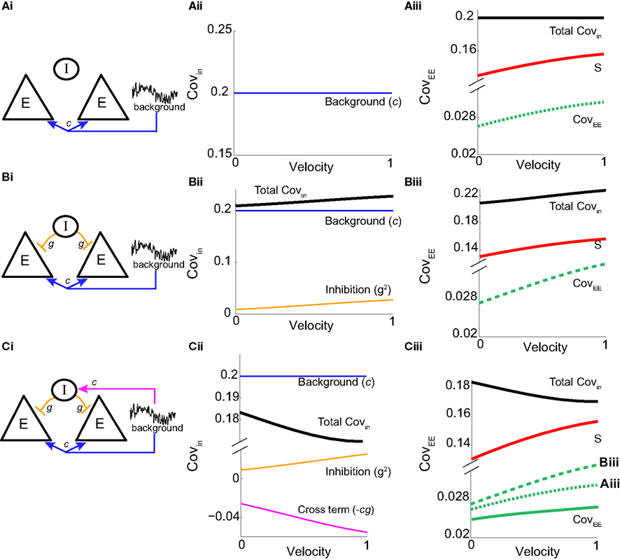
Figure 4. Mechanism for low E-E co-variability. Analysis of a small binary network (2 E and 1 I) shows how the output covariance depends on the input covariance and threshold non-linearity: Cov_EE ≈ SCov_in (equation (14)). (Ai) Schematic of a network with no inhibition where the pair of E-cells receive common background input. (Aii) The input covariance is Cov_in = c (equation (14) with g = 0), and independent of velocity. (Aiii) The susceptibility function (red) increases with velocity (i.e., decreases with threshold), so that the output covariance Cov_EE ≈ Sc (green) also increases with velocity. (Bi) A network that now includes inhibition where the I-cell does not receive input correlated to the E-cells. (Bii) The input covariance consists of two terms: c (blue) and 2g²v_I (1 − v_I) (orange). In total, Cov_in = c + 2g²v_I (1 − v_I) (black) increases with velocity. (Biii) Cov_EE (green) is even larger (more synchronous) than in (Aiii) because both S and Cov_in increase with velocity. (Ci) A network that now includes correlated input to all cells. (Cii) The input covariance consists of three terms: c (blue), 2g²v_I (1 − v_I) (orange), and a negative cross term (magenta) that decreases with velocity. The total input covariance (black) decreases with velocity. (Ciii) S (red) increases with velocity while Cov_in (black) decreases with velocity, maintaining an approximately constant and low spike count covariance Cov_EE ≈ SCov_in for all velocities (solid green) compared to (Aiii) (dotted green) and (Biii) (dashed green).

We next considered a circuit with feedforward inhibitory coupling intact, but where the noisy synaptic field inputs that gave rise to E-E correlation were uncorrelated with those provided to the I neuron (Figure 4Bi). This network had the first two terms of Cov_in, but not the cross term (proportional to cg) in equation (14), yielding Cov_in = c + g²2v _I(1 − v _I). The first term was again due to a correlated synaptic field, while the second term was due to the projections from the common I-cell to the E-cell pair. While the synaptic field continued to be independent of velocity (Figure 4Bii, blue curve), the amount of feedforward inhibition recruited increased with velocity due to v_I’s dependence on θ_I (Figure 4Bii, orange curve). This was because the thresholding of the I neuron attenuated the co-variability that correlated inhibition provides, and this impact of the threshold was reduced when θ_I decreased. In total, Cov_in increased with velocity (Figure 4Bii, black curve). When Cov_in was multiplied by the susceptibility S, Cov_EE increased significantly with velocity, and was larger than the case when inhibition was removed (Figure 4Biii, green curve; verified in the LIF spiking model in Figure S3 in Supplementary Material). This network is consistent with the idea that inhibition can lead to synchrony (i.e., higher correlation in a small time window; van Vreeswijk et al., 1994; Wang and Buzsáki, 1996; Whittington et al., 2000; Cardin et al., 2009).

Finally, if the same correlated background input for the excitatory neurons also provided input to the inhibitory neurons (Figure 4Ci), the output covariance was approximated by the full equation (14). This circuit captured the key aspects of our LIF network (Figures 1 and 2). The inclusion of the negative cross term (magenta line in Figure 4Cii) opposed the contributions of the first and second terms, such that Cov_in now decreased as velocity increases (black line in Figure 4Cii). Due to the subtractive aspect of the third term in equation (14) we termed the overall mechanism correlation cancelation. This scheme is similar to mechanisms proposed in recurrent cortical networks, where dense, balanced activity maintains an overall low level of input correlation (Renart et al., 2010).

The decrease in Cov_in was countered by an increase in S as velocity ranged from small to large values (Figure 4Ciii, red and black lines). In total, Cov_EE ≈ SCov_in was maintained at a near constant level over a wide range of stimulus intensities (Figure 4Ciii, green line; Cov_EE for the other networks are plotted for comparison; they are relatively larger and increase more with velocity). Thus, we propose that the combination of cancelation of correlation via feedforward inhibition and correlation dilution via S was such that E-E response co-variability changed very little as whisker velocity changed. Binary model neurons are oversimplified and cannot quantitatively capture the complicated dynamics of real spiking model systems. Nevertheless, the analysis presented here is a proof of principle that gave some clear predictions that we could test in our LIF spiking model network.

Correlation Dilution and Cancelation in the LIF Model

Our binary model network suggested we measure the stimulus-induced changes of both Cov_in and S for the E-cell pairs in the spiking model network. To do this we first decomposed the total input to every E-cell (Figure 5A, black curves) as the sum of the background synaptic field (Figure 5A, blue curves) and the feedforward inhibition (Figure 5A, orange curves). We computed the covariance statistics of the input fluctuations across trials and pairs in our network. As expected, the covariance of background synaptic field was both high and independent of whisker input (Figure 5B, blue curve). This contrasted with the low covariance of the inhibitory inputs to a pair of E-cells during spontaneous conditions, which rose sharply with whisker input (Figure 5B, orange curve). This was because the firing rates of the I-cells increased significantly during stimulus presentation, and hence so did the co-variability of inhibition to the E-cells. However, when both background and inhibition were combined, the total input covariance decreased during stimulus presentation (Figure 5B, black curve). Thus, the correlation cancelation via feedforward inhibition illustrated with the binary network (Figure 4Cii) occurred in the more complicated LIF model system. Furthermore, in agreement with past results (de la Rocha et al., 2007), the covariance susceptibility S of our model LIF neurons receiving a weakly correlated fluctuating input increased over the range of firing rates experienced during whisker stimulation (Figure 5C). In total, our LIF network exhibited a combination of correlation dilution and cancelation, as first observed in binary model neuron network (Figure 4C).

FIGURE 5

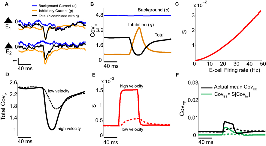
Figure 5. Validation of binary model analysis with the LIF spiking model. (A) The input currents are dissected into background I_c(t) (blue) and inhibitory synaptic I_g(t) (orange) components: I_total(t) = I_c(t) + I_g(t) (black). A single realization for a pair of E-cells is shown with V = 1. (B) The covariance of the input currents, averaged across pairs, has the following features: the input covariance from the background is constant (blue), the inhibitory synaptic input’s covariance increases with firing rate (orange), but together the total input covariance decreases with firing rate (black) – cf. Figure 4Cii. (C) The covariance susceptibility function S for the LIF spiking model increases with firing rate. (D) The input covariance for a low (dashed, V = 0.1) and high velocity (solid, V = 1) whisker input in time decreases by different amounts upon whisker stimulation. (E) The susceptibility function in time is determined by the instantaneous firing rate [interpolating the curve in (C)]; low velocities have smaller S and higher velocities have larger S. (F) The approximation of the spike count covariance in green, obtained by multiplying corresponding black and red curves, is small like the actual Cov_EE (cf. Figure 4Ciii). The dashed-lines correspond to low velocity, solid lines correspond to high velocity.

We next verified with our spiking model network that this combination of correlation dilution and cancelation maintained low E-E co-variability over a range of whisker velocities. The decrease of the total input covariance during whisker stimulation, relative to spontaneous conditions, was larger for high velocity stimuli than that for low velocity stimuli (Figure 5D, solid vs. dashed). However, the increase in E-cell firing rate for high versus low velocity stimuli caused the covariance susceptibility to be larger for the high velocity input (Figure 5E, solid vs. dashed). Motivated by the results from our simplified binary model network, we computed an approximation to Cov_EE obtained by multiplying the total input covariance and the susceptibility (Figure 5F, green), and saw that the result was similar to the actual Cov_EE (Figure 5F, black). We remark that in the LIF network without inhibition, the Cov_EE values ranged from 0.025 to 0.065 (not shown), which was much larger than the results with inhibition intact (Figure 5F), consistent with our binary network results when g = 0 (Figure 4A). The results from our LIF simulations support our general theory that over a range of stimuli intensities high total input covariances were balanced by low S values, while high S values were balanced by low total input covariances.

Consequences for I-E Correlation

In the LIF network we chose c and g values to be relatively large in order to capture the low ρ_EE values across a range of velocities. With a large (c, g) pair, a precise relation between c and g is needed for a low value of ρ_EE, since if we set either c to zero (between E and I, Figure S3 in Supplementary Material) or g to zero (Figure 1C) the co-variability increased significantly. However, low ρ_EE can also be obtained by simultaneously decreasing the strength of both c and g, effectively attenuating all sources of co-variability. Thus, a specific choice of the (c, g) pair would not be required to guarantee a low ρ_EE. We therefore needed testable predictions that clearly distinguish between our mechanism of correlation dilution and cancelation produced by a large (c, g) pair and a mechanism based on the simple lack of correlation given by small (c, g) pairing.

For a given whisker velocity in the small binary network there was a family of (c, g) values for equation (14) that lead to Cov_EE ≈ 0. For a collection of fixed velocities (ranging between 0 and 1, see Figure 4) the (c, g) pairs that achieve Cov_EE ≈ 0 were generally in a diagonal region of parameter space (one gray line per velocity in Figure 6A). An asymptotic approximation for Cov_IE in a small binary network consisting of one excitatory and one inhibitory neuron, similar to equation (14), enabled an efficient exploration of the effect of particular (c, g) values on Cov_IE. Our calculations (see cf. equation (A36) in Appendix) resulted in the following:

FIGURE 6

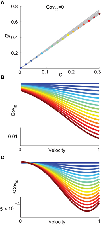
Figure 6. Analysis of I-E statistics in the binary model. (A) With the analytic approximation for Cov_EE (equation (14)), we plot the region of parameter space (c, g) where Cov_EE ≈ 0, with each gray line representing a particular velocity (ranging from 0 to 1, see Figure 4). Larger values of c correspond to larger g values. Color-coded dots are a representative subset of (c, g) pairs used below in (B,C). (B) The analytic formula for Cov_IE (equation (15)) enables analysis of how it changes with velocity for a particular pair of c and g values (colored coded). Although many (c, g) pairs give Cov_EE ≈ 0, larger values exhibit more of a decrease in Cov_IE with velocity (the decrease is of the same order as the full binary network and LIF simulations). (C) A similar analysis for the width of the histogram of Cov_IE (see equation (16)) values, again, shows that large c and g values correspond to more of a decrease in the width of this distribution in the evoked state. Except for c and g, the parameters for the binary model match those used in (Figure 4).

We chose a representative subset of (c, g) pairs (color-coded in Figure 6A) and substituted these into equation (15) to study the dependence of Cov_IE on whisker velocity. Although all (c, g) pairs produced Cov_EE = 0, larger (c, g) values resulted in a appreciable decrease of Cov_IE when velocity increased from low to high values (Figure 6B). This is because the term becomes more negative as θ_I decreases, effectively anti-correlating E and I-cell activity as whisker velocity increased. Of course, for small c and g, Cov_IE is also small and independent of whisker velocity. In total, this analysis shows that the invariance of Cov_EE to whisker velocity produced by a large (c, g) pair does not hold for Cov_IE.

We further considered how the spread of Cov_IE values in a heterogeneous network changed with whisker velocity. We analyzed a small binary network consisting of two heterogeneous inhibitory neurons having (see Appendix) providing feedforward input to a single excitatory neuron. We measured heterogeneity of Cov_IE by taking the difference yielding the result (see cf. equation (A43) in Appendix):

where We substituted (c, g) values that gave Cov_EE ≈ 0 (color-coded in Figure 6A) into equation (16), and saw that larger (c, g) values showed a significant decrease in ΔCov_IE when velocities ranged from low to high values.

In total, these analyses provided two clear signatures of a large (c, g) pairing for I-E response statistics:

1. Cov_IE measured during spontaneous conditions will be larger than that measured during stimulus evoked conditions.

2. The spread of Cov_IE in a heterogeneous network of E and I-cells will be larger when measured during spontaneous than during stimulus evoked conditions.

We next tested these two predictions with both the LIF spiking model simulations and simultaneously recorded E and I activity from layer 2/3 of somatosensory cortex.

Our experimental data set not only contained E-E pairs (Figure 1A), but we also obtained a large number of I-E pairs (n = 48), allowing us to measure the co-variability of excitatory and inhibitory spiking (Middleton et al., 2012). In somatosensory cortex, fast spiking inhibitory neurons have larger spontaneous and peak-evoked firing rates than excitatory neurons (Bruno and Simons, 2002; Swadlow, 2003; Middleton et al., 2012), evident in both the LIF simulations (Figure 7Ai) and the experimental data (Figure 7Bi). In agreement with our predictions for large (c, g) pairing, both the average ρ_IE and the spread of ρ_IE around the average computed from the LIF network (Figure 7Aii) and the experimental recording (Figure 7Bii) decreased in the whisker evoked state compared to the spontaneous state. Further, the decrease in the mean of ρ_IE is observed not only in the population response, but also on a pair-by pair basis for both the networks simulations and experimental recordings (Figure 7C). In the LIF model this indirect test of the consequences of a large (c, g) values, while it verifies our binary model predictions (Figure 6), is not strictly required since we can set either c or g to zero and observe the direct shifts in network co-variability expected for a large (c, g) pairing (Figure 1Ciii for g = 0 and Figure S3 in Supplementary Material for uncorrelated E and I activity). However, such a direct test was not an option in the experimental recording, as manipulations of g and c were not possible. Thus, the fact that our experiments were in line with our predictions (1, 2) is compelling evidence that the invariance of ρ_EE for real layer 2/3 cortical response (Figure 1Aiii) is due to a combination of correlation dilution and cancelation in a cortical network with strong feedforward inhibition.

FIGURE 7

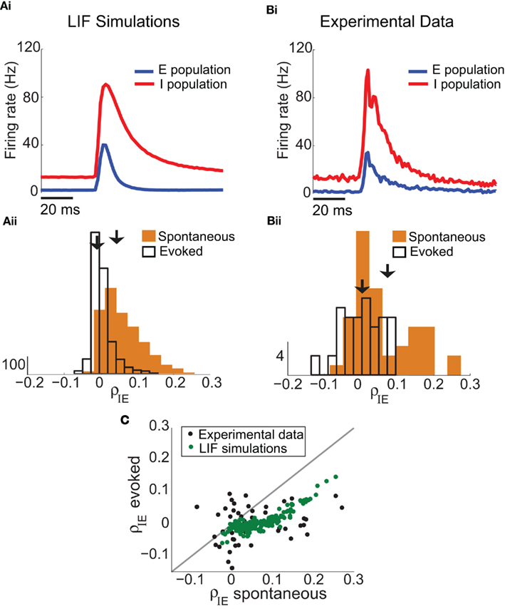
Figure 7. I-E subnetwork statistics in the LIF model and experimental data. (Ai) In the model with inhibition (same network as Figure 1B), the firing rate of the I-cells (red) is larger than the E-cells (blue). (Bi) In the experimental data, the firing rates of the I-cells are larger (v_I,spont = 13.6 Hz and v_I,evoked = 103 Hz with n = 48 I-cells). (Aii) In the spiking model with feedforward inhibition, the mean of ρ_IE is 0.59 (SD of 0.053) in the spontaneous state, and decreases to ρ_IE = − 0.0026 (SD of 0.028) in the evoked state. This is consistent with the binary analysis prediction in (Figure 6B,C) because the value of c and g are relatively large. (Bii) In the experimental data, the mean of ρ_IE is 0.057 (SD of 0.083) in the spontaneous state, with a mean ρ_IE of 0.0009 (SD of 0.056) in the evoked state. The data shows a decrease in ρ_IE in the evoked state compared to the spontaneous state, and a decrease in the width of the histogram of ρ_IE values (n = 48 I-E cell pairs). (C) Decrease in ρ_IE holds across pairs: the decrease is larger with whisker stimulation when spontaneous ρ_IE is larger in both experimental data (black dots) and the LIF spiking model (dark green dots).

Consequences for Coding

Rodents rely heavily on their whiskers for sensing and must be able to distinguish many different velocities encountered in their environment (Ritt et al., 2008; Wolfe et al., 2008). Transient whisker deflections are due to a “stick-slip” whisker dynamic when whiskers interact with an object, and the velocity of the whisker deflection is heavily dependent on the texture of an object. Behavioral studies show that rodents use their whiskers to make discriminations of fine texture differences (Guic-Robles et al., 1989; Carvell and Simons, 1990), suggesting a neural representation of whisker velocity. Indeed, recordings from barrel cortex have established that deflection velocity, as opposed to simply whisker deflection frequency or amplitude, is well represented by both single units (Wang et al., 2010) and the joint response of populations of neurons (Arabzadeh et al., 2003, 2004; Jadhav et al., 2009). We next focused on the information content about whisker velocity contained in the responses of the excitatory neuron population. In particular, we investigated the impact that feedforward inhibition had on the population code, given its role in both enhancing response sensitivity (Figure 2Cii) and reducing E-E cell co-variability (Figure 2Ciii).

To measure the confidence in the estimate of whisker velocity from single trial population spiking activity, we use the linear Fisher information J (Kay, 1993) computed from the E-cell spiking activity. The inverse of J is the lower bound on the error for the optimal linear estimator of the velocity (Kay, 1993), and thus a larger J indicates a better overall velocity code. For our network, we have:

where r _E is the vector of population responses of the excitatory neurons, the notative “′” denotes differentiation with respect to velocity, and Q is the covariance matrix of spike counts in the 30-ms time window upon a whisker deflection. For populations with distributed responses tuning, such as visual cortex representations of stimulus orientation or color, estimates of Q from spiking networks can be cumbersome (Seriès et al., 2004). However in our network, all neurons responded similarly to increases in velocity, with response heterogeneity arising only from random network architecture and spike threshold values. This fact, coupled with the smaller size of our E-cell network (N_e = 200) enabled more direct estimates of Q. For computational efficiency, only about 10% of the possible pairs of covariance values were stored, the rest of which were randomly sampled until Q was positive semi-definite (see Figure S4 in Supplementary Material for details). The reported J/N_e has been averaged over realizations of Q. In considering the linear Fisher information we neglected any codes based on the variability of population response (Shamir and Sompolinsky, 2004), however a linear J can be estimated from spiking responses (Seriès et al., 2004; Beck et al., 2011) and serves as a reasonable measure of coding performance when knowledge of higher order responses statistics (i.e., 3rd and above) cannot be obtained (Beck et al., 2011).

Over the entire range of velocities, the network with feedforward inhibition had Fisher information values that were roughy two orders of magnitude larger than those from a network without inhibition (Figure 8A). To highlight the mechanisms by which feedforward inhibition enhanced population codes we dissected the contributions of inhibition to J. Response sensitivity was measured by or loosely the “slope” of the trial averaged E-cell evoked firing rate versus whisker velocity. equation (17) shows that J increases as does. On the other hand, response variability was measured by Q, and for populations of neurons with similar stimulus tuning J will generally decrease as ||Q|| increases (Abbott and Dayan, 1999; Sompolinsky et al., 2001; Josic et al., 2009). In our network inhibition both increased response sensitivity (Figure 2Cii) and provided mechanisms of low E-E co-variability (Figure 2Ciii), thus we expect a synergistic effect of inhibition on population codes. The Fisher information J computed with the Q⁻¹ obtained from the network with inhibition (smaller covariances), but with response vector obtained from the network without inhibition (smaller sensitivity), was intermediate between the information computed from simulations with and without inhibition (Figure 8B, black dashed curve). In a similar fashion, the information obtained when we use the Q⁻¹ from the network without inhibition (larger covariances) and the response from the network with inhibition (larger sensitivity) was also intermediate to that computed with or without inhibition (Figure 8B, blue dashed curve). Both dashed curves do not correspond to an actual network response because second order statistics Q depend on first order statistics r _E, and as such do not represent a realizable neural code. However, they do quantify how important both inhibition enhanced sensitivity and inhibition mediated decorrelation are for an accurate population code.

FIGURE 8

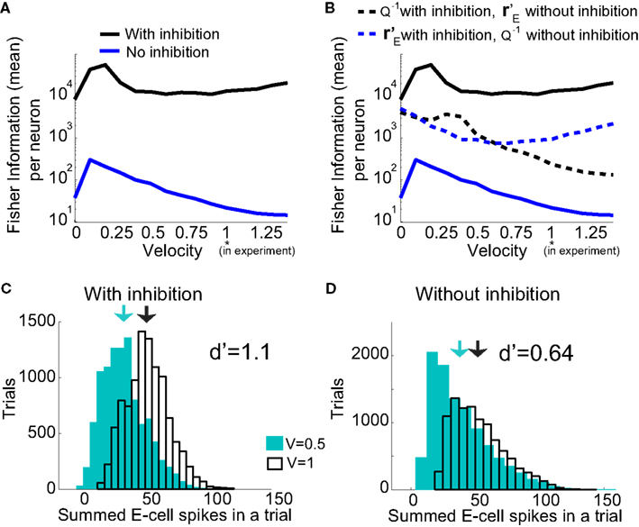
Figure 8. Fisher Information of the LIF model for varying velocities. (A) The Fisher information, per neuron, for the population response of the LIF spiking network model is much larger with inhibition (black) than without (blue); “′” denotes differentiation with respect to velocity. The network with inhibition has lower correlation, leading to larger ||Q⁻¹||, and is also more sensitive to velocity (i.e., larger values). The y-axis is a log-scale. (B) The black dashed curve is the Fisher information with Q⁻¹ obtained from the network with inhibition (low correlation), but with firing rate vector obtained from the network without inhibition. The dashed blue curve is Q⁻¹ obtained from the network without inhibition, and firing rates obtained from the network with inhibition. Although the dashed curves do not correspond to an actual network (Q and r_E are related), this shows how important both are for the difference in Fisher information because both dashed curves lie between the two solid curves. (C), Histogram of a weighted sum of E-cell spike counts during whisker stimulation (30 ms window) across trials of the model network with inhibition, for two different velocities: V = 0.5, 1. The discriminability, is relatively high: d′ = 1.1. (D) Same as C except for the network model without inhibition. The discriminability is much worse d′ = 0.64 due to high co-variability and less sensitivity to velocity.

To provide a concrete example for how inhibition enhances coding we performed a linear discriminant analysis (Duda et al., 2001) of the population responses when the velocity V was either 0.5 or 1. We take our linear code to be where a is a vector of weights that sets the contribution of the various cell responses to an overall population code. This effectively assumes a straightforward decoding of population activity, as might be expected by a neuron that receives weighted convergent input from the E-cell network. We computed the optimal weights (Duda et al., 2001) for the population discrimination (Fisher’s linear discriminant), yielding a = (Q₁ + Q_0.5)⁻¹(v₁ − v_0.5), where v_x and Q_x are the mean and covariance of the population response to velocity x. The network with inhibition produced a discriminable response based on trial distributions of V_est for the two velocities (Figure 8C), while the discrimination power of the population without inhibition was severely diminished (Figure 8D). The distribution of V_est from the networks showed that inhibition both separated the trial average responses, as well as reduced the variance of the responses, leading to an overall enhanced discrimination. In total, feedforward inhibition increased the whisker velocity estimation and discrimination power of stochastic networks of spiking neurons.

Discussion

Summary of Results

Co-variability of population activity across stimulation trials has been an intense focus of research (Averbeck et al., 2006; Faisal et al., 2008; Cohen and Kohn, 2011) with conflicting reports (Averbeck et al., 2006; Greenberg et al., 2008; Gutnisky and Dragoi, 2008; Smith and Kohn, 2008; Cohen and Maunsell, 2009; Mitchell et al., 2009; Ecker et al., 2010; Renart et al., 2010; Middleton et al., 2012). To provide greater insight into how cortical circuitry determines spike count co-variability across a range of network activation we expanded on our past study (Middleton et al., 2012) and utilized in vivo extracellular recordings, computational modeling, and theoretical analysis to study the rat barrel somatosensory cortex under whisker stimulation. We found that despite strong evidence for highly correlated background inputs to all neurons in layer 2/3 of the somatosensory cortex (Poulet and Petersen, 2008; Gentet et al., 2010), there were consistently low levels of E-E spike count correlation during both spontaneous and whisker evoked states. A feedforward inhibitory spiking network model captured the correlation structure of the experimental recordings, and motivated the study of a reduced binary model network. Using a binary model network we decomposed the mechanism that provided low co-variability to a combination of a spike threshold based correlation dilution for low levels of network activation and a circuit-based cancelation of correlation at high levels of network activity. Our analysis made clear predictions for how co-variability of I-E pairs would change with whisker input, and these were verified in simulation and experiment. Finally, the inhibition induced low E-Eco-variability and enhanced population sensitivity cooperated to dramatically increase the (Fisher) information content about whisker velocity.

Correlation Dilution and Cancelation in Somatosensory Cortex

Our study suggests that the low co-variability of E-cell activity (Figure 1) is due to a combination of correlation dilution through cellular excitability at low firing rates, and network-based correlation cancelation mechanisms at high rates. Our previous study (Middleton et al., 2012) presented a firing rate model that captured the essential features of our data, yet the model was not decomposed into the base mechanisms of correlation dilution and cancelation. Thus, our binary model treatment has provided novel insights and ties together not only our experimental data (Middleton et al., 2012), but also the work from several groups recording from populations of cells in superficial layers of somatosensory cortex.

Poulet and Petersen (2008) and Gentet et al. (2010) measured high membrane potential co-variability between E-E pairs, yet zero co-variability of E-E spikes in the spontaneous state. In the spontaneous state of our model, the synaptic field correlations were not canceled by feedforward inhibition, so that the membrane potential co-variability was significant (evident by Cov_in > 0). Nonetheless, correlation dilution via spike thresholding accounted for the low spike variability in spontaneous conditions. Moreover, Gentet et al. (2010) also report that the co-variability of I-E spike counts is larger than that of E-E spike counts in the spontaneous state. This was also the case in our model, since I-cells fired at a higher rate in the spontaneous state so that the correlation dilution mechanism was less effective than for a pair of low rate E-cells. Thus, a correlation dilution mechanism is consistent with both the high correlation of membrane potential activity and the low correlation of the spiking activity observed in the low rate spontaneous state.

The correlation cancelation mechanism employed in our study required that correlated excitatory inputs were canceled by correlated inhibitory inputs. This is consistent with estimates of the co-variability of excitatory and inhibitory inputs to pairs of pyramidal neurons in barrel cortex (Okun and Lampl, 2008), namely that excitatory and inhibitory currents are strongly anti-correlated. The fact that in our model correlation cancelation operated best in the stimulus evoked state also agrees with population recordings in somatosensory cortex showing that the trial-to-trial co-variability of simultaneously recorded cells plays a negligible role in population representation of whisker velocity (Petersen et al., 2001; Jadhav et al., 2009). However, a clear verification of correlation cancelation for high levels of network activations would require intracellular recordings from excitatory neuron pairs showing that the co-variability of inputs decreases with stimulus intensity. This prediction has yet to be tested in layer 2/3 of the rat somatosensory cortex. However, it is consistent with intracellular membrane potential recordings from simultaneously recorded pyramidal neurons in visual cortex, where a marked decrease in membrane potential co-variability is reported when stimuli with preferred orientation are presented, compared to that for blank stimuli (Yu and Ferster, 2010). Thus, we propose that in the superficial layers of somatosensory cortex a strong feedforward inhibitory circuit supports a correlation cancelation mechanisms which ensures that co-variability is low for stimulus evoked regimes.

Decorrelated Cortical Activity and Whisker Velocity Coding

Feedforward inhibition is a central component in many cortical circuits and is critical for several aspects of neural processing (Ferster and Miller, 2000; Bruno and Simons, 2002; Swadlow, 2003; Wehr and Zador, 2003; Wilent and Contreras, 2005; Higley and Contreras, 2006; Heiss et al., 2008; Priebe and Ferster, 2008; Cafaro and Rieke, 2010). In the barrel cortex, feedforward inhibition is associated with increased sensitivity of cortical responses to whisker velocity (Pinto et al., 2000; Miller et al., 2001; Bruno and Simons, 2002). These reports considered the trial averaged firing rate, and while it is an important descriptor of cortical response, any measure of coding must also consider the trial variability about the average (i.e., the noise). Correlated variability across a neuron population (i.e., noise correlation) has been shown to be weak in barrel cortex and hence contributes in a negligible fashion to sensory coding (Petersen et al., 2001; Arabzadeh et al., 2003, 2004; Jadhav et al., 2009). This may lead some to discount the relevancy of noise correlations in somatosensory codes. In our study we show that the mechanisms that maintain low noise correlations should not be dismissed, and rather require a matching of excitability and circuit-based mechanisms to decorrelate population variability across a range of stimulus intensities. For our model both the enhanced sensitivity and decorrelation features of feedforward inhibition combine synergistically to substantially increase the accuracy of whisker velocity codes.

While there is evidence that spike count responses convey information about whisker related inputs (Petersen et al., 2001), there has been significant discussion about the impact of the fine temporal structure of somatosensory spike trains for cortical coding (Petersen et al., 2001; Jadhav et al., 2009), especially in its role for velocity coding (Wang et al., 2010). In our study we chose to compute spike count statistics over 30 ms windows. This timescale is longer than the fast temporal changes of firing rates reported from somatosensory cortex, and overlaps the entire response period. Furthermore, this timescale is reasonable from the perspective of downstream synaptic and cellular integration. Future studies should explore the impact of decoder timescale on the ability for feedforward inhibition to enhance cortical codes through correlation cancelation.

Inhibition as a Source of Decorrelation

A traditional view of inhibition in spiking networks is that inhibition acts to synchronize population activity, often associated with the emergence of network-wide rhythmic activity (van Vreeswijk et al., 1994; Wang and Buzsáki, 1996; Whittington et al., 2000; Börgers and Kopell, 2003; Tiesinga et al., 2004; Brunel and Hansel, 2006; Buzsáki, 2006; Cardin et al., 2009). These networks do not have external sources of correlated activity, nor densely recurrent excitatory activity to provide internal sources of correlation. Within the context of our analysis these networks lack the third cancelation term in equation (14), yet retain the second term where inhibition is a source of correlation. Recently, Renart et al. (2010) presented correlation cancelation mechanisms in recurrent, balanced, densely coupled networks to explain the low level of co-variability in cortex. In their study, inhibition played a similar role to that in our network, and canceled the co-variability to neuron pairs. While the theoretical analysis in Renart et al. (2010) considered networks of dynamic, binary neurons and treated the fully recurrent case, it neglected the role of threshold non-linearity, known to be important in response variability (Carandini, 2004; de la Rocha et al., 2007). This was in part due to the fact that the source of positive and negative correlation was internally generated within their network and hence the impact of threshold attenuation was equivalent for both. In our analysis, the source of correlating input was independent of network activity and presumed to be from external sources (Middleton et al., 2012), while the inhibitory cancelation signal depended on stimulus intensity. Hence, the degree of cancelation was dependent on the degree of attenuation by I-cell thresholding. In our network, correlation cancelation is fully operative in the high rate evoked condition, and correlation dilution mechanisms ensure low co-variability for low rate responses.

Alternatively, the source of correlating input could arise from recurrent activity within the cortical network itself, which our model neglects. A full theory that accounts for pairwise spiking statistics in recurrent networks is beyond the scope of this study, and is a current challenge for the theoretical community (the theory presented in Renart et al., 2010 is valid only when the total external and internal inputs are asynchronous). Furthermore, our feedforward inhibitory network, while an oversimplification of cortical tissue, adequately captured the key aspects of the somatosensory data. Thus, our analysis provides intuition about the mechanisms for maintaining low co-variability across a range of states.

A consequence of the theoretical analysis in Renart et al. (2010) is that the spread of correlation values (of different pairs) is determined by the size of the population (N); in particular, they show that the spread scales as We extended this analysis and showed that the spread of ρ_IE values decreased dramatically in the evoked state even though the population size remains fixed, in both simulation and experimental data. Our binary network analysis related this to the non-linear thresholding of the stochastic binary network. In fact, a linear transfer of fluctuating inputs gives second order statistics that are independent of stimulus intensity (see Supplementary Material, section 3). Thus, taking into account the non-linear transfer of input to output, as well as neural architecture, is crucial to properly account for how pairwise statistics change with neural state.

In summary, we have argued that a combination of correlation dilution and cancelation mechanisms provides low co-variability of population activity over a large range of states in the superficial layers of somatosensory cortex. This theory offers a parsimonious explanation of not only our data, but the recordings of other groups from the same cortical area. Further, this low co-variability enhances the overall whisker velocity code used in somatosensory cortex, thereby giving a concrete functional implication of our decorrelation mechanisms.

Conflict of Interest Statement

The authors declare that the research was conducted in the absence of any commercial or financial relationships that could be construed as a potential conflict of interest.

Acknowledgments

C. Ly and B. Doiron are supported by a grant from The Benter Foundation. J. Middleton is supported by a CIHR Postdoctoral Fellowship. B. Doiron is supported by an NSF grant DMS–0817141 and a Sloan Research Fellowship. We thank Daniel Simons and Kresimir Josic for useful discussions.

Supplementary Material

The Supplementary Material for this article can be found online at http://www.frontiersin.org/Computational_Neuroscience/10.3389/fncom.2012.00007/abstract

References

Abbott, L., and Dayan, P. (1999). The effect of correlated variability on the accuracy of a population code. Neural Comput. 11, 91–101.

Pubmed Abstract | Pubmed Full Text | CrossRef Full Text

Arabzadeh, E., Panzeri, S., and Diamond, M. (2004). Whisker vibration information carried by rat barrel cortex neurons. J. Neurosci. 24, 6011.

Pubmed Abstract | Pubmed Full Text | CrossRef Full Text

Arabzadeh, E., Petersen, R., and Diamond, M. (2003). Encoding of whisker vibration by rat barrel cortex neurons: implications for texture discrimination. J. Neurosci. 23, 9146.

Pubmed Abstract | Pubmed Full Text

Averbeck, B., Latham, P., and Pouget, A. (2006). Neural correlations, population coding and computation. Nat. Rev. Neurosci. 7, 358–366.

Pubmed Abstract | Pubmed Full Text | CrossRef Full Text

Barreiro, A., Shea-Brown, E., and Thilo, E. (2010). Time scales of spike-train correlation for neural oscillators with common drive. Phys. Rev. E Stat. Nonlin. Soft Matter Phys. 81, 11916.

CrossRef Full Text

Beck, J., Bejjanki, V. R., and Pouget, A. (2011). Insights from a simple expression for linear fisher information in a recurrently connected population of spiking neurons. Neural Comput. 23, 1484–1502.

Pubmed Abstract | Pubmed Full Text | CrossRef Full Text

Börgers, C., and Kopell, N. (2003). Synchronization in networks of excitatory and inhibitory neurons with sparse, random connectivity. Neural Comput. 15, 509–538.

Pubmed Abstract | Pubmed Full Text | CrossRef Full Text

Britten, K., Shadlen, M., Newsome, W., and Movshon, J. (1993). Responses of neurons in macaque mt to stochastic motion signals. Vis. Neurosci. 10, 1157–1169.

Pubmed Abstract | Pubmed Full Text | CrossRef Full Text

Brunel, N., and Hansel, D. (2006). How noise affects the synchronization properties of recurrent networks of inhibitory neurons. Neural Comput. 18, 1066–1110.

Pubmed Abstract | Pubmed Full Text | CrossRef Full Text

Bruno, R., and Simons, D. (2002). Feedforward mechanisms of excitatory and inhibitory cortical receptive fields. J. Neurosci. 22, 10966–10975.

Pubmed Abstract | Pubmed Full Text

Buzsáki, G. (2006). Rhythms of the Brain. New York, NY: Oxford University Press.

Cafaro, J., and Rieke, F. (2010). Noise correlations improve response fidelity and stimulus encoding. Nature 468, 964–967.

Pubmed Abstract | Pubmed Full Text | CrossRef Full Text

Carandini, M. (2004). Amplification of trial-to-trial response variability by neurons in visual cortex. PLoS Biol. 2, e264. doi:10.1371/journal.pbio.0020264

Pubmed Abstract | Pubmed Full Text | CrossRef Full Text

Cardin, J., Carlén, M., Meletis, K., Knoblich, U., Zhang, F., Deisseroth, K., Tsai, L., and Moore, C. (2009). Driving fast-spiking cells induces gamma rhythm and controls sensory responses. Nature 459, 663–667.

Pubmed Abstract | Pubmed Full Text | CrossRef Full Text

Carvell, G., and Simons, D. (1990). Biometric analyses of vibrissal tactile discrimination in the rat. J. Neurosci. 10, 2638.

Pubmed Abstract | Pubmed Full Text

Cohen, M., and Kohn, A. (2011). Measuring and interpreting neuronal correlations. Nat. Neurosci. 14, 811–819.

Pubmed Abstract | Pubmed Full Text | CrossRef Full Text

Cohen, M. R., and Maunsell, J. H. (2009). Attention improves performance primarily by reducing interneuronal correlations. Nat. Neurosci. 12, 1594–1600.

Pubmed Abstract | Pubmed Full Text | CrossRef Full Text

de la Rocha, J., Doiron, B., Shea-Brown, E., Josic, K., and Reyes, A. (2007). Correlation between neural spike trains increases with firing rate. Nature 448, 802–806.

Pubmed Abstract | Pubmed Full Text | CrossRef Full Text

Duda, R., Hart, P., and Stork, D. G. (2001). Pattern Classification, Vol. 2. New York: John Wiley.

Ecker, A., Berens, P., Keliris, G., Bethge, M., Logothetis, N., and Tolias, A. (2010). Decorrelated neuronal firing in cortical microcircuits. Science 327, 584–587.

Pubmed Abstract | Pubmed Full Text | CrossRef Full Text

Faisal, A., Selen, L., and Wolpert, D. (2008). Noise in the nervous system. Nat. Rev. Neurosci. 4, 292.

CrossRef Full Text

Ferster, D., and Miller, K. (2000). Neural mechanisms of orientation selectivity in the visual cortex. Annu. Rev. Neurosci. 23, 441–471.

Pubmed Abstract | Pubmed Full Text | CrossRef Full Text

Gawne, T., Kjaer, T., Hertz, J., and Richmond, B. (1996). Adjacent visual cortical complex cells share about 20% of their stimulus-related information. Cereb. Cortex 6, 482–489.

Pubmed Abstract | Pubmed Full Text | CrossRef Full Text

Gentet, L., Avermann, M., Matyas, F., Staiger, J., and Petersen, C. (2010). Membrane potential dynamics of GABAergic neurons in the barrel cortex of behaving mice. Neuron 65, 422–435.

Pubmed Abstract | Pubmed Full Text | CrossRef Full Text

Ginzburg, I., and Sompolinsky, H. (1994). Theory of correlations in stochastic neural networks. Phys. Rev. E Stat. Phys. Plasmas Fluids Relat. Interdiscip. Topics 50, 3171.

Pubmed Abstract | Pubmed Full Text | CrossRef Full Text

Greenberg, D., Houweling, A., and Kerr, J. (2008). Population imaging of ongoing neuronal activity in the visual cortex of awake rats. Nat. Neurosci. 11, 749–751.

Pubmed Abstract | Pubmed Full Text | CrossRef Full Text

Guic-Robles, E., Valdivieso, C., and Guajardo, G. (1989). Rats can learn a roughness discrimination using only their vibrissal system. Behav. Brain Res. 31, 285–289.

Pubmed Abstract | Pubmed Full Text | CrossRef Full Text

Gutnisky, D., and Dragoi, V. (2008). Adaptive coding of visual information in neural populations. Nature 452, 220–224.

Pubmed Abstract | Pubmed Full Text | CrossRef Full Text

Hansel, D., and van Vreeswijk, C. (2002). How noise contributes to contrast invariance of orientation tuning in cat visual cortex. J. Neurosci. 22, 5118–5128.

Pubmed Abstract | Pubmed Full Text

Heiss, J., Katz, Y., Ganmor, E., and Lampl, I. (2008). Shift in the balance between excitation and inhibition during sensory adaptation of s1 neurons. J. Neurosci. 28, 13320.

Pubmed Abstract | Pubmed Full Text | CrossRef Full Text

Higley, M., and Contreras, D. (2006). Balanced excitation and inhibition determine spike timing during frequency adaptation. J. Neurosci. 26, 448.

Pubmed Abstract | Pubmed Full Text | CrossRef Full Text

Jadhav, S., Wolfe, J., and Feldman, D. (2009). Sparse temporal coding of elementary tactile features during active whisker sensation. Nat. Neurosci. 12, 792–800.

Pubmed Abstract | Pubmed Full Text | CrossRef Full Text

Josic, K., Shea-Brown, E., Doiron, B., and De La Rocha, J. (2009). Stimulus-dependent correlations and population codes. Neural Comput. 21, 2774–2804.

Pubmed Abstract | Pubmed Full Text | CrossRef Full Text

Kay, S. (1993). Fundamentals of Statistical Signal Processing, Volume I: Estimation Theory. Upper Saddle River, NJ: Prentice Hall.

Kerr, J., de Kock, C., Greenberg, D., Bruno, R., Sakmann, B., and Helmchen, F. (2007). Spatial organization of neuronal population responses in layer 2/3 of rat barrel cortex. J. Neurosci. 27, 13316.

Pubmed Abstract | Pubmed Full Text | CrossRef Full Text

Khatri, V., Bruno, R., and Simons, D. (2009). Stimulus-specific and stimulus-nonspecific firing synchrony and its modulation by sensory adaptation in the whisker-to-barrel pathway. Neurophysiol. J. 101, 2328.

CrossRef Full Text

Kohn, A., and Smith, M. (2005). Stimulus dependence of neuronal correlation in primary visual cortex of the macaque. J. Neurosci. 25, 3661–3673.

Pubmed Abstract | Pubmed Full Text | CrossRef Full Text

Kohn, A., Zandvakili, A., and Smith, M. (2009). Correlations and brain states: from electrophysiology to functional imaging. Curr. Opin. Neurobiol. 19, 434–438.

Pubmed Abstract | Pubmed Full Text | CrossRef Full Text

Latham, P., and Nirenberg, S. (2005). Synergy, redundancy, and independence in population codes, revisited. J. Neurosci. 25, 5195.

Pubmed Abstract | Pubmed Full Text | CrossRef Full Text

Litwin-Kumar, A., Oswald, A. M., Urban, N., and Doiron, B. (2011). Balanced synaptic input shapes the correlation between neural spike trains. PLoS Comput. Biol. 7, e1002305. doi:10.1371/journal.pcbi.1002305

Pubmed Abstract | Pubmed Full Text | CrossRef Full Text

Marella, S., and Ermentrout, G. (2008). Class-II neurons display a higher degree of stochastic synchronization than class-I neurons. Phys. Rev. E Stat. Nonlin. Soft Matter Phys. 77, 41918.

CrossRef Full Text

Markram, H., Toledo-Rodriguez, M., Wang, Y., Gupta, A., Silberberg, G., and Wu, C. (2004). Interneurons of the neocortical inhibitory system. Nat. Rev. Neurosci. 5, 793–807.

Pubmed Abstract | Pubmed Full Text | CrossRef Full Text

Middleton, J. W., Omar, C., Doiron, B., and Simons, D. (2012). Neural correlation is stimulus-modulated by feedforward inhibitory circuitry. J. Neurosci. 32, 506–518.

Pubmed Abstract | Pubmed Full Text | CrossRef Full Text

Miller, K., Pinto, D., and Simons, D. (2001). Processing in layer 4 of the neocortical circuit: new insights from visual and somatosensory cortex. Curr. Opin. Neurobiol. 11, 488–497.

Pubmed Abstract | Pubmed Full Text | CrossRef Full Text

Mitchell, J. F., Sundberg, K. A., and Reynolds, J. H. (2009). Spatial attention decorrelates intrinsic activity fluctuations in macaque area V4. Neuron 63, 879–888.

Pubmed Abstract | Pubmed Full Text | CrossRef Full Text

Moreno, R., de La Rocha, J., Renart, A., and Parga, N. (2002). Response of spiking neurons to correlated inputs. Phys. Rev. Lett. 89, 288101.

Pubmed Abstract | Pubmed Full Text | CrossRef Full Text

Okun, M., and Lampl, I. (2008). Instantaneous correlation of excitation and inhibition during ongoing and sensory-evoked activities. Nat. Neurosci. 11, 535–537.

Pubmed Abstract | Pubmed Full Text | CrossRef Full Text

Oram, M. (2011). Visual stimulation decorrelates neuronal activity. Neurophysiol. J. 95, 942–957.

CrossRef Full Text

Petersen, R., Panzeri, S., and Diamond, M. (2001). Population coding of stimulus location in rat somatosensory cortex. Neuron 32, 503–514.

Pubmed Abstract | Pubmed Full Text | CrossRef Full Text

Pinto, D., Brumberg, J., and Simons, D. (2000). Circuit dynamics and coding strategies in rodent somatosensory cortex. Neurophysiol. J. 83, 1158–1166.

Pinto, D., Brumberg, J., Simons, D., Ermentrout, G., and Traub, R. (1996). A quantitative population model of whisker barrels: re-examining the Wilson-Cowan equations. Comput. J. Neurosci. 3, 247–264.

CrossRef Full Text

Poulet, J., and Petersen, C. (2008). Internal brain state regulates membrane potential synchrony in barrel cortex of behaving mice. Nature 454, 881–885.

Pubmed Abstract | Pubmed Full Text | CrossRef Full Text

Priebe, N., and Ferster, D. (2008). Inhibition, spike threshold, and stimulus selectivity in primary visual cortex. Neuron 57, 482–497.

Pubmed Abstract | Pubmed Full Text | CrossRef Full Text

Renart, A., de la Rocha, J., Bartho, P., Hollender, L., Parga, N., Reyes, A., and Harris, K. (2010). The asynchronous state in cortical circuits. Science 327, 587–590.

Pubmed Abstract | Pubmed Full Text | CrossRef Full Text

Ritt, J., Andermann, M., and Moore, C. (2008). Embodied information processing: vibrissa mechanics and texture features shape micromotions in actively sensing rats. Neuron 57, 599–613.

Pubmed Abstract | Pubmed Full Text | CrossRef Full Text

Romo, R., Hernández, A., Zainos, A., and Salinas, E. (2003). Correlated neuronal discharges that increase coding efficiency during perceptual discrimination. Neuron 38, 649–657.

Pubmed Abstract | Pubmed Full Text | CrossRef Full Text

Rosenbaum, R., and Josić, K. (2011). Mechanisms that modulate the transfer of spiking correlations. Neural Comput. 23, 1261–1230.

Pubmed Abstract | Pubmed Full Text | CrossRef Full Text

Rothschild, G., Nelken, I., and Mizrahi, A. (2010). Functional organization and population dynamics in the mouse primary auditory cortex. Nat. Neurosci. 13, 353–360.

Pubmed Abstract | Pubmed Full Text | CrossRef Full Text

Salinas, E., and Sejnowski, T. J. (2000). Impact of correlated synaptic input on output firing rate and variability in simple neuronal models. J. Neurosci. 20, 6193–6209.

Pubmed Abstract | Pubmed Full Text

Seriès, P., Latham, P., and Pouget, A. (2004). Tuning curve sharpening for orientation selectivity: coding efficiency and the impact of correlations. Nat. Neurosci. 7, 1129–1135.

Pubmed Abstract | Pubmed Full Text | CrossRef Full Text

Shadlen, M. N., and Newsome, W. T. (1998). The variable discharge of cortical neurons: implications for connectivity, computation, and information coding. J. Neurosci. 18, 3870–3896.

Pubmed Abstract | Pubmed Full Text

Shamir, M., and Sompolinsky, H. (2004). Nonlinear population codes. Neural Comput. 16, 1105–1136.

Pubmed Abstract | Pubmed Full Text | CrossRef Full Text

Shea-Brown, E., Josić, K., de La Rocha, J., and Doiron, B. (2008). Correlation and synchrony transfer in integrate-and-fire neurons: basic properties and consequences for coding. Phys. Rev. Lett. 100, 108102.

Pubmed Abstract | Pubmed Full Text | CrossRef Full Text

Simons, D. (1978). Response properties of vibrissa units in rat SI somatosensory neocortex. Neurophysiol. J. 41, 798.

Smith, M., and Kohn, A. (2008). Spatial and temporal scales of neuronal correlation in primary visual cortex. J. Neurosci. 28, 12591–12603.

Pubmed Abstract | Pubmed Full Text | CrossRef Full Text

Softky, W., and Koch, C. (1993). The highly irregular firing of cortical cells is inconsistent with temporal integration of random EPSPs. J. Neurosci. 13, 334–350.

Pubmed Abstract | Pubmed Full Text

Sompolinsky, H., Yoon, H., Kang, K., and Shamir, M. (2001). Population coding in neuronal systems with correlated noise. Phys. Rev. E Stat. Nonlin. Soft Matter Phys. 5, 051904.

CrossRef Full Text

Swadlow, H. (2003). Fast-spike interneurons and feedforward inhibition in awake sensory neocortex. Cereb. Cortex 13, 25–32.

Pubmed Abstract | Pubmed Full Text | CrossRef Full Text

Tchumatchenko, T., Malyshev, A., Geisel, T., Volgushev, M., and Wolf, F. (2010). Correlations and synchrony in threshold neuron models. Phys. Rev. Lett. 104, 58102.

CrossRef Full Text

Tiesinga, P., Fellous, J., Salinas, E., José, J., and Sejnowski, T. (2004). Inhibitory synchrony as a mechanism for attentional gain modulation. J. Physiol. Paris 98, 296–314.

Pubmed Abstract | Pubmed Full Text | CrossRef Full Text

van Vreeswijk, C., Abbott, L., and Ermentrout, G. (1994). When inhibition not excitation synchronizes neural firing. Comput. J. Neurosci. 1, 313–321.

CrossRef Full Text

Wang, Q., Webber, R., and Stanley, G. (2010). Thalamic synchrony and the adaptive gating of information flow to cortex. Nat. Neurosci. 13, 1534–1541.

Pubmed Abstract | Pubmed Full Text | CrossRef Full Text

Wang, X., and Buzsáki, G. (1996). Gamma oscillation by synaptic inhibition in a hippocampal interneuronal network model. J. Neurosci. 16, 6402–6413.

Pubmed Abstract | Pubmed Full Text

Wehr, M., and Zador, A. (2003). Balanced inhibition underlies tuning and sharpens spike timing in auditory cortex. Nature 426, 442–446.

Pubmed Abstract | Pubmed Full Text | CrossRef Full Text

Whittington, M., Traub, R., Kopell, N., Ermentrout, B., and Buhl, E. (2000). Inhibition-based rhythms: experimental and mathematical observations on network dynamics. Int. J. Psychophysiol. 38, 315–336.

Pubmed Abstract | Pubmed Full Text | CrossRef Full Text

Wilent, W., and Contreras, D. (2005). Dynamics of excitation and inhibition underlying stimulus selectivity in rat somatosensory cortex. Nat. Neurosci. 8, 1364–1370.

Pubmed Abstract | Pubmed Full Text | CrossRef Full Text

Wolfe, J., Hill, D., Pahlavan, S., Drew, P., Kleinfeld, D., and Feldman, D. (2008). Texture coding in the rat whisker system: slip-stick versus differential resonance. PLoS Biol. 6, e215. doi:10.1371/journal.pbio.0060215

Pubmed Abstract | Pubmed Full Text | CrossRef Full Text

Yu, J., and Ferster, D. (2010). Membrane potential synchrony in primary visual cortex during sensory stimulation. Neuron 68, 1187–1201.

Pubmed Abstract | Pubmed Full Text | CrossRef Full Text

Zhu, Y., Stornetta, R., and Zhu, J. (2004). Chandelier cells control excessive cortical excitation: characteristics of whisker-evoked synaptic responses of layer 2/3 nonpyramidal and pyramidal neurons. J. Neurosci. 24, 5101–5108.

Pubmed Abstract | Pubmed Full Text | CrossRef Full Text

Zohary, E., Shadlen, M., and Newsome, W. (1994). Correlated neuronal discharge rate and its implications for psychophysical performance. Nature 370, 140–143.

Pubmed Abstract | Pubmed Full Text | CrossRef Full Text

Appendix

Binary Neuron Model Network Statistics

Recall that the general binary network that consists of excitatory (E) neurons, Y_k, k ∈ {1, 2, …, N_e} that received feedforward inhibitory inputs (I), X_j, j ∈ {1, 2, …, N_i}. We assume the excitatory neurons do not provide any input into the inhibitory neurons. The variables had values of 0 (not spiking) or 1 (spiking), and were governed by the following equations:

where H(x) is again the Heaviside step function; all excitatory neurons had the same threshold value θ_E in the absence of inputs, while the inhibitory neurons had different Higher whisker velocities (V) were represented by lower threshold θ_I/E values, so that θ_I/E = θ₀,_I/E − k_I/EV. Each row of the weight matrix summed to with g > 0 being the strength of inhibitory coupling. The random vector is of size (N_i + N_e) × 1, and represented fluctuating background input drawn from a multivariate Gaussian distribution with zero mean The distribution of obeyed:

where is a column vector representing the arguments, and is its transpose. With a slight abuse of notation, we represent the inhibitory and excitatory noise values with x_j and y_k, respectively (not to be confused with the binary random variables X_j and Y_k that represent the output). For convenience, let us denote the probability density function by G:

The covariance matrix M is:

The parameter c ∈ (0, 1) is the level of correlation of the background input that leads to correlated spiking across the entire population. The (co)-variances of the η_j’s had a simple structure which we will subsequently exploit.

The probability that X_j = 1, and Y_k = 1 (i.e., spiking or firing rate in a given time window) and the second order statistics of these events are the desired quantities that will be derived below. The background inputs being correlated Gaussian noise results in dichotomized Gaussians for the various statistical values. The fact that X_j and Y_k are binary random variables allowed us to easily calculate:

Let

One can think of and as the probability of firing in a given time window, related to the standard firing rate notation.

We start with the statistics of the inhibitory neurons that only receive background inputs. It is straight forward to see

To calculate we evoke the tower law

The advantage of having a feedforward network is that is easier to evaluate the above expression because the expectation over all configurations (X_j ∈ {0, 1}) is independent of Y_k. We thus have

The probability that Y_k = 1 with some configuration summed over all configurations, gives

One practical issue that arises with evaluating v_E for different I thresholds was that for N_i large, the number of terms in the sum increases very fast.

Remark: To mimic physiological realism, we restricted the values of the spiking probabilities to and so that the effective thresholds are positive values on average (i.e., for I neurons). This was necessary to insure that the pairwise correlation of an uncoupled population of neurons robustly increases with firing rate (de la Rocha et al., 2007).

The second order statistics, and were next to be calculated. Because the variables X’s and Y’s are binary random variables, the individual variances are: and In particular, the correlation coefficients are

Again, because they are binary random variables we have the identity

Homogenous Case: E Receive Inputs from I Neurons

For exposition, we first assume and that the weight matrix W_jk consists of all 1’s so that all ’s are equal (denote v_E). In this case, the firing rate statistics only require evaluating integrals of dimension N_i + 1 (the term requires N_i + 2 dimensions). With a slight abuse of notation, we use G to denote the multivariate Gaussian with the appropriate dimension being obvious from the context. Although this homogenous network is relatively simple, it is instructive for the general expressions above.

From equation (A9), we have

The homogeneity of the I neurons reduces the formulas above because many of the terms are equal. The result is:

The second order statistics are:

where . To summarize, the correlation coefficients are:

Heterogeneous Case: E Receive Inputs from I Neurons

We still assume W_jk consists of all 1’s. From equation (A9), the probability of an I neuron spiking is The difference now in computing and the second order statistics without the symmetries in the integrals. For example, each requires integrals, each of which has N_i + 1 dimensions, which is unwieldy for large N_i.

The inner sum over represents all possible combinations of choosing l indices out of N_i (N_i − 1 in equation (A22)).

Small Parameter Approximation

For moderate to large N_e/i values, the formulas (large dimensional integrals) above are impractical to compute. The best way to compute the statistical values is via Monte Carlo simulations even with this simplified model of a neuron. However, for small networks, the statistical formulas provide insight for the ways in which the quantities change in different states. We derive the formula for the partial derivative with respect to c by first evoking a generalized product rule:

and calculating each of these terms.

We will show that the first term in the square brackets is 0. It can be shown by induction that

where diag is some diagonal matrix independent of c. Since the matrix diag does not appear in

which is obviously 0 when c = 0.

The second term is simply:

Using equation (A24), one can derive following useful formula:

The sum in equation (A26) consists of terms, and σ_E/I depends on the type of neuron corresponding to v_l and

Differentiating with respect to g is straight forward because it only appears in the limits of integration so that we can apply the Fundamental Theorem of Calculus.

The correlation coefficients consists of a complicated fraction where the denominator terms: lead to very long and convoluted formulas in the asymptotic regime. We will focus on covariances rather than correlation because our results qualitatively holds for this quantity as well. It is unsurprising and easy to see from the formulas above that

Using this we have the Taylor approximation

The following two identities will be useful in evaluating the derivative with respect to c in equation (A26):

The asymptotic formulas for the statistical quantities of interest simplify tremendously when evaluating the partial derivatives at c = g = 0.

Asymptotic E-E Correlation Remains Low

To see why ρ_EE remains uniformly low on average across different states, we consider the minimal model N_i = 1 and N_e = 2 so that the feedforward inhibitory input is statistically the same (with the same θ_I). Recall that the different velocities (spontaneous to stimulus evoked) are simply represented by changing the thresholds: θeta’s. The statistics for this network are:

We only analyze the Cov(Y₁,Y₂) because the denominator of ρ_EE, increases with whisker velocity and only helps maintain a low ρ_EE. Recall that we restrict v_E ∈ [0, 0.5].

To lowest order, Cov(Y₁,Y₂) increases with c and g because there is no interaction between Y₁ and Y₂. In order to see how the covariance remains uniformly low, the asymptotic approximation for small g and c needs to be of 2nd order.

Let us denote the spiking probability of the E neuron in the absence of inputs c = g = 0 with

The term in the asymptotic formula is analytically intractable; we ignore this small term because when g = 0 the first order term is a reasonable approximation to Cov(Y₁,Y₂) (not shown). We skip the tedious and straight forward steps for deriving the terms:

The resulting approximation is

Asymptotic I-E Correlation in a Small Network

We now consider a minimal network N_e = 1, N_i = 1 to derive an analytic formula for the I-E covariance

Similar to the argument above, we ignore the denominator of ρ_IE, because this term increases with whisker velocity. All things being equal, this promotes a decrease of ρ_IE in the evoked state, consistent with our experimental data.

The resulting calculations are: and To first order, the formula for the I-E covariance is:

Spread of the ρ_IE distribution

To better understand how the spread of ρ_IE values (across different pairs) changed in different states, we considered a minimal population size of 2 different I neurons N_i = 2 providing input to a single E neuron N_e = 1. Recall that different velocities are represented by simply changing the thresholds: θeta’s. We assume that so that in all states – this assumption is not true for all recorded I neurons but simplifies our analytical explanation below. Let

With this small network, the width of ρ_IE values is simply:

In this case the terms in the denominators and by themselves will often lead to a decrease of in the evoked state even if the |Cov(X₁,Y) − Cov(X₂,Y)| stays the same. This can be seen as follows. Let the statistics in the evoked state be denoted by a bar: and A sufficient condition for the claim above is

which is satisfied since the experimental data shows

We will focus on the difference in the numerators Cov(X₁,Y), Cov(X₂,Y), just like before.

where

The result is

We use the identities in equation (A28) to evaluate the derivative with respect to c (43):

Again, there is a lot of cancelation to arrive at equation (A40). The variable v_E also depends on g and c, so we have to also evaluate ∂v_E/∂g and ∂v_E/∂c at c = g = 0 for the second term in ΔCov. They are

and

The difference between equations (A40) and (A42), and the difference between equations (A39) and (41), make up the terms for ΔCov. The resulting approximation is:

Notice how closely this equation resembles the asymptotic formula for I-E covariance (equation (A36)). The first term in the square brackets represents an increase in the spread of correlation coefficients increases with firing rate in the absence of g. The second term demonstrates that feedforward inhibition acts to decrease the spread of the correlation values.