A Topological Model of the Hippocampal Cell Assembly Network

1. Introduction

The mammalian hippocampus plays a major role in spatial learning by encoding a cognitive map of space—a key component of animals' spatial memory and spatial awareness (OKeefe and Nadel, 1978; Best et al., 2001). A remarkable property of the hippocampal neurons—the place cells—is that they become active only in discrete spatial regions—their respective place fields (Best and White, 1998) (Figure 1A). A number of studies have demonstrated that place cell activity can represent the animal's current location (Brown et al., 1998; Zhang et al., 1998), its past navigational experience (Carr et al., 2011; Derdikman and Moser, 2010), and even its future planned routes (Dragoi and Tonegawa, 2011; Pfeiffer and Foster, 2013). Numerical simulations suggest that a population of place cells can also encode a global spatial connectivity map of the entire environment (Curto and Itskov, 2008; Dabaghian et al., 2012; Arai et al., 2014). Hence, it is believed that the large-scale hippocampal representation of space emerges from integrating the information provided by the individual place cells, although the details of this process remain poorly understood.

FIGURE 1

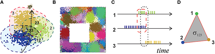
Figure 1. Place fields and place cells. (A) The blue, green, and brown dots, corresponding to the spikes produced by three different place cells, form well-defined spatial clusters, which represent their respective place fields. Spikes are positioned in space according to the animal's coordinates at the time of spiking. (B) A place field map produced by an ensemble of 300 place cells with mean peak firing rate f = 20 Hz and mean place field size s = 14 cm located in a 1 × 1 m environment. (C) A short time segment of the spike trains produced by three place cells. The periods of the cells' coactivity, marked by dashed lines, indicate overlap of their respective place fields (A): cells c₁ and c₂ are coactive in the region 12, cells c₁, c₂, and c₃ are co-active in the region 123. (D) A simplex σ₁₂₃ represents schematically the spatial connectivity encoded by the coactivity of cells c₁, c₂, and c₃. Its 1D edges correspond to pairwise coactivity, e.g., σ₁₂ represents the coactivity of cells c₁ and c₂.

Experimental studies point out that the hippocampal map is topological in nature, i.e., it is more similar to a subway map than to a topographical city map (Gothard et al., 1996; Leutgeb et al., 2005; Alvernhe et al., 2012; Dabaghian et al., 2014). This “topological” hypothesis has a major practical implication: it suggests that hippocampal data should be amenable to topological analyses, thereby allowing us to use powerful arsenals of computational topology. For example, the way place fields cover an environment calls to mind the Alexandrov-Čech theorem that holds that if a space X is covered with a sufficient number of discrete regions, then it is possible to reconstruct topology of X from the pattern of the overlaps between these regions. The argument is based on building a special simplicial complex ${N}$—the nerve of the cover—each n-dimensional simplex of which corresponds to a nonempty overlap of n+1 covering regions, and demonstrating that the topological signatures of ${N}$ and X are same [for details see (Hatcher, 2002) and Methods in (Dabaghian et al., 2012)]. Since, the place cells' spiking activity induces a covering of the environment by the place fields, called a place field map [see Figure 1B and (Babichev et al., 2016)], the Alexandrov-Čech's theorem suggests that the place cells' coactivity (Figure 1C), which marks the overlaps of the place fields, may be used by the brain to represent the topology of the environment. The individual groups of coactive place cells, just like simplices, provide local information about the space, but together, as a neuronal ensemble, they represent space as whole—as the simplicial complex. This analogy establishes a possible approach to the long-sought connection between the cellular and system-scales, which was developed in (Dabaghian et al., 2012; Arai et al., 2014) into a working model of spatial memory. First, it was demonstrated that place cell coactivity can in fact be used to construct a temporal analog of the nerve complex, ${T}$, the simplexes of which, σ = [c₁, c₂, …, c_k], correspond to the combinations of coactive place cells, c₁, c₂, …, c_k (Figure 1D). Second, using the methods of persistent homology (Zomorodian, 2005; Ghrist, 2008) it was shown that the topological structure of ${T}$ captures the topological properties of the environment, if the range of place cell spiking rates and place field sizes happen to parallel biological values derived from animal experiments. Lastly, the persistent homology theory was used to estimate the rate of accumulation of global topological information, i.e., spatial learning.

However, it remained unclear whether it is possible to implement this algorithm in the (para)hippocampal network. On the one hand, electrophysiological studies suggest that place cells showing repetitive coactivity tend to form cell assemblies—functionally interconnected neuronal groups that synaptically drive a readout neuron in the downstream networks (Harris et al., 2003; Harris, 2005; Buzsaki, 2010; Huyck and Passmore, 2013)—which may be viewed as “physiological simplexes” implementing ${T}$. On the other hand, the place cell combinations of ${T}$ are much too numerous to be implemented physiologically. In a small environment, c.a. 1 × 1 m, thousands of place cells are active and the activity of 50–300 of them is near maximal level at every given location (Buzsaki, 2010). The number of combinations of hundreds of coactive cells in an ensemble of thousands is unrealistically large, comparable to $C_{3000}^{100}~10^{200}$. The number of cells in most parahippocampal regions, which may potentially serve as readout neurons, is similar to the number of place cells (Shepherd, 2004). This implies that only a small fraction of coactive place cell groups may be equipped with readout neurons, i.e., that the cell assemblies may encode only a small part of the place cell coactivities—those which represent a “critical mass” of spatial connections.

It is believed that place cells form as a result of competitive learning of inputs provided by the grid cells in the medial entorhinal cortex (MEC), which suggests a particular organization of functional connections between the grid cells and the place cells (Rolls et al., 2006; Solstad et al., 2006). Physiologically, the synaptic architecture of the place cell assembly network (which includes the readout networks downstream from the hippocampus) should also emerge from dynamically changing constellations of synaptic connections, which are commonly studied in terms of the synaptic and structural plasticity mechanisms (Chklovskii et al., 2004; Ghalib and Huyck, 2007; Wennekers and Palm, 2009; Itskov et al., 2011; Caroni et al., 2012). For a better understanding of the qualitative properties of the cell assembly network we propose a biologically plausible phenomenological approach that allows selecting the most prominent combinations of coactive place cells directly and demonstrate that the resulting population of cell assemblies is sufficient for representing the topology of the environment.

We proceed as follows: we start by outlining our methods and formulating general requirements to the model. Then we test three approaches to building a cell assembly network. First, we demonstrate that a “naïve” selection of the cell groups that show repetitive coactivity fails to produce a working cell assembly network. Then we propose two alternative methods of constructing the cell assembly network that reliably capture the topology of the environment. General implications of the approach and possible physiological connections are outlined in the Discussion.

2. The Methods

Mathematically, the task of identifying a subpopulation of coactive place cell combinations corresponds to selecting according to biologically motivated criteria a subcomplex ${T}$₀ of the full coactivity complex ${T}$. The cell assemblies correspond to the maximal simplexes of ${T}$₀, (i.e., the ones that are not subsimplexes of any other simplex), in contrast with the maximal simplexes of the coactivity complex, ${T}$, which can represent any largest combinations of coactive cells. The “cell assembly complex,” ${T}$₀, should satisfy several general requirements:

I. Effectiveness. In the readercentric approach (Buzsaki, 2010), each cell assembly drives a coincidence detector readout neuron in the downstream brain regions. Since the number of the readout neurons is comparable to the number of place cells, the total number of the maximal simplexes in ${T}$₀, N_max(${T}$₀), should be comparable to the number of its vertexes, N_c(${T}$₀),

$N_{\text{max}}({{T}}_0)\approx N_c({{T}}_0).$

However, the algorithm for selecting ${T}$₀ should reduce only the number of coactive place cell combinations and not the place cells themselves, meaning that the number of vertexes in ${T}$ and in ${T}$₀ should not differ significantly. In mathematical literature, the number of k-dimensional simplexes of a simplicial complex is usually denoted as f_k, and the list f = (f₀, f₁, …, f_d) is referred to as the complex's f-vector (Gromov, 1968). However, since in neuroscience literature the letter f is often used to denote firing rates, we denote the number of k-dimensional simplexes by N_k. As a shorthand notation, we use N_max to denote the number of the maximal simplexes and N_c the number of 0-dimensional simplexes in a given complex.

II. Parsimony. To avoid redundancy, only a few cell assemblies should be active at a given location. Conversely, the rat's movements should not go unnoticed by the hippocampal network, i.e., the periods during which all place cell assemblies are inactive should be short.

III. Contiguity. A transition of the spiking activity from one cell assembly σ_i to another σ_i+1 occurs when some cells in σ_i shut off and a new group of cells activates in σ_i+1 (see Supplementary Movies). The larger is the subassembly σ_{i, i+1} = σ_i∩σ_i+1 that remains active during this transition (i.e., the more cells are shared by σ_i and σ_i+1) the more contiguous is the representation of the rat's moves and hence of the space in which it moves. The overlap between a pair of consecutively active simplexes can be characterized by a contiguity index

$\xi =\frac{dim({\sigma }_i\cap {\sigma }_{i+1})}{\sqrt{dim({\sigma }_i)dim({\sigma }_{i+1})}},$

which assumes the maximal value ξ = 1 for coinciding cell assemblies and ξ = 0 for disjoint ones. In constructing a cell assembly complex, we expect that the mean contiguity over the simplexes in ${T}$₀ should not be lower than in ${T}$.

IV. Completeness. The cell assembly complex ${T}$₀ should capture the correct topological signatures of the environment, such as obstacles, holes, and boundaries. For example, the lowest dimensional 0D and 1D loops in ${T}$₀ represent, respectively, the piecewise and the path connectivity of the environment, as they are captured by the place cell coactivity. This information should emerge from the “topological noise” in a biologically plausible time period, comparable to the time required to obtain this information via the full complex, ${T}$ [see (Dabaghian et al., 2012; Arai et al., 2014) and Figure 2].

FIGURE 2

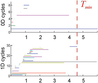
Figure 2. Topological loops: each horizontal bar represents the timeline of a topological cycle in ${T}$(T): 0D loops (connectivity components) and the 1D loops. Most cycles last over a short time before disappearing. A few remaining, persistent loops express stable topological information that may correspond to physical obstacles in the rat's environment. The time required for the correct number of cycles to appear is interpreted as the minimal time T_min required for the rat to learn the environment. The environment used in these simulations (Figure 1B) is topologically connected (b₀ = 1), and has one central hole (b₁ = 1), and no topological signatures in higher dimensions (b_n>1 = 0). Thus, the topological barcode of this environment—the list of Betti numbers (b₀, b₁, b₂,…)—is (1,1, 0, …). The last spurious loop (blue 1D timeline on the bottom panel) disappears at about T_min = 4.6 min, which is the learning time in this case.

2.1. Place Cell Spiking

Place cell spiking is modeled as a time-dependent Poisson process with spatially localized rate

${\lambda }_c(r)=f_c{e}^{-\frac{{(r-r_c)}^2}{s_c^2}},$

where r is a point in the environment, f_c is the maximal firing rate of a place cell c, and s_c defines the size of the corresponding place field centered at r_c (Barbieri et al., 2004). In a familiar environment, the place fields are stable, that is, the parameters f_c, s_c, and r_c remain constant (Wilson and McNaughton, 1993; Brown et al., 2001). In our simulations, all computations were performed for 10 place cell ensembles, each containing 300 neurons with an ensemble mean maximal firing rate of 20 Hz and a mean place field size of 30 cm. The place field centers in each ensemble were randomly scattered across the environment and most quantities reported in the Results were averaged over ten place field configurations.

2.2. Spatial Map

We simulated the rat's movements through a small (1 × 1 m) planar environment (Figure 1B), similar to the arenas used in typical electrophysiological experiments [see Methods in (Dabaghian et al., 2012)] over T = 25 min—the duration of a typical “running session.” The spatial occupancy rate of the rat's trajectory (i.e., the histogram of times spent at a particular location) and the frequency of the place cells' activity are shown on Figures 3A,B. The mean speed of the rat is 20 cm/sec, so that turning around the central obstacle takes about 7 s.

FIGURE 3

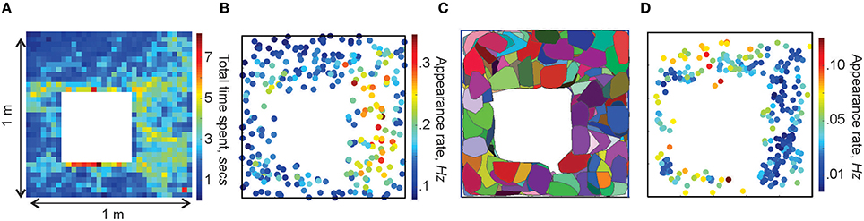
Figure 3. Spatial maps. (A) Occupancy of spatial locations in a 1 × 1 m environment—a 2D histogram of the time spent by the animal in different locations. (B) Frequency of place cells' spiking: each dot marks the location of a place cell's center r_c and indicates the corresponding appearance rate according to the colorbar. Higher appearance rates appear in the domain where the spatial occupancy is higher. (C) Simplex field map. The place field map for the same place cell ensemble is shown in Figure 1B. (D) Spatial distribution of the frequency of the maximal simplexes' appearances. Notice that, since place cells with higher appearance rates tend to produce higher order cell assemblies, which, in turn, have lower appearance rates, the spatial distribution of rates on (B,D) are complementary.

By analogy with the place fields, we designate the spatial domain where a combination of place cells comprising a simplex σ is active as its simplex field, s_σ (Figure 3C). If the simplex corresponds to a cell assembly, then s_σ may also be referred to as the cell assembly field. Similarly to the place fields and the place field map (Figure 1B), the collection of all simplex fields forms a simplex field map and the cell assembly fields form a cell assembly map (Figure 3C). These maps provide a better “geometric proxy” for the rat's cognitive map because they illustrate both the activity and the coactivity of the individual place cells (Figures 3C,D). In the following, the structure of these maps will be used to discuss our selection algorithms. If the distinction between a cell assembly map and a simplex map is not essential, it will be referred to as a space map.

2.3. Population Activity

To define the population code (Pouget et al., 2000) of place cell combinations, we construct place cell activity vectors by binning spike trains into w = 1∕4 s long time bins [for a physiological justification of this value see (Mizuseki et al., 2009; Arai et al., 2014)]. If the time interval T splits into n such bins, then the activity vector of a cell c is

$m_c(T)=\left[m_{c,1},\dots ,m_{c,n}\right],$

where m_{c, k} specifies how many spikes were fired by c in the k^th time bin. The components of m_c, normalized by the total number of spikes, M_c, define spiking probabilities, p_{c, k} = m_k∕M_c (Perkel et al., 1967). A stack of activity vectors forms an activity raster illustrated on Figure 4.

FIGURE 4

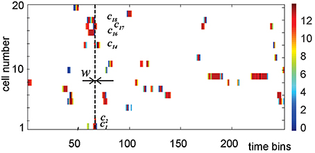
Figure 4. An activity raster of a population of 20 place cells over 250 time bins. Each row defines the activity vector of the corresponding place cell. The color of the ticks indicates the number of spikes contained in the corresponding bin of width w, according to the colorbar on the right. At every time step, the nonempty bins in the vertical column define the list of currently active cells, i.e., the active simplex σ_t. During the time interval marked by the vertical dashed line, cell c₁, c₂, c₁₄, c₁₆, c₁₇, and c₁₈ are coactive, producing the coactivity simplex of fifth order σ = [c₁, c₂, c₁₄, c₁₆, c₁₇, c₁₈].

Two cells, c₁ and c₂, are coactive over a certain time period T, if the dot product of their activity vectors does not vanish,

$m_{c_1}(T)·m_{c_2}(T)\ne 0.$

The component-wise or Hadamard product of two activity vectors

$m_{c_1,c_2}=m_{c_1}\odot m_{c_2}=\left[m_{c_1,1}{m}_{c_2,1},m_{c_1,2}{m}_{c_2,2},\dots ,m_{c_1,n}{m}_{c_2,n}\right]$

defines the coactivity vector of cells c₁ and c₂, which can also be viewed as the activity vector of the corresponding 1D simplex σ₁₂ = [c₁, c₂], m_σ12 ≡ m_{c1, c2}. Similarly, the Hadamard product of k vectors,

$\begin{array}{l}{m}_{{\sigma }_{12\dots k}}=m_{c_1,c_2,\dots ,c_k}=m_{c_1}\odot m_{c_2}\odot \dots \odot m_{c_k},\end{array}$

defines the activity vector of the simplex σ_12…k = [c₁, c₂, …, c_k].

For each activity vector, m_σ, we also define its bit array mapping into a binary appearance vector, a_σ, which indicates during which time-bins the corresponding simplex σ has made its appearance, i.e., a_{σ, i} = 1 iff m_{σ, i} > 0. The appearance rate, f_σ(T), of a simplex σ over a time interval T, is defined as the L₁ norm of its appearance vector, averaged over that time interval,

$f_{\sigma }(T)=(1∕T){\Sigma }_i{a}_{\sigma ,i}.$

These appearance vectors and appearance rates allow distinguishing the intrinsic physiological characteristics of place cells' spiking, e.g., their maximal firing rate, from the frequency with which these cells activate due to the rat's movements through their respective place fields. While the maximal firing rate of a typical place cell is about 15 Hz (Best et al., 2001), the frequency of their activation is much lower.

3. Results

The simulated ensembles of 300 place cells in the environment shown on Figure 1B produced a coactivity complex ${T}$ with about N_max = 1000 maximal simplexes. Despite the high dimensionality of these simplexes (up to D = 35, mean $\stackrel{-}{D}=17$), the characteristic dimensionality of a facet shared by two consecutively active simplexes, σ_i and σ_i+1, is relatively low, so that the mean contiguity of ${T}$ is ξ = 0.6. This implies that, geometrically, if the simplexes of ${T}$ are viewed as multidimensional tetrahedrons, the selected complex, ${T}$₀(θ), assumes a highly irregular shape (Supplementary Figure 1A).

More importantly, nearly 100% of the maximal simplexes appeared only once during the entire 25 min period of navigation, i.e., a typical maximal simplex's appearance rate is low, $f_{\sigma }~10^{-3}$ Hz. However, a typical vertex activated about 200 times or every seven seconds, suggesting that some of the lower dimensional subsimplexes may be better candidates for forming cell assemblies. Is it then possible to build a cell assembly complex ${T}$₀ by discarding the high-dimensional maximal simplexes with low appearance rates and retaining their subsimplexes that appear more frequently? We tested this hypothesis by identifying the combinations σ whose coactivity exceeds a certain threshold f_σ > θ, and studied the properties of the resulting simplicial complex as a function of θ (Figure 5A).

FIGURE 5

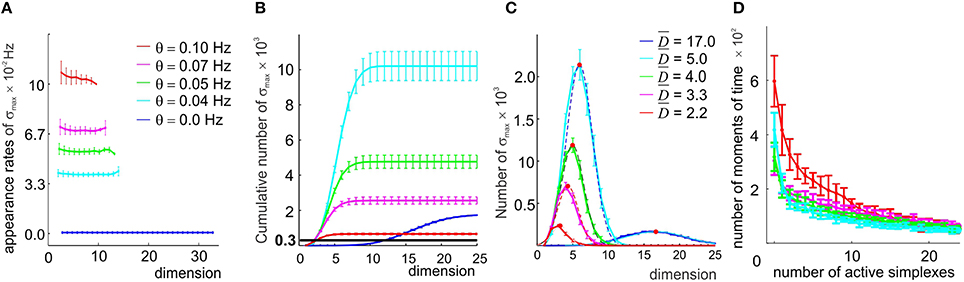
Figure 5. A direct selection of the simplexes by appearance rates. (A) In the original coactivity complex ${T}$(θ = 0), the maximal simplexes σ_max appear on average but once during the entire observation period, resulting in low appearance rates ($f_{\sigma }<10^{-3}$ Hz, blue line). Imposing four different thresholds θ (color coded) raises the appearance rates of the selected maximal simplexes almost uniformly in all dimensionalities. (B) Cumulative distribution of the number of maximal simplexes N_max over the selected simplexes' dimension. In the ${T}$(θ = 0) case N_max exceeds the number of vertexes (N_c = 300, black horizontal line) by almost an order of magnitude. Small threshold values result in an explosive increase of N_max which then begins to decrease for θ > 0.04 Hz, remaining significantly higher than N_c for all four tested values of θ. (C) The histograms of the maximal simplexes' dimensionalities fit with normal distribution. The high mean dimensionality ($\stackrel{-}{D}=17$) observed in the ${T}$(θ = 0) case reduces to $\stackrel{-}{D}=2.2$ for θ = 0.1 Hz. The width of the distributions is about 50% of $\stackrel{-}{D}$. (D) The histograms of the number of the coactive maximal simplexes, fit to an exponential distribution, demonstrate that the typical number of coactive simplexes is large, β > 10. All values are averaged over ten place field maps generated by 10 place cell ensembles with the same mean peak firing rate and mean place field size.

First we observed that, as soon as the appearance threshold is introduced (θ≳10⁻³ Hz), the high dimensional simplexes start breaking up, releasing large numbers of lower dimensional subsimplexes: the number of k-dimensional subsimplexes in a n-dimensional simplex grows as combinatorial coefficient $C_{n+1}^{k+1}$, e.g., for n = 17 and k = 7, $C_{18}^8\approx 44,000$. As a result, the complex ${T}$₀(θ) rapidly inflates. As θ increases further (θ > 0.04), the number of “passing” simplexes decreases, and ${T}$₀(θ) begins to shrink in all dimensions (i.e., N_D(θ₁) > N_D(θ₂) for θ₁ < θ₂, for all D, (Figure 5B). Despite this, the number of maximal simplexes remains high: N_max = 30 × N_c at θ = 0.04 Hz, N_max = 7 × N_c at θ = 0.07 Hz and N_max = 3 × N_c for the highest tested threshold, θ = 0.1 Hz (Figure 5B), while their characteristic dimensionality drops from D = 17 to D = 7 at θ = 0.04 Hz and to D = 3 at θ = 0.1 Hz. The mean contiguity index for this range of thresholds remains close to ξ = 0.7, indicating that the degree of overlap between the selected combinations of place cells is higher than in the original coactivity complex.

However, raising the passing threshold θ quickly destroys the geometric integrity of the resulting complex's spatial map. As shown on Supplementary Figure 2, for θ = 0.05 Hz, only ~50% of the environment is covered by the remaining simplex fields, and for θ = 0.07 Hz the simplex map barely retains its one-piece connectedness: in some cases the complex ${T}$₀ splits in two (the corresponding Betti numbers, b₀, are listed in Supplementary Table 1, for an illustration see Supplementary Figure 3). For θ = 0.1 Hz, the complex fragments into multiple components (mean b₀ ~ 7) that are riddled with holes: the Betti numbers b_n>0 indicate the presence of hundreds of stable loops in higher dimensions. Thus, even if the coactive place cell combinations selected at θ ≥ 0.05 Hz could be supplied with readout neurons and would form cell assemblies, the resulting cell assembly network would not encode the correct spatial connectivity.

An additional problem is that reducing the order of the assemblies violates the “assembly code” for spatial locations: every time several subsimplexes σ_i are selected from a high-order maximal simplex σ, several overlapping simplex fields s_σi are produced in place of a single s_σ. As a result, the parsimony of the representation is compromised: a location that was previously represented by a single simplex becomes represented by a few of its subsimplexes (Supplementary Figures 4A,B). Figure 5D shows a histogram of the numbers of simultaneously active maximal simplexes in ${T}$₀: although most of the time only a few maximal simplexes are active, a coactivity of many of them (n > 25) is not uncommon. Conversely, while most of the time—on average 84% for the selected place cell ensembles—at least one simplex is active, longer inactivity periods are observed as described by double exponential distributed with the rate β ≈ 3.5 s (Supplementary Figure 2).

Overall, since most of the ${T}$₀-requirements listed in the Methods fail, we are led to conclude that the most straightforward selection rule, based on selecting high appearance rates, does not produce the desired tradeoff between the order of the assemblies, the frequency of their appearances, and the quality of topological representation of the environment. This failure motivates the search for alternative methods.

3.1. Method I

To produce a more detailed approach to selecting coactive cell combinations, we observe that place fields are typically convex planar regions, and hence the existence of higher order overlaps between them actually follows from the lower order overlaps. According to Helly's theorem, a collection of n > D+1 convex D-dimensional regions in Euclidean space R^D will necessarily have a nonempty common intersection, if the intersection of every set of D+1 regions is nonempty (see (Eckhoff, 1993; Avis and Houle, 1995) and Supplementary Figure 4D). From the perspective of Čech theory, this implies that if n convex regions which cover a D-dimensional space contribute all the combinatorially possible D-dimensional simplexes to the nerve complex, then they also provide all the higher (up to n − 1) dimensional simplexes to it. In a planar (D = 2) environment, this implies that a set of four or more place fields has a common intersection, if any three of them overlap. Moreover, although mathematically it is possible that three place fields exhibit pairwise, but not triple overlap, the probability of such an occurrence is low (Supplementary Figure 4C). A direct computational verification shows that if a triple of place cells demonstrates pairwise coactivity, then, in over 90% of cases, it also correctly encodes a triple spatial overlap. In other words, a “clique” of pairwise coactivities indicates the overlaps of all higher orders, which implies that the spatial connectivity graph G_${N}$ whose vertexes correspond to the place fields and links represent pairwise overlaps, encodes most simplexes in the nerve complex ${N}$.

As a reminder, a clique of an undirected graph is a set of pairwise connected vertices. From the combinatorial perspective, a clique and a simplex have the same defining property: any subset of a simplex is its subsimplex and any subset of a clique is its subclique; a maximal clique is the one that is contained in no other clique. Hence, each graph defines its own “clique complex,” the k-dimensional simplexes of which corresponds to the graph's cliques with k + 1 vertices (Bandelt and Chepoi, 2008).

The observation that the nerve complex induced from the place field map can be approximated by the clique complex of the place field pairwise connectivity graph, suggests that the corresponding coactivity complex ${T}$ can also be built based only on pairwise, rather than higher-order, coactivities. This approach is well justified physiologically, since pairwise coactivity detector pairs of synapses are commonly observed (Katz et al., 2007; Brette, 2012). The rule for defining the temporal analog of G_${N}$—the relational graph G_${T}$—is straightforward: a pair of vertexes is connected in G_${T}$ if the corresponding cells c_i and c_j are coactive. Thresholding pairwise coactivity rates according to the rule

$\begin{array}{ll}{C}_{ij}=\{\begin{array}{ll}1\hfill & \text{if }{f}_{c_i,c_j}\ge \theta \hfill \\ 0\hfill & \text{if }{f}_{c_i,c_j}<\theta .\hfill \end{array}& (1)\end{array}$

allows constructing a family of relational graphs G_${T}$(θ) over the pairs of place cells with high coactivity. The higher the threshold is, the sparser its connectivity matrix C_ij and the smaller the number of maximal cliques and hence of maximal simplexes in the corresponding clique complex. Since in the following the graph G_${N}$ will not be used we will suppress the subscript “${T}$” in the notation for G_${T}$.

We studied the relational graphs G(θ) and their respective clique complexes ${T}$₀(G(θ)) ≡ ${T}$₀(θ) as a function of θ. First, we observed that the appearance rates of the maximal simplexes in ${T}$₀(θ) become sensitive to the simplexes' dimensionality (Figure 6A), implying that this selection procedure in effect attributes different thresholds to simplexes of different dimensions by using only one free parameter θ. Second, the size of ${T}$₀(θ) is not as large as before. As shown on Figures 6B–D, even for a relatively low threshold θ = 0.05 Hz, the number of maximal simplexes exceeds the number of cells only marginally. For higher thresholds, this number steadily decreases: N_D(θ₁) < N_D(θ₂) for θ₁ > θ₂ > 0.04 and D > 3, though in lower dimensions (1 ≤ D ≤ 3) this number may increase. The characteristic contiguity ranges between ξ = 0.65 at θ = 0.05 Hz to ξ = 0.72 at θ = 0.14 Hz, which is higher than the value produced by the direct simplex selection method. Geometrically, this implies that the collection of maximal simplexes selected by pairwise threshold selection is more aggregated than the collection produced via direct simplex selection, i.e., the resulting complex ${T}$₀(θ) is geometrically more similar to a “simplicial quasimanifold” (see Supplementary Figure 1B). However, the number of place cells N_c drops as a result of discarding too many links with low appearance rate: N_c = 290 at θ = 0.05 Hz and N_c = 100 at θ = 0.14 Hz. At θ = 0.1 Hz number of cells levels out with the number of maximal simplexes, N_max ~ N_c = 260.

FIGURE 6

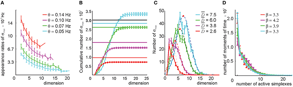
Figure 6. Selecting maximal simplexes via the pairwise coactivity threshold (Method I). (A) The appearance rates of the maximal simplexes computed for four different pairwise appearance rate thresholds θ decrease as a function of their dimensionality. The values at D = 1 correspond to the value of the threshold imposed on the links' appearance rate. (B) Cumulative distribution of the numbers of maximal simplexes, N_max, over the selected simplexes' dimension. The numbers of cells N_c for each threshold value are shown by horizontal lines. The tendency of the maximal simplexes to outnumber the vertexes N_max > N_c, characteristic for small values of θ, is reversed around θ = 0.07 Hz, where N_max and N_c level out. (C) The histograms of the maximal simplexes' dimensionalities fit with normal distribution. The mean dimensionalities are similar to the ones produced by the previous selection method. The width of the distributions is about 50% of $\stackrel{-}{D}$. (D) The histogram of the number of coactive maximal simplexes, fit to an exponential distribution, shows that the expected number of coactive simplexes (β ~ 4) is significantly lower than in the previous selection method. The procedure of averaging over the place field maps is the same.

As before, raising the coactivity threshold degrades the spatial map. At θ > 0.07 Hz the simplex fields no longer cover the environment and at θ > 0.1 Hz the map fragments into pieces (Supplementary Figure 5). However, the resulting complex exhibits a much more regular topological behavior: the correct signature (b₀ = 1, b₁ = 1, b₂ = 0, b₃ = 0, …) in ${T}$₀(θ) appears at θ = 0.05 Hz. The higher order Betti numbers (b_n≥2) remain trivial at still higher θs (Supplementary Table 2A), even though the connectedness and path connectivity of the environment (b₁ and b₀) become misrepresented.

This improvement of the behavior of ${T}$₀(θ) suggests that, despite all the shortcomings, the link-selection strategy may lead to a successful model of the place cell assembly network. After all, it is not surprising that a single selection rule does not resolve all the aspects of the cell assembly formation. Yet if it captures the essence of the process, it should be possible to correct or to adjust its outcome. For example, one of the difficulties faced by the coactivity selection algorithm is that, for high θ, ${T}$₀(θ) may brake into several pieces. However, the gaps between them are small. Thus, if a few discarded edges of the relational graph that originally bridged these gaps are retained, then the connectedness of ${T}$₀(θ) may be spared (Figure 7A). Similarly, a “hole” in the relational graph is a linear chain of edges, connected tail to tail, with no shortcuts. However, if the links with the lower appearance rate (f ≥ θ_h, θ_h < θ) that span across the hole exist at θ = 0, then they also can be restored (Figure 7B). This may remove the non-contractible chains of 1D simplexes in ${T}$₀(θ) that compromised its path connectivity (Figures 7C,D). Thus, we implemented the following two rectification algorithms:

1. Filling gaps: find pairs of vertexes v_a and v_b separated in G(θ) by more than n_g edges and then test whether these vertexes are connected directly by links (from G(θ = 0)) whose appearance rate exceeds a lower threshold θ_g < θ. If such links exist, add them to G(θ) (red lines on Figure 7C).

2. Closing holes: A closed chain containing m_h ≥ 4 edges in G(θ), with no shortcuts, is likely to produce a hole in ${T}$₀(θ). We identified such chains and restored the discarded cross-links whose appearance rate exceeds a lower threshold θ_h < θ.

FIGURE 7

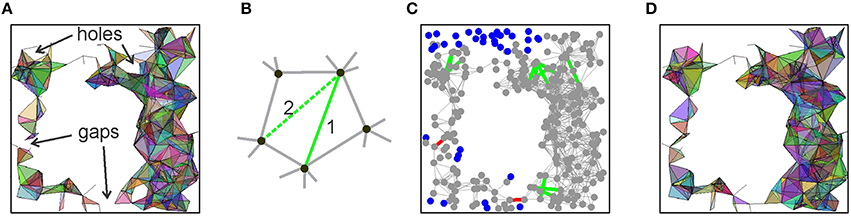
Figure 7. Correction algorithms. (A) A spatial projection of the 2D skeleton of ${T}$(θ) shows gaps and holes that compromise, respectively, the piecewise and path connectivity of ${T}$(θ). If the links across the gaps and holes of ${T}$(θ) are restored, then its correct connectivity structure may be regained. (B) A “hole” produced by five connected vertexes is closed by restoring some of the previously discarded crosslinks. (C) A projection of the relational graph G into the environment, shown in gray. The edges added across the gaps are shown in red and the edges added to fill the holes are shown in green. The vertexes that are left disconnected due to low appearance rates of the edges connecting them to other vertexes are shown by blue dots. (D) A spatial map of the resulting “patched” 2D skeleton of ${T}$(θ). The parameter values are n_g = 15, m_h = 10, and the lowered threshold for reintroducing the missing links is θ = 50.

Thus, both rectification algorithms depend on two parameters: the length of the involved chains (n_g for gaps and m_h for holes) and the value of the reduced threshold θ_g and θ_h. In our numerical experiments, we found that the optimal value for the thresholds is θ_h = θ_g = 50, and the parameters range between 5 and 10 (m_h) and 10 and 15 (n_g). Typically, each rectification procedure is applied once or twice before the right signature of ${T}$₀(θ) is achieved, and this without producing significant changes of the complex's structure, such as altering the appearance of its simplexes or increasing its size N_max. As illustrated in the Supplementary Table 2B, the correct signature in the “repaired” complex is achieved for all cases at θ = 0.07 Hz. In particular, at θ = 0.07 Hz we obtain a simplicial complex ${T}$₀ with the correct signature, having N_c = 260 vertexes and about the same number of maximal simplexes, N_max ≈ N_c. These maximal simplexes appear on average at a rate of f_σ ≥ 0.07 Hz, at least during every other run of the rat around the environment, and have dimensionality D = 6. As a result, the requirements to ${T}$₀ are met and the maximal simplexes of ${T}$₀ may represent hippocampal place cell assemblies that together encode a map of the environment, and hence ${T}$₀ itself can be viewed as the “cell assembly complex.”

3.2. Method II

A common feature of the appearance-rate-based selection rules is that the resulting simplicial complex reflects biases of its spatial occupancy: higher dimensional maximal simplexes concentrate over the parts of the environment where the rat appears more frequently. In particular, the relational graph shows a higher concentration of edges over the eastern segment of the environment (Figure 7C) where the occupancy rate is highest (Figure 3A). On the one hand, this is natural since the frequency of the place cells' spiking activity certainly does depend on the frequency of the rat's visits to their respective place fields, which therefore affects the hippocampal network's architecture (Chklovskii et al., 2004; Caroni et al., 2012). In fact, this argument is at the core of the classical “hippocampus as a cognitive graph” model (Burgess and O'Keefe, 1996; Muller et al., 1996), which proposes that the architecture of the hippocampal network is an epiphenomenon of the place cell coactivity. On the other hand, the physiological processes that produce synaptic connections may be more autonomous. For example, the CA3 region of the hippocampus is anatomically a recurrent network of place cells whose spiking activity and synaptic architecture are dominated by the network's attractor dynamics (Tsodyks, 2005; Wills et al., 2005; Colgin et al., 2010).

These considerations lead us to test an alternative method of constructing the relational graph based on selecting, for every cell, its n₀ closest neighbors as defined by the pairwise coactivity rate f_{ci, cj}. Note that the resulting number of connections may be different for different cells: a cell c₁ may be among the n₀ closest neighbors of a cell c₂, and hence c₁ and c₂ become connected, but the set of n₀ closest neighbors of a cell c₁ may not include c₂, which bears a certain resemblance to the preferential attachment models (Barabasi and Albert, 1999). As a result, the vertex degrees k of the (undirected) relational graph may differ from one another and from n₀. A direct computational verification shows that k is distributed according to a power law, P(k) ~ k^−γ, where γ ranges, for different n₀, between γ ~ 2 and γ ~ 4 (Figure 8), which implies that G(n₀) demonstrates scale-free properties (Barabasi and Albert, 1999; Albert and Barabasi, 2002) characteristic of the hippocampal network (Bonifazi et al., 2009; Li et al., 2010). In contrast, the histogram of the vertex degrees in the threshold-controlled relational graph G(θ) may be fit with the negative binomial distribution (Figure 8B), which indicates that G(θ) is similar to a random graph.

FIGURE 8

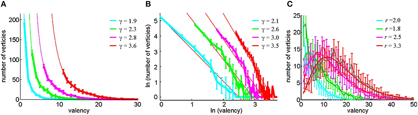
Figure 8. Statistics of the vertex degrees in relational graphs. (A) The histogram of the vertex degrees k in the neighbor-controlled relational graph G(n₀), computed for n₀ = 2, 4, 7, 12 (Method II) and fitted to a power law distribution P(k) ~ k^−γ. The graph demonstrates that G(n₀) is a scale-free network. (B) The same distribution on the log-log scale and an independent linear fit of the powers γ. The confidence intervals of the two fits, ranging between ±0.15 and ±0.3, overlap for each case. (C) In the pairwise coactivity threshold (Method I), the histogram of the relational graph's vertex degrees is fit by negative binomial distribution, suggesting that G(θ) is similar to a random network.

This neighbor-selection method for building the relational graph G(n₀) has a number of other immediate advantages over the threshold-controlled construction of G(θ). For example, no cells are excluded from ${T}$₀ due to the low appearance of the edges connecting to them. As a result, the simplex fields are distributed more uniformly (Supplementary Figure 6), which helps capture the correct piecewise connectedness of the environment.

By studying the properties of the clique complexes produced by the relational graphs G(n₀) for n₀ = 2, 4, 7, and 12—parameters chosen to produce similar numbers of edges as in the previous method—we found that the number of maximal cliques in ${T}$₀(G(n₀)) is typically lower than in ${T}$₀(G(θ)). The appearance rates of maximal cliques in G(n₀) are more scattered and less sensitive to dimensionality than in G(θ) (Figure 9A and Supplementary Figure 6). The number of maximal simplexes in ${T}$₀(n₀) remains close to the number of cells (Figures 9B,D) and their dimensionality is lower than in the threshold-based selection approach (Figure 9C). The contiguity index in all complexes ranges between to ξ = 0.67 and ξ = 0.71. The coverage of the space with the simplex fields improves with growing n₀ (see Supplementary Figure 6)—for n₀ > 2 the complex ${T}$₀(n₀) is connected, while the behavior of b₀ is more regular (see Supplementary Table 3). However, the path connectivity of the complex ${T}$₀(n₀) remains deficient for all n₀ because the number of stable spurious 1D loops remains high (Supplementary Table 3). After filling the gaps and closing the holes, most complexes constructed for n₀ ≥ 7 acquire correct topological signatures (Supplementary Table 3), and the requirements to ${T}$₀ are satisfied. Thus, the simplicial complex obtained by the neighbor selection method for n₀ ≥ 7 can also be viewed as a “cell assembly complex,” meaning it can serve as a formal model of the place cell assembly network with mean contiguity ξ = 0.7.

FIGURE 9

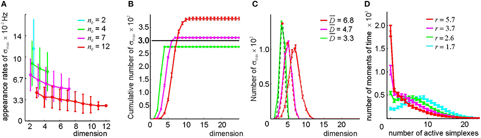
Figure 9. Selecting maximal simplexes via best neighbor selection (Method II). (A) The appearance rates of the maximal simplexes in the simplicial complex ${T}$(n₀), computed for four different values of n₀ (color coded), decrease as a function of their dimensionality. (B) Cumulative distribution of the number of maximal simplexes N_max over the selected simplexes' dimension. For the tested values of n₀, the fixed number of vertexes N_c = 300, indicated by the horizontal black line, is close to the number of maximal simplexes. For n₀ = 7, the values N_max and N_c come closest. (C) The histograms of the maximal simplexes' dimensionalities, fit to the normal distribution, indicate that for the relational graph with a similar number of links, the mean dimensionalities of the maximal simplexes are smaller than in in the complex built via the threshold-selection method. The width of the distributions is about 40% of $\stackrel{-}{D}$. (D) The histogram of the number of coactive maximal simplexes, fit to a gamma distribution. An expected number of coactive simplexes ranges between r = 2 and r = 6. The procedure of averaging over the place field maps is the same.

4. Discussion

The hippocampal representations of the environment are based on the temporal organization of the place cells' spiking and on the mechanisms of processing the resulting spike trains in the downstream networks. While the place cells' spiking determinants [both spatial (O'Keefe and Burgess, 1996; Jeffery et al., 1997; Fenton et al., 2000) and nonspatial (Sharp et al., 1995; Wood et al., 2000)] are relatively well–studied, the readout mechanisms remain poorly understood. It is believed that groups of place cells exhibiting frequent coactivity form assemblies that jointly trigger spiking activity of their respective readout neurons, but the specific architecture of the cell assembly network has not been fully identified.

4.1. Descriptive vs. Phenomenological Approach

Previously, the topological approach was used to quantify the information encoded by the hippocampal network. Each individual group of coactive place cells, contributing local information about the space, was represented by a simplex, and hence the entire neuronal ensemble, encoding space as whole, was represented by a coactivity complex ${T}$ (Curto and Itskov, 2008; Dabaghian et al., 2012; Arai et al., 2014). Specifically, the low order (pair and triple) coactivity events were used to construct the 2D skeleton of ${T}$, and then its 0D and 1D topological loops were matched with the topological loops in the environment. In the current work, the topological approach is extended to produce the functional architecture of the cell assembly network—schematically represented by a cell assembly complex ${T}$₀—and relating its structure to the net topological information it encodes. In contrast with ${T}$, the maximal simplexes of ${T}$₀ are viewed as representations of the physiological place cell assemblies, rather than any largest combinations of the coactive place cell groups. In particular, the model allows constructing the higher order assemblies that may potentially represent both the low-dimensional spatial environment and the high-dimensional memory space (Eichenbaum et al., 1999; Buzsaki, 2010). Importantly, the learning times T_min estimated from the dynamics of the 0D and 1D loops in ${T}$₀ remain close to the learning times computed for the full coactivity complex ${T}$ (see Supplementary Table 4). This implies that the selected, “core” pool of coactive place cell combinations captures the topological structure of the environment as fast and as reliably as the entire set of the place cell coactivities.

4.2. Physiological Connections

In order to elicit an action potential, the impinging spikes must conjointly hyperpotentiate the readout neuron. A qualitative insight into this process was suggested by (Jarsky et al., 2005), who demonstrated that a pair of impinging synapses can “gate” one another: if a synaptic input s₂ comes within a short period w after the synaptic input s₁, then together these two inputs can polarize a large segment of the dendritic tree, which may lead to hyperpolarization of the entire postsynaptic neuron. This mechanism can be viewed as a physiological implementation of the “coincidence detection” for a pair of inputs and one can immediately see how it could be used to detect a larger (k > 2) number of inputs. One can think of the k nearly-simultaneous individual inputs s_i as of k(k − 1)∕2 nearly-simultaneous pairs of inputs (s_i,s_j), each one of which polarizes a particular fragment d_ij of the dendritic tree. If the physiology of the readout neuron is such that it hyperpotentiates only in response to nearly simultaneous inputs (s_i,s_j), then the readout neuron functions as a coincidence detector. In contrast, if the dendritic tree can retain the local polarizations over an extended period ϖ > w, then such neuron will integrate low order inputs over that time.

The links in the coactivity graph ${G}$ can be viewed as schematic representations of the pairs of potentiating synapses: the proposed Methods I and II represent two possible ways of selecting the most “prominent” pairs. In Method I, the “winning pairs” of mutually gating synapses are selected based on the frequency of their appearance. Alternatively, given the number n₀ of connections that a given cell can produce (based, e.g., on the number of axon terminals), one can aim to select these connections optimally—this is Method II.

4.3. Developments

We view the proposed algorithms as basic models of a general “phenomenological” approach that can be further developed along several broad lines. First, the structure of the relational graph is currently deduced from the activity vectors defined over the entire navigation period T = 25 min. A biologically more plausible selection algorithm should be adaptive: the structure of the relational graph at a given moment of time t < T should be based only on the spiking information produced before t. Hence, in a more advanced model, the structure of the relational graph should develop in time, and in general the cell assemblies comprising ${T}$₀ should be derived using synaptic and structural plasticity mechanisms. Second, the selection criteria in Methods I and II above may be individualized: the appearance threshold used to construct the relational graph can be assembly-specific, i.e., θ = θ(σ), so that the properties of the resulting network would be described in terms of the probability distribution of the threshold values across the cell assembly population. Similarly, the number of neighbors can be made cell-specific, n₀ = n₀(c_i), which should permit better control over the topological properties both of the network and of the cell assembly complex. Third, threshold control can be implemented using different coactivity metrics, for instance via the pairwise correlation coefficient

$\begin{array}{ll}\rho (c_1,c_2)=(m_1·m_2)∕\left|m_1\right|\left|m_2\right|,& (2)\end{array}$

which would connect cells with correlated spiking (irrespective of their firing rates), in contrast with the metric (2), which does the opposite. In general, two metrics ρ and ρ′, produce relational graphs with different topologies. Nevertheless, they may produce similar or identical large-scale effects, such as generating topologically identical cell assembly complexes ${T}$₀, or exhibit similar learning times, T_min. Identifying classes of metrics that produce topologically similar results will be examined in future research.

Author Contributions

All authors listed, have made substantial, direct and intellectual contribution to the work, and approved it for publication.

Funding

The work was supported in part by Houston Bioinformatics Endowment Fund, the W. M. Keck Foundation grant for pioneering research and by the NSF 1422438 grant.

Conflict of Interest Statement

The authors declare that the research was conducted in the absence of any commercial or financial relationships that could be construed as a potential conflict of interest.

Acknowledgments

I thank R. Phenix for his critical reading of the manuscript.

Supplementary Material

The Supplementary Material for this article can be found online at: https://www.frontiersin.org/article/10.3389/fncom.2016.00050

References

Albert, R., and Barabasi, A.-L. (2002). Statistical mechanics of complex networks. Rev. Modern Phys. 74, 47–97. doi: 10.1103/RevModPhys.74.47

CrossRef Full Text | Google Scholar

Alvernhe, A., Sargolini, F., and Poucet, B. (2012). Rats build and update topological representations through exploration. Anim. Cogn. 15, 359–368. doi: 10.1007/s10071-011-0460-z

PubMed Abstract | CrossRef Full Text | Google Scholar

Arai, M., Brandt, V., and Dabaghian, Y. (2014). The effects of theta precession on spatial learning and simplicial complex dynamics in a topological model of the hippocampal spatial map. PLoS Comput. Biol. 10:e1003651. doi: 10.1371/journal.pcbi.1003651

PubMed Abstract | CrossRef Full Text | Google Scholar

Avis, D., and Houle, M. E. (1995). Computational aspects of Helly's theorem and its relatives. Int. J. Comput. Geometry Appl. 05, 357–367. doi: 10.1142/S0218195995000222

CrossRef Full Text | Google Scholar

Babichev, A., Cheng, S., and Dabaghian, Y. A. (2016). Topological schemas of cognitive maps and spatial learning. Front. Comput. Neurosci. 10:18. doi: 10.3389/fncom.2016.00018

PubMed Abstract | CrossRef Full Text | Google Scholar

Bandelt, H. J., and Chepoi, V. (2008). Metric graph theory and geometry: a survey. Contemporary Math. 453, 49–86. doi: 10.1090/conm/453/08795

CrossRef Full Text | Google Scholar

Barabasi, A.-L., and Albert, R. (1999). Emergence of scaling in random networks. Science 286, 509–512.

PubMed Abstract | Google Scholar

Barbieri, R., Frank, L. M., Nguyen, D. P., Quirk, M. C., Solo, V., Wilson, M. A., et al. (2004). Dynamic analyses of information encoding in neural ensembles. Neural Comput. 16, 277–307. doi: 10.1162/089976604322742038

PubMed Abstract | CrossRef Full Text | Google Scholar

Best, P. J., and White, A. M. (1998). Hippocampal cellular activity: a brief history of space. Proc. Natl Acad. Sci. U.S.A. 95, 2717–2719.

PubMed Abstract

Best, P. J., White, A. M., and Minai, A. (2001). Spatial processing in the brain: the activity of hippocampal place cells. Ann. Rev. Neurosci. 24, 459–486. doi: 10.1146/annurev.neuro.24.1.459

PubMed Abstract | CrossRef Full Text | Google Scholar

Bonifazi, P., Goldin, M., Picardo, M. A., Jorquera, I., Cattani, A., Bianconi, G., et al. (2009). GABAergic hub neurons orchestrate synchrony in developing hippocampal networks. Science 326, 1419–1424. doi: 10.1126/science.1175509

PubMed Abstract | CrossRef Full Text | Google Scholar

Brette, R. (2012). Computing with neural synchrony. PLoS Comput. Biol. 8:e1002561. doi: 10.1371/journal.pcbi.1002561

PubMed Abstract | CrossRef Full Text | Google Scholar

Brown, E. N., Frank, L. M., Tang, D., Quirk, M. C., and Wilson, M. A. (1998). A statistical paradigm for neural spike train decoding applied to position prediction from ensemble firing patterns of rat hippocampal place cells. J. Neurosci. 18, 7411–7425.

PubMed Abstract | Google Scholar

Brown, E. N., Nguyen, D. P., Frank, L. M., Wilson, M. A., and Solo, V. (2001). An analysis of neural receptive field plasticity by point process adaptive filtering. Proc. Natl Acad. Sci. U.S.A. 98, 12261–12266. doi: 10.1073/pnas.201409398

PubMed Abstract | CrossRef Full Text | Google Scholar

Burgess, N., and O'Keefe, J. (1996). Cognitive graphs, resistive grids, and the hippocampal representation of space. J. Gen. Physiol. 107, 659–662.

PubMed Abstract | Google Scholar

Buzsaki, G. (2010). Neural syntax: cell assemblies, synapsembles, and readers. Neuron 68, 362–385. doi: 10.1016/j.neuron.2010.09.023

PubMed Abstract | CrossRef Full Text | Google Scholar

Caroni, P., Donato, F., and Muller, D. (2012). Structural plasticity upon learning: regulation and functions. Nat. Rev. Neurosci. 13, 478–490. doi: 10.1038/nrn3258

PubMed Abstract | CrossRef Full Text | Google Scholar

Carr, M. F., Jadhav, S. P., and Frank, L. M. (2011). Hippocampal replay in the awake state: a potential substrate for memory consolidation and retrieval. Nat. Neurosci. 14, 147–153. doi: 10.1038/nn.2732

PubMed Abstract | CrossRef Full Text | Google Scholar

Chklovskii, D. B., Mel, B. W., and Svoboda, K. (2004). Cortical rewiring and information storage. Nature 431, 782–788. doi: 10.1038/nature03012

PubMed Abstract | CrossRef Full Text | Google Scholar

Colgin, L. L., Leutgeb, S., Jezek, K., Leutgeb, J. K., Moser, E. I., McNaughton, B. L., et al. (2010). Attractor-map versus autoassociation based attractor dynamics in the hippocampal network. J. Neurophysiol. 104, 35–50. doi: 10.1152/jn.00202.2010

PubMed Abstract | CrossRef Full Text | Google Scholar

Curto, C., and Itskov, V. (2008). Cell groups reveal structure of stimulus space. PLoS Comput. Biol. 4: e1000205. doi: 10.1371/journal.pcbi.1000205

PubMed Abstract | CrossRef Full Text | Google Scholar

Dabaghian, Y., Mémoli, F., Frank, L., and Carlsson, G. (2012). A topological paradigm for hippocampal spatial map formation using persistent homology. PLoS Comput. Biol. 8: e1002581. doi: 10.1371/journal.pcbi.1002581

PubMed Abstract | CrossRef Full Text | Google Scholar

Dabaghian, Y., Brandt, V. L., and Frank, L. M. (2014). Reconceiving the hippocampal map as a topological template. eLife 3:e03476. doi: 10.7554/eLife.03476

PubMed Abstract | CrossRef Full Text | Google Scholar

Derdikman, D., and Moser, M. B. (2010). A dual role for hippocampal replay. Neuron 65, 582–584. doi: 10.1016/j.neuron.2010.02.022

PubMed Abstract | CrossRef Full Text | Google Scholar

Dragoi, G., and Tonegawa, S. (2011). Preplay of future place cell sequences by hippocampal cellular assemblies. Nature 469, 397–401. doi: 10.1038/nature09633

PubMed Abstract | CrossRef Full Text | Google Scholar

Eckhoff, J. (1993). “CHAPTER 2.1, Helly, Radon, and Carathodory type theorems.” in Handbook of Convex Geometry, ed P. M. G. M. Wills (Amsterdam: North-Holland), 389–448.

Eichenbaum, H., Dudchenko, P., Wood, E., Shapiro, M., and Tanila, H. (1999). The hippocampus, memory, and place cells: is it spatial memory or a memory space? Neuron 23, 209–226.

PubMed Abstract | Google Scholar

Fenton, A. A., Csizmadia, G., and Muller, R. U. (2000). Conjoint control of hippocampal place cell firing by two visual stimuli: I. the effects of moving the stimuli on firing field positions. J. Gen. Physiol. 116, 191–210.

PubMed Abstract | Google Scholar

Ghalib, H., and Huyck, C. (2007). A cell assembly model of sequential memory. IJCNN 2007, 625–630. doi: 10.1109/IJCNN.2007.4371029

CrossRef Full Text | Google Scholar

Ghrist, R. (2008). Barcodes: the persistent topology of data. Bull. Am. Math. Soc. 45, 61–75. doi: 10.1090/S0273-0979-07-01191-3

CrossRef Full Text | Google Scholar

Gothard, K. M., Skaggs, W. E., and McNaughton, B. L. (1996). Dynamics of mismatch correction in the hippocampal ensemble code for space: interaction between path integration and environmental cues. J. Neurosci. 16, 8027–8040.

PubMed Abstract | Google Scholar

Gromov, M. L. (1968). On the number of simplexes of subdivisions of finite complexes. Math. Notes Acad. Sci. USSR 3, 326–332.

Google Scholar

Harris, K. D., Csicsvari, J., Hirase, H., Dragoi, G., and Buzsáki, G. (2003). Organization of cell assemblies in the hippocampus. Nature 424, 552–556. doi: 10.1038/nature01834

PubMed Abstract | CrossRef Full Text | Google Scholar

Harris, K. D. (2005). Neural signatures of cell assembly organization. Nat. Rev. Neurosci. 6, 399–407. doi: 10.1038/nature01834

PubMed Abstract | CrossRef Full Text | Google Scholar

Hatcher, A. (2002). Algebraic Topology. Cambridge; New York, NY: Cambridge University Press.

Google Scholar

Huyck, C. R., and Passmore, P. J. (2013). A review of cell assemblies. Biol. Cybern. 107, 263–288. doi: 10.1007/s00422-013-0555-5

PubMed Abstract | CrossRef Full Text | Google Scholar

Itskov, V., Curto, C., Pastalkova, E., and Buzsáki, G. (2011). Cell assembly sequences arising from spike threshold adaptation keep track of time in the hippocampus. J. Neurosci. 31, 2828–2834. doi: 10.1523/JNEUROSCI.3773-10.2011

PubMed Abstract | CrossRef Full Text | Google Scholar

Jarsky, T., Roxin, A., Kath, W. L., and Spruston, N. (2005). Conditional dendritic spike propagation following distal synaptic activation of hippocampal CA1 pyramidal neurons. Nat. Neurosci. 8, 1667–1676. doi: 10.1038/nn1599

PubMed Abstract | CrossRef Full Text | Google Scholar

Jeffery, K. J., Donnett, J. G., Burgess, N., and O'Keefe, J. M. (1997). Directional control of hippocampal place fields. Exp. Brain Res. 117, 131–142.

PubMed Abstract | Google Scholar

Katz, Y., Kath, W. L., Spruston, N., and Hasselmo, M. E. (2007). Coincidence detection of place and temporal context in a network model of spiking hippocampal neurons. PLoS Comput. Biol. 3:e234. doi: 10.1371/journal.pcbi.0030234

PubMed Abstract | CrossRef Full Text | Google Scholar

Leutgeb, J. K., Leutgeb, S., Treves, A., Meyer, R., Barnes, C. A. McNaughton, B. L., et al. (2005). Progressive transformation of hippocampal neuronal representations in “morphed” environments. Neuron 48, 345–358. doi: 10.1016/j.neuron.2005.09.007

PubMed Abstract | CrossRef Full Text | Google Scholar

Li, X., Ouyang, G., Usami, A., Ikegaya, Y., and Sik, A. (2010). Scale-free topology of the CA3 hippocampal network: a novel method to analyze functional neuronal assemblies. Biophys. J. 98, 1733–1741. doi: 10.1016/j.bpj.2010.01.013

PubMed Abstract | CrossRef Full Text | Google Scholar

Mizuseki, K., Sirota, A., Pastalkova, E., and Buzsáki, G. (2009). Theta oscillations provide temporal windows for local circuit computation in the entorhinal-hippocampal loop. Neuron 64, 267–280. doi: 10.1016/j.neuron.2009.08.037

PubMed Abstract | CrossRef Full Text | Google Scholar

Muller, R. U., Stead, M., and Pach, J. (1996). The hippocampus as a cognitive graph. J. Gen. Physiol. 107, 663–694.

PubMed Abstract | Google Scholar

O'Keefe, J., and Burgess, N. (1996). Geometric determinants of the place fields of hippocampal neurons. Nature 381, 425–428.

PubMed Abstract | Google Scholar

O'Keefe, J., and Nadel, L. (1978). The Hippocampus as a Cognitive Map. New York, NY: Clarendon Press; Oxford University Press.

Google Scholar

Perkel, D. H., Gerstein, G. L., and Moore, G. P. (1967). Neuronal spike trains and stochastic point processes: I. The single spike train. Biophys. J. 7, 391–418.

PubMed Abstract | Google Scholar

Pfeiffer, B. E., and Foster, D. J. (2013). Hippocampal place-cell sequences depict future paths to remembered goals. Nature 497, 74–79. doi: 10.1038/nature12112

PubMed Abstract | CrossRef Full Text | Google Scholar

Pouget, A., Dayan, P., and Zemel, R. (2000). Information processing with population codes. Nat. Rev. Neurosci. 1, 125–132. doi: 10.1038/35039062

PubMed Abstract | CrossRef Full Text | Google Scholar

Rolls, E. T., Stringer, S. M., and Elliot, T. (2006). Entorhinal cortex grid cells can map to hippocampal place cells by competitive learning. Comput. Neural Syst. 17, 447–465. doi: 10.1080/09548980601064846

PubMed Abstract | CrossRef Full Text | Google Scholar

Sharp, P. E., Blair, H. T., Etkin, D., and Tzanetos, D. B. (1995). Influences of vestibular and visual motion information on the spatial firing patterns of hippocampal place cells. J. Neurosci. 15, 173–189.

PubMed Abstract | Google Scholar

Shepherd, G. M. (2004). The Synaptic Organization of the Brain. Oxford; New York, NY: Oxford University Press.

Google Scholar

Singh, G., Memoli, F., Ishkhanov, T., Sapiro, G., Carlsson, G., and Ringach, D. (2008). Topological analysis of population activity in visual cortex. J. Vis. 8, 11–18. doi: 10.1167/8.8.11

PubMed Abstract | CrossRef Full Text | Google Scholar

Solstad, T., Moser, E. I., and Einevoll, G. T. (2006). From grid cells to place cells: a mathematical model. Hippocampus 16, 1026–1031. doi: 10.1002/hipo.20244

PubMed Abstract | CrossRef Full Text | Google Scholar

Tsodyks, M. (2005). Attractor neural networks and spatial maps in hippocampus. Neuron 48, 168–169. doi: 10.1016/j.neuron.2005.10.006

PubMed Abstract | CrossRef Full Text | Google Scholar

Wennekers, T., and Palm, G. (2009). Syntactic sequencing in Hebbian cell assemblies. Cogn. Neurodyn. 3, 429–441. doi: 10.1007/s11571-009-9095-z

PubMed Abstract | CrossRef Full Text | Google Scholar

Wills, T. J., Lever, C., Cacucci, F., Burgess, N., and O'Keefe, J. (2005). Attractor dynamics in the hippocampal representation of the local environment. Science 308, 873–876. doi: 10.1126/science.1108905

PubMed Abstract | CrossRef Full Text | Google Scholar

Wilson, M. A., and McNaughton, B. L. (1993). Dynamics of the hippocampal ensemble code for space. Science 261, 1055–1058.

PubMed Abstract | Google Scholar

Wood, E. R., Dudchenko, P. A., Robitsek, R. J., and Eichenbaum, H. (2000). Hippocampal neurons encode information about different types of memory episodes occurring in the same location. Neuron 27, 623–633. doi: 10.1016/S0896-6273(00)00071-4

PubMed Abstract | CrossRef Full Text | Google Scholar

Zhang, K., Ginzburg, I., McNaughton, B. L., and Sejnowski, T. J. (1998). Interpreting neuronal population activity by reconstruction: unified framework with application to hippocampal place cells. J. Neurophysiol. 79, 1017–1044.

PubMed Abstract | Google Scholar

Zomorodian, A. J. (2005). Topology for Computing. Cambridge, UK; New York, NY: Cambridge University Press.

Google Scholar