Wavelet Entropy and Directed Acyclic Graph Support Vector Machine for Detection of Patients with Unilateral Hearing Loss in MRI Scanning

Introduction

Sensorineural hearing loss (SNHL) belongs to a type of hearing loss. The roots are located in either inner ear, or vestibulocochlear nerve, or central auditory processing center (Koylu et al., 2016). Among reported hearing loss, 90% are SNHLs. Its distinctive feature is that the loss usually falls in high-frequency region or a notch at some frequency (Lin et al., 2016). Only 2% of SNHLs have bilateral hearing impairments and most patients are unilateral hearing loss (UHL, Eftekharian and Amizadeh, 2016).

Except hearing loss (mild, moderate, severe, profound, or total), SNHL patients suffer from deficiency of diseases, especially brain functions. Take as examples, SNHL is shown to be correlated with lower intelligence (Martínez-Cruz et al., 2009), directional brain network, Meniere's Disease (Teranishi et al., 2012), neonatal hyperbilirubinemia (Khalid et al., 2015), motor proficiency (Martin et al., 2012), neurodevelopmental disorder (Chilosi et al., 2010), speech and language delay (Prosser et al., 2015), etc.

In the past, scholars have used fMRI and DTI to research the SNHL problems. Profant et al. (2014) used MR morphometry and DTI to study SNHL. Vaden et al. (2016) used fMRI to prove the trial-level word recognition benefit from cingulo-opercular activity was equivalent for both hearing loss groups. Li Z. et al. (2015) studied functional connectivity using rest-state fMRI. In all, either fMRI or DTI costs lengthy time for scan, hence, in this study, we aim to develop a computer-aided diagnosis (CAD) tool for automatically detecting left-sided hearing loss (LHL) and right-sided hearing loss (RHL) from healthy controls (HC) based on structural MRI (SMRI).

The tool can work since SNHLs have difference with healthy subjects in brain structures. Those alterations can be clearly found in advanced neuroimaging modalities, such as magnetic resonance imaging (MRI). Yang et al. (2014) proved UHL patients showed decreased gray matter volume in bilateral posterior cingulate gyrus and precuneus, left superior/middle/inferior temporal gyrus, and right parahippocampal gyrus and lingual gyrus. Hribar et al. (2014) proved manual volumetry revealed preserved GM volume of the bilateral HG and significantly decreased WM volume of the left HG in the deaf. Shiell et al. (2016) investigated the cortical thickness of cats, and found the right hemisphere planum temporale supports enhanced visual motion detection ability in deaf people.

Finally, CAD tools are not expected to replace otologists, but to assist them to make more accuracy diagnosis (Yuan, 2015; Amir and Lehmann, 2016; Choi et al., 2016). Computer vision, machine learning (Yang, 2016), and image processing (Zhang et al., 2016) techniques will be used to help us develop this CAD tool. To our best knowledge, this is the first study to develop CAD tool for SNHL detection based on SMRI. The rest of this paper is organized as follows. Section Materials provides the materials. Section Methodology offers the methodology. Section Results and Discussions gives the results and discussions. Finally, Section Conclusions concludes the paper.

Materials

Our study consisted of 49 subjects: 20 HCs, 15 LHLs, and 14 RHLs. The inclusion criterion was moderate-to-severe sudden sensorineural UHL. The exclusion criteria for all participants were known neurological or psychiatric diseases, brain lesions such as tumors or strokes, taking psychotropic medications, and contraindications to MR imaging. This study was approved by the Ethics Committee of Southeast University, and a signed informed consent form was obtained from every subject prior to entering this study.

We used a clinical audiometer to perform pure tone audiometry with six different octave frequencies (0.25, 0.5, 1, 2, 4, and 8 kHz), in order to measure the pure tone average (PTA) and reflect hearing performance (Yang et al., 2016). All patients were diagnosed with UHL with hearing deficit in either unilateral ear (PTA ≥ 40 dB) and normal hearing in both ears (PTA ≤ 25 dB). The patients included were all right-handed and 41 to 60 years old. For each patient, the hearing loss was sudden and persistent. None used a hearing aid on the impaired ear. Table 1 shows that the control group was well matched to the patient group in terms of age, sex, and education level. The audiogram of the affected ear of each patient is shown in Figure 1.

TABLE 1

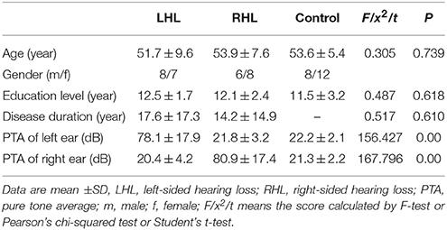
Table 1. Demographic data of all subjects.

FIGURE 1

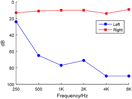
Figure 1. Frequency-dependent hearing level of a LHL subject.

Scanning was implemented by a Siemens Verio Tim 3.0T MR scanner (Siemens Medical Solutions, Erlangen, Germany). All subjects lie as still as possible with eyes closed and not to fall asleep. In total 176 sagittal slices covering the whole brain were acquired, using an MP-RAGE sequence. The imaging parameters were: TE = 2.48 ms, TR = 1900 ms, TI = 900 ms, FA = 9°, FOV = 256 × 256 mm, matrix = 256 × 256, slice thickness = 1 mm.

Preprocessing was performed using FMRIB Software Library (FSL) v5.0. The brain extraction tool (BET) was employed to extract brain and remove skulls. The results were shown in Figure 2, where the red lines outline the edges of extracted brains.

FIGURE 2

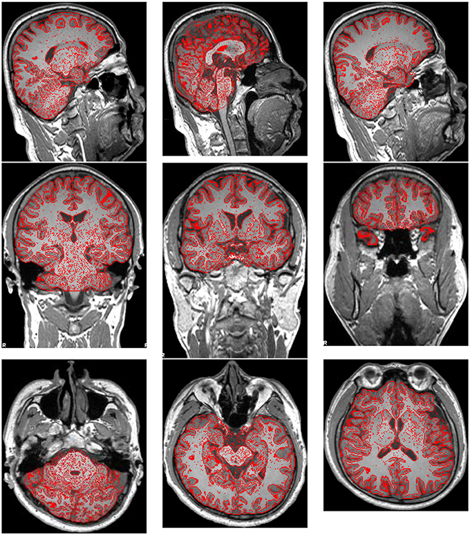
Figure 2. Brain Extraction Result.

Afterwards, all brains of 49 subjects were normalized to a standard Montreal Neurologic Institute (MNI) template and resampled to 2 mm isotropic voxels using FLIRT and FNIRT tools. Then, the normalized images were smoothed with a Gaussian kernel. Figure 3 shows the results. Three experienced otologists were instructed to select the optimal slice of each patient that covers his/her majority hearing regions, and the selected slice is around 40-th, which contains the significant discrepancy information between SNHLs and HCs. The selected slice of each patient is different.

FIGURE 3

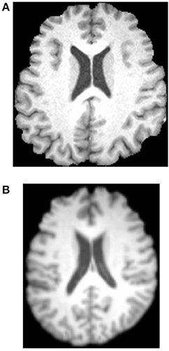
Figure 3. Normalization and Gaussian kernel results. (A) Before. (B) After.

Methodology

Computer vision (CV) technique (Wu, 2012a; Ji, 2014; Meireles et al., 2016) is used to help develop the CAD system that can distinguish LHLs and RHLs from HCs. The feature is defined as a piece of information for solving the computational task (here is to detect HL). Traditional CV methods used local features, like edges, corners, blobs, and interesting points & regions (Lee D. H. et al., 2016). Nevertheless, recently researches showed global features may also give the equivalent performances (Li B. et al., 2015). Wavelet entropy (WE) as a novel global feature has attracted attentions from various disciplines.

Wavelet Entropy

WE is a new method developed to analyze transient features of complicated signals (Hosseini et al., 2015; Phillips et al., 2015; Sun, 2015), such as the brain image in this study. The value of WE has a physical meaning of the order/disorder degree of the signal with multiscale time-frequency resolution.

WE consists of two steps: discrete wavelet decomposition and entropy calculation (See Figure 4). In the first step, the discrete wavelet decomposition was performed to the given MR brain image, and four subbands (LL1, LH1, HL1, and HH1) were yielded. Here L and H represents the low- and high-frequency coefficients. The LL1 was further decomposed into four smaller subbands as LL2, HL2, LH2, and HH2. Thus, we obtain 3*n + 1 subbands for a n-level decomposition. In the second step, entropy was calculated over each subband. In total, the WE can reduce a 256 × 256 brain image to a (3*n + 1)-element vector. The pseudocode of WE is listed below in Table 2.

FIGURE 4

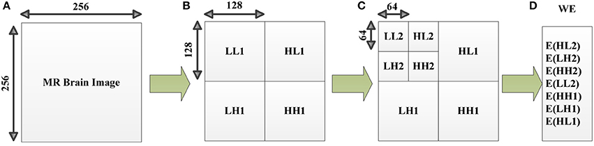
Figure 4. Diagram of a 2-level decomposition: (A) original MR brain image; (B) one-level decomposition subband; (C) two-level decomposition subband; (D) Wavelet entropy (WE) vector. (B,C) are in wavelet coefficient domain. L, low-frequency subband; H, high-frequency subband; digits after L/H represents the decomposition level, E, entropy; WE, wavelet entropy.

TABLE 2

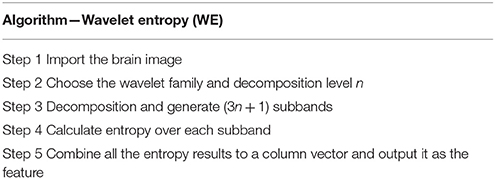
Table 2. Pseudocode of wavelet entropy.

From Table 2, we know that two factors (wavelet family and decomposition level) are needed to perform a WE. We will discuss the wavelet family in following section and the decomposition level in Section Optimal Decomposition Level.

Wavelet Family

There are many wavelet families: crude wavelets, infinite regular wavelets, orthogonal wavelets, biorthogonal wavelet pairs, and complex wavelets. In this study, we choose a particular case of biorthogonal wavelet pairs (Gawande et al., 2015), viz., B-splines biorthogonal compactly supported wavelet pairs (bior, in short). Compared to other wavelets, bior have excellent advantages of symmetry with FIR filters (Uzinski et al., 2015), vanishing moments for decomposition, and regularity for reconstruction.

There are many different combinations of parameters for bior wavelets. Usually a “bior r.d” means a B-spline biorthogonal compactly supported wavelet with reconstruction order of r and decomposition order of d. In this study, we choose the bior5.5 wavelet. Figures 5, 6 shows all relevant functions of decomposition and reconstruction processes for bior5.5.

FIGURE 5

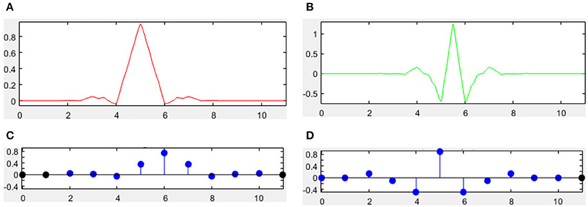
Figure 5. Decomposition for bior5.5. (A) Scaling Function. (B) Wavelet Function. (C) Low-pass filter. (D) High-pass filter.

FIGURE 6

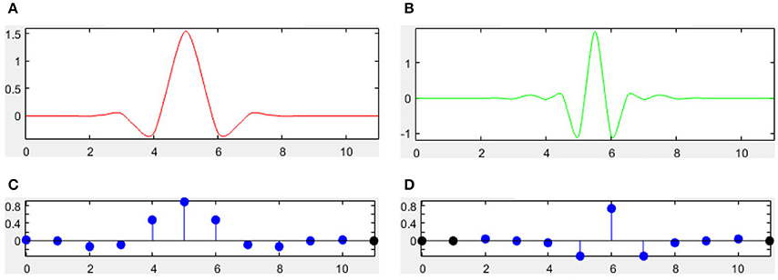
Figure 6. Reconstruction for bior5.5. (A) Scaling Function. (B) Wavelet Function. (C) Low-pass filter. (D) High-pass filter.

Support Vector Machine

One-level, two-level, three-level, and four-level decompositions of WE were submitted to support vector machine (SVM), to find which level performs the best. SVM is a non-probabilistic binary linear classifier (Yang, 2015b; Berikol et al., 2016; Pal et al., 2016), which belongs to supervised learning model used for regression or classification. Suppose we have an A-dimensional S-sized dataset as

$\begin{array}{cc}\left\{(x_n,y_n)|x_n\in {ℝ}^A,y_n\in \{-1,+1\}\right\},n=1,\mathrm{...},S& (1)\end{array}$

where n is the index of data. Each x_n is a A-dimensional vector and y_n represents its corresponding class label. SVM will build a model by following equation:

$\begin{array}{cc}\underset{w,b}{\min }\frac{1}{2}{\Vert w\Vert }^2& (2)\end{array}$

$\begin{array}{cc}\text{s}.\text{t}.y_n\left(w{x}_n-b\right)\ge 1& (3)\end{array}$

where w = [w] denotes the weights and b = [b] the biases. Note that the distances between two hyperplanes are 2/||w||, so formula (2) indicates we need to maximize the distance between two hyperplanes. In the meantime, equation (3) prevents the data falling to the margin as largely as possible.

Soft margin technique (Liu A., 2015) was further introduced for the condition when hyperplane may not split the samples perfectly. The model was then transformed to

$\begin{array}{cc}\begin{array}{l}\underset{w,\xi ,b}{\min }\frac{1}{2}{\Vert w\Vert }^2+\epsilon {\displaystyle {\sum }_{n=1}^S{\xi }_n}\hfill \\ s.t.\{\begin{array}{c}{y}_n\left(w{x}_n-b\right)\ge 1-{\xi }_n\\ {\xi }_n\ge 0\end{array},n=1,\mathrm{...},S\hfill \end{array}& (4)\end{array}$

where ξ_n denotes positive slack variables and ε denotes the error penalty. In the future, some advanced classifiers will be tested, such as nonparallel SVM, fuzzy SVM (Yang, 2015a), kernel SVM (Wu, 2012b), SVM decision tree (Dong, 2014), proximal SVM (Dufrenois and Noyer, 2016), twin SVM (Wang et al., 2016), etc.

Directed Acyclic Graph

Remember SVM is only for binary classification, hence, we introduce in the directed acyclic graph (DAG) method to reduce our three-class task (HC, LHL, RHL) to multiple binary classification problems. DAG technique is based on one vs. one approach (Lee J. et al., 2016). Suppose there are in total C classes, the DAG constructs individual classifier (IC) for each pair of classes, so in total (C − 1)C/2 individual classifiers (Gasemyr, 2016).

After each ij-th individual classifier is trained with the i-th and j-th class (i = 1,2, …, C − 1, j = i + 1, …, C), we submit a new data x into each trained individual classifier, obtaining the score (L_ij) of ij-th individual classifier and its output is the sign function of the score value L_ij, viz.,

$\begin{array}{cc}{o}_{ij}(x)=\text{sgn}(L_{ij}(x))& (5)\end{array}$

If the score L_ij(x) is larger than zero, then the output o_ij(x) is +1, denoting that x does not belong to j-th class; otherwise output is −1, denoting x does not belong to i-th class (Joutsijoki et al., 2015).

Figure 7 shows an example of using DAG technique to classify from C = 4 classes. The “1v4” individual classifier notifies that x does not belong to 1-st class, then the “2v4” individual classifier indicates that x does not belong to 2-nd class, finally the “3v4” individual classifier tells that x does not belong to 4-th class. Obviously, x belongs to 3-rd class. Our method is different from Dietl and Weiss (2004). They employed wavelet packets and SVMs to detect cochlear hearing loss. They classified pantonal and high-frequency hearing loss from normal controls. However, they did not use the imaging data.

FIGURE 7

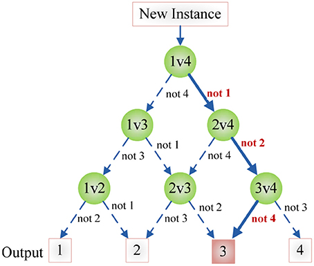
Figure 7. An example of DAG Technique with C = 4. Root node and intermediate nodes represent individual classifiers, and the leaf nodes represented the output label.

Experiments

The CAD system was in-house developed using Matlab 2015a, and run on IBM laptop with 3 GHz Intel i3 dual-processor and 8 GB RAM. With the help of DAG, the classifier is decomposed as three binary classification problems as shown in Figure 8. Here we establish three classifiers, LHL-v-RHL, LHL-v-HC, and HC-v-RHL. The three classifiers are then connected in the style of DAG.

FIGURE 8

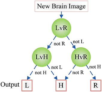
Figure 8. Diagram of the DAG-SVM for the hearing loss classification. L, LHL; R, RHL; H, HC.

A 10 × 10-fold cross validation were implemented for statistical analysis. First, we divide the dataset into 10-folds, 9-folds for training 1-fold for validation. DAG-SVM was trained each time and the confusion matrixes over the validation fold were combined to form a full confusion matrix. Then, the above procedure repeats 10 times.

The parameters of SVM are set as follows: ε equals to 0.05 by experience, C equals to 2 since each individual SVM handles a two-class classification problem. S varies in each run since the sum of the sizes of nine training folds are different, but we list the detailed statistical result in Table 4.

Results and Discussions

Wavelet Decomposition

One, two, and three levels decomposition was implemented over all brain images. Figure 9A shows the original brain image. Figure 9B shows the 1-level decomposition with four subbands. Figure 9C shows the 2-level decomposition with seven subbands. Figures 9D,E show the 3-level with 10 subbands, and 4-level with 13 subbands, respectively.

FIGURE 9

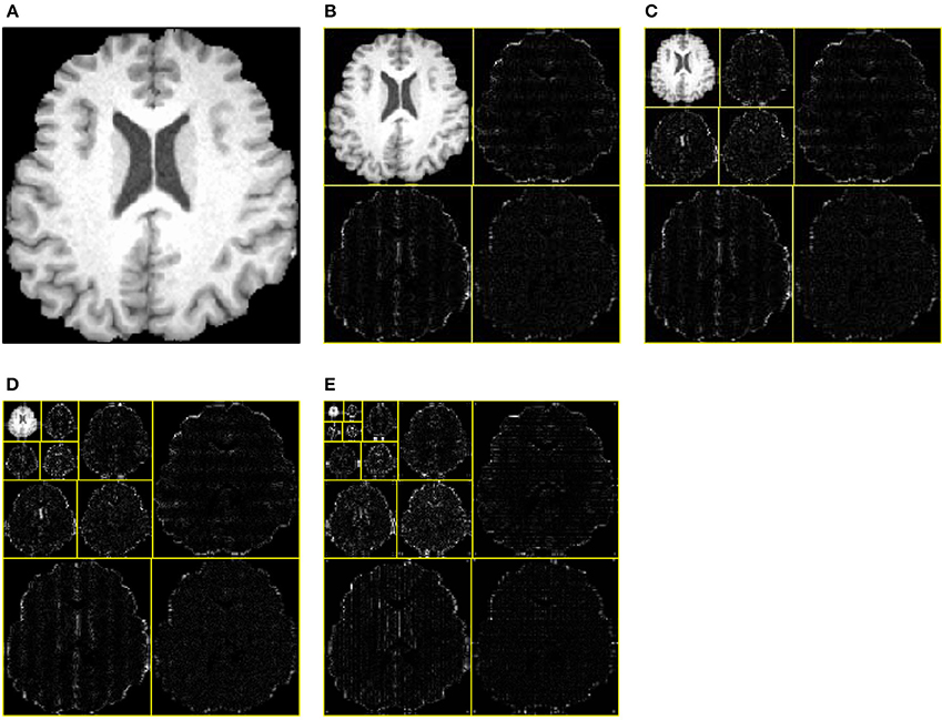
Figure 9. Decomposition results. (A) Original Image. (B) 1-level decomposition. (C) 2-level decomposition. (D) 3-level decomposition. (E) 4-level decomposition.

Optimal Decomposition Level

To decide which decomposition level performs the best for our task, we submit the generated 4, 7, 10, and 13 WEs in the last step to the DAG-SVM classifier. The overall accuracy was listed in Table 3 and it was defined as the ratio between the number of correctly classified brains and total brains. Four WEs obtains an accuracy of 92.24%, 7 WEs obtains an accuracy of 94.08%, 10 WEs obtains the highest accuracy of 95.10%, and 13 WEs obtains an accuracy of 94.29%.

TABLE 3

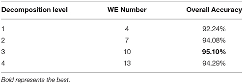
Table 3. Classification Accuracy vs. decomposition level.

Statistical Analysis

Table 4 illustrates how we obtain the result of 95.10% for a three-level WE. Each row shows the results of different runs, and each column shows the result of different folds. In the last column, we calculated the accuracy of each run. In the last row, we averaged the results of each run.

TABLE 4

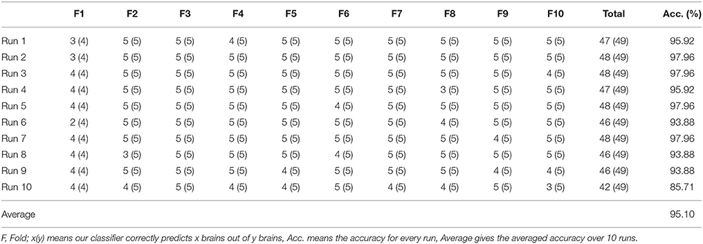
Table 4. The experiment results of 3-level decomposition.

Confusion Matrix

The confusion matrix over 10 runs is drawn in Table 5. We read the table in a row-wise way. The second row indicates that 194 HCs are recognized correctly, 4 HCs are recognized as LHLs, and 2 HCs are recognized as RHLs. The third row indicates that 141 LHLs are recognized correctly, 6 LHLs are recognized as HCs, 3 LHLs are recognized as RHLs. The final row indicates that 131 RHLs are recognized correctly, 4 RHLs are recognized as HCs, and 5 RHLs are recognized as LHLs. Table 6 lists the performances over each single class (i.e., a single class versus the combination of other two classes), which can be directly calculated from Table 5.

TABLE 5

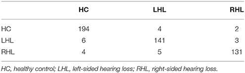
Table 5. Confusion Matrix.

TABLE 6

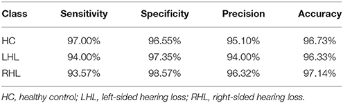
Table 6. Performance over each class.

Comparison with Manual Method

We compared our method with manual method. Three experienced observers (O1, O2, O3) with clinical experiences longer than 10 years in neuroradiology are invited to give decisions over those 49 subjects, and their reports are listed in Table 7. The accuracies of three observers are of 36.73, 32.65, and 38.78%, respectively.

TABLE 7

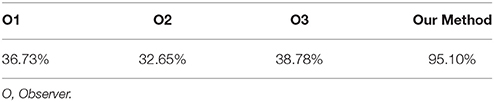
Table 7. Comparison of accuracy with manual interpretation.

Comparison with State-of-the-Art Method

There are many other popular classifiers used for classifying MR images. Kale et al. (2013) employed feedforward neural network (FNN). Scherfler et al. (2016) used decision tree (DT) as the classifier. Vasta et al. (2016) utilized naive Bayesian classifier (NBC). In this study, we compared the proposed DAG-SVM with FNN (Kale et al., 2013), DT (Scherfler et al., 2016), and NBC (Vasta et al., 2016). The features were the same as three-level WEs, the statistical analysis is all set to 10 × 10-fold cross validation, and the optimal parameters of classifiers were obtained by grid searching. The results are listed in Table 8.

TABLE 8

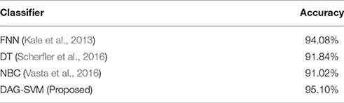
Table 8. Classifier comparison.

Discussions

The WEs in Figure 9 were obtained after performing entropy calculation over each subband, namely, 4 WEs for 1-level decomposition, 7 WEs for 2-level decomposition, 10 WEs for 3-level decomposition, and 13 WEs for 4-level decomposition. As it expects, more WEs will provide more information. Nevertheless, too many WEs will deteriorate the performance of the classifier. In this paper, we tested 4, 7, 10, and 13 WEs.

The support vectors are difficult to display due to four reasons: (i) They are in high-dimensional feature space; (ii) The classifier is regarded as a “black box” from the view of computer scientists; (iii) We have three individual classifiers, and their support vectors are different; (iv) The 10 × 10-fold statistical analysis make us to run the classifier training 100 times, and the support vectors at each time are different. Further, several other research teams also used SVMs without displaying the support vectors (Chen et al., 2015; Liu G., 2015; Tan et al., 2015; Chen M. Y. et al., 2016). This is like a face recognition system that recognizes faces quite well with a too complicated inner structure to display.

A limitation is that the wavelet subbands are mathematically generated, thus the results only have mathematical meaning but they cannot implicate which brain area drives the difference between the classes. Traditionally, scholars like to measure the cortical thickness (Marie et al., 2016), generate gray or white matter maps (Bonnier et al., 2016), since it carries more information and links better between classification performance and brain regions. But nowadays, the growth of artificial intelligence has a trend of creating “black box” model that let the machine extract a set of task-oriented image features automatically (Premaladha and Ravichandran, 2016), with better classification performance than traditional methods. Therefore, our method follows the new idea of classification.

Table 3 shows the overall accuracy results for each decomposition level. The results indicate 3-level decomposition with 10 WEs performed the best with the highest accuracy of 95.10%. Again, this falls in line with our expectation. First, adding WEs will provide more information, which do good to the classifier. However, too many features may confuse the classifier. From Figure 9E, we can see that the smallest subbands of 4-level decomposition generates is unclear and may be blurred by neighboring subbands.

Table 6 shows that HC has a sensitivity of 97.00%, a specificity of 96.55, a precision of 95.10%, and an accuracy of 96.73%. LHL has a sensitivity of 94.00%, a specificity of 97.35%, a precision of 94.00%, and an accuracy of 96.33%. RHL has a sensitivity of 93.57%, a specificity of 98.57%, a precision of 96.32%, and an accuracy of 97.14%. We found that computer can detect all three classes with an accuracy higher than 96%. This indicates our method achieved excellent result. The high accuracy stems from two facts: (i) LHL patients are different from RHL patients (Fan et al., 2015); and (ii) SNHLs have difference with healthy subjects in brain structures (Yang et al., 2014). The situation was similar to the finger tipping task in fMRI, which the activation of left hand and that of right hand is distinctive for computers (Kuehn et al., 2015; Sun et al., 2015).

Table 7 shows that computer programs may replace human interpretation in terms of brain MR images. The reason why those three experienced observers fail lies in the difference between SNHL and HC are difficult to be perceived by human eye, through which the brain MR images of HL patients appear normal. The accuracies obtained by human observers are close to baseline demonstrated this point. This also validated the success of our CAD system, which is due to the high-sensitivity of computers for slight pixel gray-level difference and region atrophy.

Table 8 shows FNN (Kale et al., 2013) achieves an accuracy of 94.08%, DT (Scherfler et al., 2016) achieves an accuracy of 91.84%, and NBC (Vasta et al., 2016) achieves an accuracy of 91.02%. We can see our method “DAG-SVM” obtains the highest accuracy of 95.10%. The result shows the superiority of SVM to other popular classifiers.

Conclusions

In this paper, we developed a novel CAD for detecting unilateral hearing loss. To the best known of the authors, we are the first to apply SVM in UHL detection. The overall accuracy of the three-class problem is 95.10%, which offers a promising result.

In the future, we will consider other classification tasks, such as including the classes of pan-tonal and high-frequency hearing loss. Another research direction is to use advanced optimization techniques to train SVM, such as hybrid genetic algorithm (Lu, 2016), biogeography-based optimization (Wei, 2015), particle swarm optimization (PSO, Ji, 2015), chaotic adaptive PSO (Wu J., 2016), etc.

More feature selection methods will be tested such as displacement field (Wang et al., 2015), eigenbrain (Phillips, 2016), and fractional Fourier entropy (Sun, 2016). More classifiers will be tested, for example, the k-nearest neighbors (Zhou, 2016), artificial neural network (Wu X., 2016), decision tree (Zhang, 2014), etc.

Author Contributions

SW, MY, and YZ conceived the study. SD, JY, and YZ designed model. MY and BL acquired the data. SW, JG, and YZ analyzed the data. JR and YZ processed the data. MY, SD, TY, and YZ interpreted the results. SW and YZ developed programs. SW, TY, and YZ wrote the draft. All authors gave critical revisions.

Conflict of Interest Statement

The authors declare that the research was conducted in the absence of any commercial or financial relationships that could be construed as a potential conflict of interest.

Acknowledgments

This paper was supported by NSFC (61602250, 61271231, 51407095, 61503188), Open Fund of Key laboratory of Symbolic Computation and Knowledge Engineering of Ministry of Education, Jilin University (93K172016K17), Open Fund of Key Laboratory of Statistical Information Technology and Data Mining, State Statistics Bureau, (SDL201608), Program of Natural Science Research of Jiangsu Higher Education Institutions (16KJB520025), Open Research Fund of Hunan Provincial Key Laboratory of Network Investigational Technology (2016WLZC013), Open Fund of Fujian Provincial Key Laboratory of Data Intensive Computing (BD201607), Nanjing Normal University Research Foundation for Talented Scholars (2013119XGQ0061, 2014119XGQ0080), Natural Science Foundation of Jiangsu Province (BK20150983).

Abbreviations

SNHL, Sensorineural hearing loss; UHL, Unilateral hearing loss; LHL, Left-sided hearing loss; RHL, Right-sided hearing loss; HC, Healthy control; MRI, Magnetic resonance imaging; PTA, Pure tone average; MNI, Montreal neurologic institute; DAG, Directed acyclic graph; FNN, Feedforward neural network; DT, Decision tree, NBC, Naive Bayesian classifier.

References

Amir, G. J., and Lehmann, H. P. (2016). After detection: the improved accuracy of lung cancer assessment using radiologic computer-aided diagnosis. Acad. Radiol. 23, 186–191. doi: 10.1016/j.acra.2015.10.014

PubMed Abstract | CrossRef Full Text | Google Scholar

Berikol, G. B., Yildiz, O., and Özcan, I. T. (2016). Diagnosis of acute coronary syndrome with a support vector machine. J. Med. Syst. 40:84. doi: 10.1007/s10916-016-0432-6

PubMed Abstract | CrossRef Full Text | Google Scholar

Bonnier, G., Kober, T., Schluep, M., Du Pasquier, R., Krueger, G., Meuli, R., et al. (2016). A new approach for deep gray matter analysis using partial-volume estimation. PLoS ONE 11:e0148631. doi: 10.1371/journal.pone.0148631

PubMed Abstract | CrossRef Full Text | Google Scholar

Chen, M. Y., Tan, X. M., and Zhang, L. (2016). An iterative self-training support vector machine algorithm in brain-computer interfaces. Intell. Data Anal. 20, 67–82. doi: 10.3233/IDA-150794

CrossRef Full Text | Google Scholar

Chen, S., Yang, J.-F., and Phillips, P. (2015). Magnetic resonance brain image classification based on weighted-type fractional Fourier transform and nonparallel support vector machine. Int. J. Imaging Syst. Technol. 25, 317–327. doi: 10.1002/ima.22144

CrossRef Full Text | Google Scholar

Chilosi, A. M., Comparini, A., Scusa, M. F., Berrettini, S., Forli, F., Battini, R., et al. (2010). Neurodevelopmental disorders in children with severe to profound sensorineural hearing loss: a clinical study. Dev. Med. Child Neurol. 52, 856–862. doi: 10.1111/j.1469-8749.2010.03621.x

PubMed Abstract | CrossRef Full Text | Google Scholar

Choi, J. Y., Kim, D. H., Plataniotis, K. N., and Ro, Y. M. (2016). Classifier ensemble generation and selection with multiple feature representations for classification applications in computer-aided detection and diagnosis on mammography. Expert Syst. Appl. 46, 106–121. doi: 10.1016/j.eswa.2015.10.014

CrossRef Full Text | Google Scholar

Dietl, H., and Weiss, S. (2004). “Detection of cochlear hearing loss applying wavelet packets and support vector machines,” in Thirty-Eighth Asilomar Conference on Signals, Systems and Computers, (Monterey, CA: IEEE), 1575–1579.

Dong, Z. (2014). Classification of Alzheimer disease based on structural magnetic resonance imaging by kernel support vector machine decision tree. Prog. Electromagn. Res. 144, 171–184. doi: 10.2528/PIER13121310

CrossRef Full Text | Google Scholar

Dufrenois, F., and Noyer, J. C. (2016). One class proximal support vector machines. Pattern Recognit. 52, 96–112. doi: 10.1016/j.patcog.2015.09.036

CrossRef Full Text | Google Scholar

Eftekharian, A., and Amizadeh, M. (2016). Pulse steroid therapy in idiopathic sudden sensorineural hearing loss: a randomized controlled clinical trial. Laryngoscope 126, 150–155. doi: 10.1002/lary.25244

PubMed Abstract | CrossRef Full Text | Google Scholar

Fan, W., Zhang, W., Li, J., Zhao, X., Mella, G., Lei, P., et al. (2015). Altered contralateral auditory cortical morphology in unilateral sudden sensorineural hearing loss. Otol. Neurotol. 36, 1622–1627. doi: 10.1097/MAO.0000000000000892

PubMed Abstract | CrossRef Full Text | Google Scholar

Gasemyr, J. (2016). Uniformity of node level conflict measures in bayesian hierarchical models based on directed acyclic graphs. Scand. J. Stat. 43, 20–34. doi: 10.1111/sjos.12162

CrossRef Full Text | Google Scholar

Gawande, J. P., Rahulkar, A. D., and Holambe, R. S. (2015). Design of new class of regular biorthogonal wavelet filter banks using generalized and hybrid lifting structures. Signal Image Video Process. 9, 265–273. doi: 10.1007/s11760-015-0814-0

CrossRef Full Text | Google Scholar

Hosseini, S. A., Amjady, N., and Velayati, M. H. (2015). A Fourier based wavelet approach using Heisenberg's uncertainty principle and Shannon's entropy criterion to monitor power system small signal oscillations. IEEE Trans. Power Syst. 30, 3314–3326. doi: 10.1109/TPWRS.2014.2377180

CrossRef Full Text | Google Scholar

Hribar, M., Suput, D., Carvalho, A. A., Battelino, S., and Vovk, A. (2014). Structural alterations of brain grey and white matter in early deaf adults. Hear. Res. 318, 1–10. doi: 10.1016/j.heares.2014.09.008

PubMed Abstract | CrossRef Full Text | Google Scholar

Ji, G. (2014). Fruit classification using computer vision and feedforward neural network. J. Food Eng. 143, 167–177. doi: 10.1016/j.jfoodeng.2014.07.001

CrossRef Full Text | Google Scholar

Ji, G. (2015). A comprehensive survey on particle swarm optimization algorithm and its applications. Math. Probl. Eng. 2015:931256. doi: 10.1155/2015/931256

CrossRef Full Text | Google Scholar

Joutsijoki, H., Siermala, M., and Juhola, M. (2015). Directed acyclic graph support vector machines in classification of benthic macroinvertebrate samples. Artif. Intell. Rev. 44, 215–233. doi: 10.1007/s10462-014-9425-3

CrossRef Full Text | Google Scholar

Kale, M. C., Fleig, J. D., and Imal, N. (2013). Assessment of feasibility to use computer aided texture analysis based tool for parametric images of suspicious lesions in DCE-MR mammography. Comput. Math. Methods Med. 2013:872676. doi: 10.1155/2013/872676

PubMed Abstract | CrossRef Full Text | Google Scholar

Khalid, S., Qadir, M., and Salat, M. S. (2015). Spontaneous improvement in sensorineural hearing loss developed as a complication of neonatal hyperbilirubinemia. J. Pak. Med. Assoc. 65, 1018–1021.

PubMed Abstract | Google Scholar

Koylu, M. T., Gokce, G., Sobaci, G., Oysul, F. G., and Akincioglu, D. (2016). Ophthalmic pathologies in female subjects with bilateral congenital sensorineural hearing loss. Turk. J. Med. Sci. 46, 139–144. doi: 10.3906/sag-1411-82

PubMed Abstract | CrossRef Full Text | Google Scholar

Kuehn, E., De Havas, J., Silkoset, E., Gomi, H., and Haggard, P. (2015). On the bimanual integration of proprioceptive information. Exp. Brain Res. 233, 1273–1288. doi: 10.1007/s00221-015-4205-0

PubMed Abstract | CrossRef Full Text | Google Scholar

Lee, D. H., Lee, D. W., and Han, B. S. (2016). Brodmann's area template based region of interest setting and probabilistic pathway map generation in diffusion tensor tractography: application to the arcuate fasciculus fiber tract in the human brain. Front. Neuroanat. 10:4. doi: 10.3389/fnana.2016.00004

PubMed Abstract | CrossRef Full Text | Google Scholar

Lee, J., Kim, H., Kim, N. R., and Lee, J. H. (2016). An approach for multi-label classification by directed acyclic graph with label correlation maximization. Inf. Sci. 351, 101–114. doi: 10.1016/j.ins.2016.02.037

CrossRef Full Text | Google Scholar

Li, B., Li, W., and Zhao, D. Z. (2015). Global and local features based medical image classification. J. Med. Imaging Health Inform. 5, 748–754. doi: 10.1166/jmihi.2015.1445

CrossRef Full Text | Google Scholar

Lin, C. F., Lee, K. J., Yu, S. S., and Lin, Y. S. (2016). Effect of comorbid diabetes and hypercholesterolemia on the prognosis of idiopathic sudden sensorineural hearing loss. Laryngoscope 126, 142–149. doi: 10.1002/lary.25333

PubMed Abstract | CrossRef Full Text | Google Scholar

Liu, A. (2015). Magnetic resonance brain image classification via stationary wavelet transform and generalized eigenvalue proximal support vector machine. J. Med. Imaging Health Inform. 5, 1395–1403. doi: 10.1166/jmihi.2015.1542

CrossRef Full Text | Google Scholar

Liu, G. (2015). Pathological brain detection in MRI scanning by wavelet packet Tsallis entropy and fuzzy support vector machine. SpringerPlus 4:716. doi: 10.1186/s40064-015-1523-4

PubMed Abstract | CrossRef Full Text | Google Scholar

Li, Z., Zhu, Q., Geng, Z., Song, Z., Wang, L., and Wang, Y. (2015). Study of functional connectivity in patients with sensorineural hearing loss by using resting-state fMRI. Int. J. Clin. Exp. Med. 8, 569–578.

PubMed Abstract | Google Scholar

Lu, S. (2016). A note on the weight of inverse complexity in improved hybrid genetic algorithm. J. Med. Syst. 40:150. doi: 10.1007/s10916-016-0512-7

PubMed Abstract | CrossRef Full Text | Google Scholar

Marie, D., Maingault, S., Crivello, F., Mazoyer, B., and Tzourio-Mazoyer, N. (2016). Surface-based morphometry of cortical thickness and surface area associated with Heschl's gyri duplications in 430 healthy volunteers. Front. Hum. Neurosci. 10:69. doi: 10.3389/fnhum.2016.00069

PubMed Abstract | CrossRef Full Text | Google Scholar

Martin, W., Jelsma, J., and Rogers, C. (2012). Motor proficiency and dynamic visual acuity in children with bilateral sensorineural hearing loss. Int. J. Pediatr. Otorhinolaryngol. 76, 1520–1525. doi: 10.1016/j.ijporl.2012.07.007

PubMed Abstract | CrossRef Full Text | Google Scholar

Martínez-Cruz, C. F., Poblano, A., and Conde-Reyes, M. P. (2009). Cognitive performance of school children with unilateral sensorineural hearing loss. Arch. Med. Res. 40, 374–379. doi: 10.1016/j.arcmed.2009.05.008

PubMed Abstract | CrossRef Full Text | Google Scholar

Meireles, A. B., Vieira, A. W., Corpas, L., Vandenberghe, B., Bastos, F. S., Lambrechts, P., et al. (2016). Dental wear estimation using a digital intra-oral optical scanner and an automated 3D computer vision method. Comput. Methods Biomech. Biomed. Engin. 19, 507–514. doi: 10.1080/10255842.2015.1043627

PubMed Abstract | CrossRef Full Text | Google Scholar

Pal, R., Kupka, K., Aneja, A. P., and Militky, J. (2016). Business health characterization: a hybrid regression and support vector machine analysis. Expert Syst. Appl. 49, 48–59. doi: 10.1016/j.eswa.2015.11.027

CrossRef Full Text | Google Scholar

Phillips, P. (2016). Three-dimensional eigenbrain for the detection of subjects and brain regions related with Alzheimer's disease. J. Alzheimers Dis. 50, 1163–1179. doi: 10.3233/JAD-150988

PubMed Abstract | CrossRef Full Text | Google Scholar

Phillips, P., Dong, Z., and Yang, J. (2015). Pathological brain detection in magnetic resonance imaging scanning by wavelet entropy and hybridization of biogeography-based optimization and particle swarm optimization. Prog. Electromagn. Res. 152, 41–58. doi: 10.2528/PIER15040602

CrossRef Full Text | Google Scholar

Premaladha, J., and Ravichandran, K. S. (2016). Novel approaches for diagnosing melanoma skin lesions through supervised and deep learning algorithms. J. Med. Syst. 40:96. doi: 10.1007/s10916-016-0460-2

PubMed Abstract | CrossRef Full Text | Google Scholar

Profant, O., Škoch, A., Balogová, Z., Tintera, J., Hlinka, J., and Syka, J. (2014). Diffusion tensor imaging and MR morphometry of the central auditory pathway and auditory cortex in aging. Neuroscience 260, 87–97. doi: 10.1016/j.neuroscience.2013.12.010

PubMed Abstract | CrossRef Full Text | Google Scholar

Prosser, J. D., Cohen, A. P., and Greinwald, J. H. (2015). Diagnostic evaluation of children with sensorineural hearing loss. Otolaryngol. Clin. North Am. 48:975. doi: 10.1016/j.otc.2015.07.004

PubMed Abstract | CrossRef Full Text | Google Scholar

Scherfler, C., Göbel, G., Muller, C., Nocker, M., Wenning, G. K., Schocke, W., et al. (2016). Diagnostic potential of automated subcortical volume segmentation in atypical parkinsonism. Neurology 86, 1242–1249. doi: 10.1212/WNL.0000000000002518

PubMed Abstract | CrossRef Full Text | Google Scholar

Shiell, M. M., Champoux, F., and Zatorre, R. J. (2016). The right hemisphere planum temporale supports enhanced visual motion detection ability in deaf people: evidence from cortical thickness. Neural Plast. 2016:7217630. doi: 10.1155/2016/7217630

PubMed Abstract | CrossRef Full Text | Google Scholar

Sun, H., Fessler, J. A., Noll, D. C., and Nielsen, J. F. (2015). Steady-state functional MRI using spoiled small-tip fast recovery imaging. Magn. Reson. Med. 73, 536–543. doi: 10.1002/mrm.25146

PubMed Abstract | CrossRef Full Text | Google Scholar

Sun, P. (2015). Pathological brain detection based on wavelet entropy and Hu moment invariants. Biomed. Mater. Eng. 26, 1283–1290. doi: 10.3233/BME-151426

PubMed Abstract | CrossRef Full Text | Google Scholar

Sun, Y. (2016). A multilayer perceptron based smart pathological brain detection system by fractional fourier entropy. J. Med. Syst. 40:173. doi: 10.1007/s10916-016-0525-2

PubMed Abstract | CrossRef Full Text | Google Scholar

Tan, L., Holland, S. K., Deshpande, A. K., Chen, Y., Choo, D. I., and Lu, L. J. (2015). A semi-supervised support vector machine model for predicting the language outcomes following cochlear implantation based on pre-implant brain fMRI imaging. Brain Behav. 5:e00391. doi: 10.1002/brb3.391

PubMed Abstract | CrossRef Full Text | Google Scholar

Teranishi, M., Uchida, Y., Nishio, N., Kato, K., Otake, H., Yoshida, T., et al. (2012). Polymorphisms in genes involved in oxidative stress response in patients with sudden sensorineural hearing loss and Meniere's disease in a Japanese population. DNA Cell Biol. 31, 1555–1562. doi: 10.1089/dna.2012.1631

PubMed Abstract | CrossRef Full Text | Google Scholar

Uzinski, J. C., Paiva, H. M., Duarte, M. A. Q., Galvao, R. K. H., and Villarreal, F. (2015). A state-space description for perfect-reconstruction wavelet FIR filter banks with special orthonormal basis functions. J. Comput. Appl. Math. 290, 290–297. doi: 10.1016/j.cam.2015.04.046

CrossRef Full Text | Google Scholar

Vaden, K. I. Jr., Kuchinsky, S. E., Ahlstrom, J. B., Teubner-Rhodes, S. E., Dubno, J. R., and Eckert, M. A. (2016). Cingulo-opercular function during word recognition in noise for older adults with hearing loss. Exp. Aging Res. 42, 86–106. doi: 10.1080/0361073X.2016.1108784

PubMed Abstract | CrossRef Full Text | Google Scholar

Vasta, R., Augimeri, A., Cerasa, A., Nigro, S., Gramigna, V., Nonnis, M., et al. (2016). Hippocampal subfield atrophies in converted and not-converted mild cognitive impairments patients by a markov random fields algorithm. Curr. Alzheimer Res. 13, 566–574. doi: 10.2174/1567205013666160120151457

PubMed Abstract | CrossRef Full Text | Google Scholar

Wang, S., Chen, M., Li, Y., Shao, Y., Zhang, Y., Du, S., et al. (2016). Morphological analysis of dendrites and spines by hybridization of ridge detection with twin support vector machine. PeerJ 4:e2207. doi: 10.7717/peerj.2207

PubMed Abstract | CrossRef Full Text | Google Scholar

Wang, S., Zhang, Y., Liu, G., Phillips, P., and Yuan, T.-F. (2015). Detection of Alzheimer's disease by three-dimensional displacement field estimation in structural magnetic resonance imaging. J. Alzheimer's Dis. 50, 233–248. doi: 10.3233/JAD-150848

PubMed Abstract | CrossRef Full Text | Google Scholar

Wei, L. (2015). Fruit classification by wavelet-entropy and feedforward neural network trained by fitness-scaled chaotic ABC and biogeography-based optimization. Entropy 17, 5711–5728. doi: 10.3390/e17085711

CrossRef Full Text | Google Scholar

Wu, J. (2016). Fruit classification by biogeography-based optimization and feedforward neural network. Expert Syst. 33, 239–253. doi: 10.1111/exsy.12146

CrossRef Full Text | Google Scholar

Wu, L. (2012a). Classification of fruits using computer vision and a multiclass support vector machine. Sensors 12, 12489–12505. doi: 10.3390/s120912489

PubMed Abstract | CrossRef Full Text | Google Scholar

Wu, L. (2012b). An MR brain images classifier via principal component analysis and kernel support vector machine. Prog. Electromagn. Res. 130, 369–388. doi: 10.2528/PIER12061410

CrossRef Full Text | Google Scholar

Wu, X. (2016). Smart detection on abnormal breasts in digital mammography based on contrast-limited adaptive histogram equalization and chaotic adaptive real-coded biogeography-based optimization. Simulation 92, 873–885. doi: 10.1177/0037549716667834

CrossRef Full Text | Google Scholar

Yang, J. (2015a). Identification of green, Oolong and black teas in China via wavelet packet entropy and fuzzy support vector machine. Entropy 17, 6663–6682. doi: 10.3390/e17106663

CrossRef Full Text | Google Scholar

Yang, J. (2015b). Preclinical diagnosis of magnetic resonance (MR) brain images via discrete wavelet packet transform with Tsallis entropy and generalized eigenvalue proximal support vector machine (GEPSVM). Entropy 17, 1795–1813. doi: 10.3390/e17041795

CrossRef Full Text | Google Scholar

Yang, M. (2016). Dual-tree complex wavelet transform and twin support vector machine for pathological brain detection. Appl. Sci. 6:169. doi: 10.3390/app6060169

CrossRef Full Text | Google Scholar

Yang, M., Chen, H. J., Liu, B., Huang, Z. C., Feng, Y., Li, J., et al. (2014). Brain structural and functional alterations in patients with unilateral hearing loss. Hear. Res. 316, 37–43. doi: 10.1016/j.heares.2014.07.006

PubMed Abstract | CrossRef Full Text | Google Scholar

Yang, M., Zhang, Y., Li, J., Zou, L., Lu, S., Liu, B., et al. (2016). Detection of left-sided and right-sided hearing loss via fractional fourier transform. Entropy 18:194. doi: 10.3390/e18050194

CrossRef Full Text | Google Scholar

Yuan, T. F. (2015). Detection of subjects and brain regions related to Alzheimer's disease using 3D MRI scans based on eigenbrain and machine learning. Front. Comput. Neurosci. 9:66. doi: 10.3389/fncom.2015.00066

PubMed Abstract | CrossRef Full Text | Google Scholar

Zhang, Y. (2014). Binary PSO with mutation operator for feature selection using decision tree applied to spam detection. Knowledge-Based Syst. 64, 22–31. doi: 10.1016/j.knosys.2014.03.015

CrossRef Full Text | Google Scholar

Zhang, Y., Peng, B., Wang, S., Liang, Y.-X., Yang, J., So, K.-F., et al. (2016). Image processing methods to elucidate spatial characteristics of retinal microglia after optic nerve transection. Sci. Rep. 6:21816. doi: 10.1038/srep21816

PubMed Abstract | CrossRef Full Text | Google Scholar

Zhou, X.-X. (2016). Comparison of machine learning methods for stationary wavelet entropy-based multiple sclerosis detection: decision tree, k-nearest neighbors, and support vector machine. Simulation 92, 861–871. doi: 10.1177/0037549716666962

CrossRef Full Text | Google Scholar