Time scales of representation in the human brain: weighing past information to predict future events

Introduction

Causal structure within the physical world induces regularities in the order and timing of events. Whether there is uncertainty in the underlying physical process or not, an observer of these events will always be uncertain, to a degree, about these underlying generative processes as they have to be inferred from a finite (often small) number of observations. Importantly, such regularities may be generated by a combination of processes at different temporal scales. For example, while a visual stimulus may only occur for a brief moment, it can also be embedded in a sequence of events and thereby convey information that will update one’s expectations. At the same time, slowly changing contextual causes shape the rapid fluctuation of a visual scene with time. Encoding this uncertainty is important to an observer because it provides a basis to efficiently allocate resources to make predictions that protect against overconfidence.

Previous accounts have suggested that the brain is organized hierarchically, according to the temporal structure and regularities in which events occur. Accordingly, prefrontal cortex is hierarchically organized along a rostro-caudal gradient, in which temporally more complex and extended representations are progressively presented more rostrally (Koechlin et al., 2003; Badre, 2008). These more rostral regions thus encode information over longer time intervals (Fuster, 2001, 2004) and more complex temporal relationships (Koechlin and Hyafil, 2007). Temporal scale is therefore thought to be the critical parameter that distinguishes the hierarchical organization of the prefrontal lobe (Botvinick, 2008).

Recent extensions to these ideas propose that the specific time scale which engages a cortical area can be inferred by its location from primary sensory (short time scale, STS) to high level areas (long time scale, LTS; Kiebel et al., 2008). This extends previous accounts by regarding cortex as a single hierarchy (which includes early sensory responses), rather than partitioning this hierarchy into motor and perceptual subdivisions, or indeed focusing on prefrontal regions alone. This view makes the prediction that the brain’s estimation of uncertainty depends on how information is used about past events, and that progressively more extended time scales will map onto progressively higher regions of the cortical hierarchy.

The aim of the current paper is to directly address this hypothesis, and test whether neuronal responses are characterized by specific time scales, with progressively longer time scales being represented in more anterior parts of cortex. In particular, this hypothesis predicts that responses in regions involved in executive control, i.e., frontal cortex, will be engaged at behavioral time scales that integrate past information. In addition, it is predicted that regions lower down the hierarchy, e.g., primary visual cortex, will respond at the time scale corresponding to individual events.

The first steps toward formulating a quantitative map from uncertainty onto behavioral responses were taken by Hick (1952) and Hyman (1953), who demonstrated a linear dependence of reaction time (RT) on the number of options in a forced-choice task. Because options appeared randomly and event probability decreases with the number of options this suggests that a statistical model could be used to form hypotheses as to how humans encode uncertainty to make informed decisions. One way to achieve this is to use information theoretic (IT) indices (such as the average uncertainty or entropy), which are a function of the observers estimate of the probability distribution responsible for generating samples (Strange et al., 2005; Harrison et al., 2006; Bestmann et al., 2008; Mars et al., 2008; see Materials and Methods for detail).

Previously we have shown with this approach that an ideal observer using all past events can be used to explain the role of the hippocampus in encoding uncertainty (Strange et al., 2005; Harrison et al., 2006), changes in cortical excitability during action preparation under varying conditions of uncertainty (Bestmann et al., 2008), cortical potentials (P300) linked to contextual updating (Mars et al., 2008), and saccadic eye movements (Brodersen et al., 2008). An important feature of the computational model used in our previous studies, however, is its inability to forget. Estimation of uncertainties was based on all previous events. Here, we relax this assumption, and generalize this to a time-dependent model, where distant events are weighted less than recent ones. We first illustrate how such models can be used to explain human responses using simulated RT and functional magnetic resonance imaging (fMRI) data, which in turn provide face validity for the Bayesian framework used here to evaluate the relative evidence for competing models. We used computational fMRI¹ (Friston and Dolan, 2010) in combination with Bayesian model selection (BMS; Rosa et al., 2010) to investigate the functional organization of time scales that support the encoding and response in humans to uncertainty among visual events guiding action. To test our hypothesis, we used RT and fMRI data previously reported in Harrison et al. (2006).

Materials and Methods

Probability Model and Transition Probabilities

We here considered k = 1 … K visual colored shapes, where K equals 2 and 4 in our simulations and experiment (see later for further details on the specific task) respectively that an observer has to respond to as fast as possible, but always has some degree of uncertainty about which shape will occur. At time point t_i we observe the symbol x_i. For example, x_i = 2 corresponds to the second colored shape. The number of “counts” of the k-th event type, α_k, is updated according to the following formula

where t_i is the time of the i-th observation and δ(x_i = k) equals 1 if the i-th observation was of the k-th symbol. The count variables for time point t_N are therefore based on all previous observations, but they are exponentially weighted depending on recency. The infinite time scale (ITS) model used in previous work (Harrison et al., 2006) corresponds to the assumption that τ = ∞ (in this case the exponential terms reduce to unity). In other words, the model never forgets. The counts are all initialized to 1 at the first time point.

The posterior probability of the k-th event occurring is given by the k-th parameter of a Multinomial distribution (Bishop, 2006)

The information content or “surprise” of the N-th trial is given by

Thus the occurrence of a low probability event is more surprising. The entropy (average information content) is given by

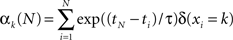
In the simple approach described above, with τ = ∞, the total number of effective counts increases by one with each sample. The consequence of this is that, in effect, the model never forgets. This is an important observation because it means that it cannot be used to investigate the effect of time or forgetting on response. Given this, the next natural step is to finesse the model to explore differences due to the number and weight given to past samples. The introduction of a decay function is the way to do this, which adds a further dimension to the model and enables one to test the number of samples a subject uses when responding to uncertainty. We achieve this by damping the effective counts as illustrated in Figure 1. This shows a schematic based on a sequence of events sampled from a Bernoulli process, e.g., a series of coin tosses, where the probability of “Heads” is fixed throughout the sample. Note there are only two outcomes in this simple example, i.e., K = 2, however, four are used in the experimental task (see “Acquisition, Preprocessing, and Analysis of fMRI Data”). The main point here is that the extent of integration has an impact on features of explanatory variables that are used to explain RT and fMRI data. As such we can use this model to measure the effects of integration over past events on behavioral and neuronal responses.

FIGURE 1

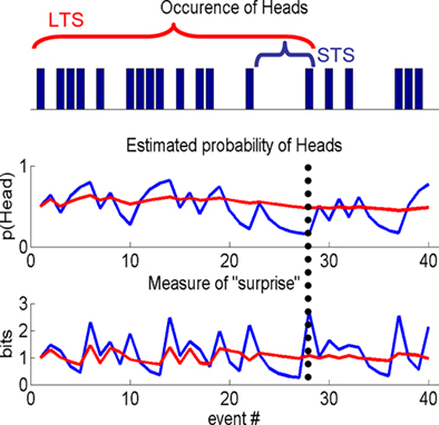
Figure 1. Information theoretic indices. A sample from a Bernoulli process, e.g., a sequence of coin tosses, over 40 events (top panel), schematic showing differences in the estimated probability of Heads, given past samples (middle panel) and a typical IT measure, i.e., “surprise,” used in a computational model to quantify subject responses (lower panel). Short (STS) or long time scale (LTS), i.e., integration over few or many past events, are shown by the blue and red traces, respectively. The differences between the two processes are best appreciated by considering the 28th event (indicated by the vertical dotted line). The estimated probability of Heads is low for the STS as it is the first Head in five events. By contrast, many samples have occurred over a longer period, which is reflected in the estimate using the LTS. STS is therefore sensitive to local changes (over events) in the process, whereas the LTS averages these out. This is seen again when considering a function of the estimated probability of Heads, e.g., the negative log of this estimate, i.e., the surprise. For the STS the probability of Heads is low and therefore the surprise is high compared to the LTS that estimates the coin to be approximately fair.

The experiment described in Harrison et al. (2006) generated symbols which additionally had probabilistic dependencies between trials, such that the current sample depended on the previous, a so-called first-order Markov process. That is, there is further order to the random sequence beyond that in each trial. In other words, the dependence between consecutive random variables imposes additional order on the set of trials in a block. It is this structure that, if estimated, can be used to reduce uncertainty in the set of samples, which will have an impact on a subject’s response.

The first-order Markov dependencies, or transition probabilities, can be estimated in a similar way as the event probabilities above. That is, one has a K-by-K table of “transition counts” where the i,j-th entry counts the number of times symbol i was preceded by symbol j. One then also employs an exponential weighting as above. One can then compute a transition probability matrix for each time point and from this one can derive an estimate of the mutual information, as previously described (Harrison et al., 2006).

Simulated Data

Reaction times were simulated for 12 subjects, each containing 12 blocks (each comprised of 40 samples), as in the experimental paradigm, using a known half-life of four past events. The aim of this simulation was to recover the known half-life using Bayesian model comparison. This was achieved using the group analysis described in Bestmann et al. (2008) to compute the probability of the data, the so-called model evidence, for a range of half-lives (from one to eight past events in steps of a half). The input, u, was sampled from a Bernoulli process, i.e., K = 2, and used to construct a design matrix, X, used to generate a response. For simplicity, we here focused on a model that comprised three columns (entropy, surprise, and offset). We now described how data were generated for a single block. This was based on the following generative model

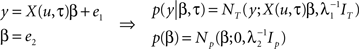
Samples from a random process are represented by u, response data is in the vector, y, of length T, the design matrix, X(u, τ), contains IT indices (e.g., entropy and surprise in response to u) along with a column of ones and I_N is the identity matrix of dimension N. General linear model (GLM) coefficient weights are β and error precisions are λ = {λ₁, λ₂}.

In simple terms we can think of events in the external world, denoted by u, acting as inputs that drive measurable responses in humans, y. This amounts to a set of dependent random variables that is represented mathematically by a probability density (see Figure 3A). The process of generating data then amounts to sampling from this density, i.e., given samples from u, β, and λ, we can generate the sample y. This generative model is based on a GLM, where the design matrix is comprised of IT indices. These depend on the input, u, and critically the half-life, τ, that characterizes the number of past inputs used to compute them. When it comes to estimation, the objective is to quantify a probability distribution over the half-life, i.e., quantify evidence for values of this parameter that explain the response, y. The model presented here can be extended to model group data by including a third level as described in Bestmann et al. (2008) for group RT data, or used within a spatiotemporal model of fMRI data (Penny et al., 2005) as in Rosa et al. (2010).

Acquisition, Preprocessing, and Analysis of fMRI Data

Reaction time and fMRI data were collected whilst 13 participants performed a four-alternative forced-choice task (Harrison et al., 2006). Four colored shapes were mapped onto four corresponding finger movements. On each trial, participants responded as quickly and accurately as possible to the appearance of one of these visual stimuli, and performed 12 blocks of 40 trials each. At the beginning of a block, participants were cued for 5 s with the four visual shapes in a row at the bottom of the screen, which remained there throughout the block. On each trial, one of the four possible shapes was presented for 500 ms (2.2 s stimulus onset asynchrony). The colored shapes in each block were sampled from a discrete conditional probability distribution, with first-order dependence.

The probabilities used to generate sequences remained constant within a block and varied over blocks, thereby changing the predictability of sequences of events. No indication as to an underlying pattern within the sequence was provided to the subject. RTs and fMRI data were recorded from subjects as they engaged with the experimental paradigm. Further details are provided in Harrison et al. (2006).

Participants were scanned whilst performing the task. For each participant, 552 gradient-echo echo-planar T2*-weighted MRI image volumes with blood oxygenation level dependent (BOLD) contrast were acquired on a 2T Siemens Vision system (TR 2506 ms, thirty-three 3.3 mm axial slices, 3 mm × 3 mm in-plane resolution). Thirteen subjects were scanned and one participant was excluded due to corruption of data on retrieval from storage. Data were preprocessed [realignment, normalization to the anatomical Montreal Neurological Institute (MNI) standard space] using SPM8 (www.fil.ion.ucl.ac.uk) and non-smoothed data entered into a spatiotemporal fMRI model (Penny et al., 2005) using an unweighted graph Laplacian and graph-partitioning of brain volume into subvolumes (Harrison et al., 2008).

Model Comparison of fMRI Data

We compared three models; “onsets only,” short and long time scales. The “null” model of this analysis comprised onsets of visual stimuli, nuisance variables (missed trials) and a column for the session mean. The remaining two models used IT indices based on different decay half-lives. The optimal (i.e., most probable) half-life estimated from the behavioral RT data was four past samples (see Figure 3C), which we took to be the LTS for the fMRI analysis. This way, time scales observed in behavioral responses inform on those to look for in fMRI data measured from the same experimental task. A short half-life relative to this was chosen to be one past sample. These models contained the same three columns as for the first model (onsets only), plus IT indices as first-order parametric modulators. For all models, the onsets were convolved with a canonical hemodynamic response function (HRF). We used the same four IT indices used in Harrison et al. (2006), i.e., entropy, surprise, mutual information, trial-by-trial reduction in surprise. The latter two additional measures are due to dependence between consecutive samples. These were added because the random sequence presented to subjects was sampled from a first-order Markov process. That is, the current event depended to a degree on the previous. This means there is information as to what the next event will be, given the current, which amounts to a reduction in surprise if the previous sample is known. The average of this reduction in surprise is called the mutual information.

To ask about the spatial deployment of time scales in the brain, we used a Bayesian spatial model and BMS maps. This was instead of the classical approach to fMRI where data are smoothed and models compared using F-contrasts, because competing models can be conveniently compared, at each voxel, by measuring the model evidence (Penny et al., 2007). This is based on similar ideas to that underlying F-contrasts, however is more general because it is not limited to comparing just two models, which are not restricted to be linear.

We used a so-called Gaussian–Markov random field (GMRF) spatial prior over GLM coefficients (Penny et al., 2005) to compute log-evidence maps for each model and subject. These were smoothed with a 12-mm FWHM Gaussian kernel. The evidence for each model was estimated using the approach described in Rosa et al. (2010). In particular, we used the so-called random effects (RFX) approach that accounts for inter-subject variability, by allowing the optimal model to be different for each subject. This approach is robust to outliers (Stephan et al., 2009; Rosa et al., 2010) and enables comparison of more than two models, including non-linear as well as linear models.

Results

Simulations: Reaction Time and fMRI Data

We used synthetic RT and fMRI data to provide face validity of the above method in measuring evidence for different models. The aim of this simulation was to demonstrate that time scales can be successfully recovered from RT and fMRI data, using synthetic data generated from a time-dependent multinomial-Dirichlet (MD) model (see Bishop, 2006). By this we mean that the data were generated in a two-stage process. First, a series of events, i.e., a sequence of 40 events in a block, were generated using an multinomial model with known parameters α. A finite time scale model, with scale = τ and initial values of unity was then used to generate the entropy and surprise to each event in the sequence (see equations in “Probability Model and Transition Probabilities”).

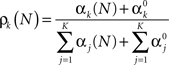
A sample of synthetic RTs and model fit (for the optimal model) over one block for one subject is shown in Figure 2A. Figure 2B shows the estimated probability of τ from which we read the most probable value to be four past events (the decay function for which is shown in Figure 2C). Critically, the results concur with the known true value from which the data were generated.

FIGURE 2

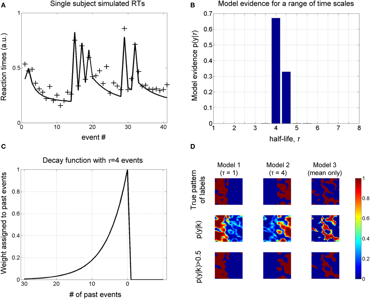
Figure 2. Simulations. (A) A sample of simulated RT data from a single subject over one block is shown, along with the model fit (for the most probable half-life, see next figure). (B) The object of estimation is to quantify evidence for a range of half-life values. The model evidence, given RT data, shows an optimum for τ = 4, which concurs with the true value, i.e., that used to generate these data. (C) The most probable decay function over past events is shown, whose value is characteristically halved with every four events into the past. (D) Simulation of spatial data. A square region is partitioned into three areas (labels), corresponding to three different generative models. Data are generated at each pixel depending on the sampled input, u (see Figure 3A), and label assigned to it. The objective is to recover the true pattern of labels, given only these data, i.e., without direct knowledge of the true labels. The true pattern of labels is along the top row, while the estimated probability of belonging to a label is shown below, which is thresholded to give a binary map along the lower row.

We furthermore sought to recover a known spatial pattern of half-lives using BMS maps (Rosa et al., 2010). A square of 32 voxels was partitioned into three regions (or labels), corresponding to three different causes of data sampled from within them: IT indices using a half-life of τ = 1, and τ = 4 and “mean only,” given the same samples from the Bernoulli process above. The true spatial pattern of labels is shown in the upper row of Figure 2D and time series data were generated in each pixel according to which of the three models it belonged.

The evidence for each model is shown in the middle row of Figure 2D, which is thresholded to give a binary map below. We get an impression of how good the method is at measuring the spatial distribution of labels by comparing the upper and lower rows, i.e., true and estimated spatial pattern of labels. As shown in Figure 2D, there is a high correspondence between these maps, suggesting that our approach can recover the true spatial pattern of labels.

We note that it is a current standard of practice to smooth log-evidence maps for each model to increase signal to noise. A consequence of this is that the extent of the “mean only” model reduces as the width of smoothing kernel increases. This is important as it motivates not to include the “mean only” model when analyzing fMRI data, and use a more realistic “null” model comprised of trial onsets and mean.

Reaction Times and fMRI Data

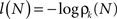
A sample of RTs from one subject over one block of the forced-choice task, including model fit (for the most probable model), and distribution of model evidence over time scales are shown in Figures 3B,C. These are noisy data compared to simulations, which is reflected in the broader distribution of model evidence. However, there is clear evidence for an optimal half-life of four past events. This is important because it concurs with our prediction that there should be evidence for an optimal behavioral time scale of response. This is made all the more striking given the noise inherent in RT data.

FIGURE 3

Figure 3. Reaction time (RT), functional fMRI data, and model evidence. (A) Generative model of the process leading to a measured response, e.g., RT or fMRI data. Each node defines a random variable and arrows connecting nodes signify dependence. A sample from a random process, u, is used to construct IT indices, given a known half-life, and included in a design matrix used to generate data from a GLM. (B) RT data from a single subject over one experimental block along with model fit (for the optimal half-life). (C) Model evidence for the decay half-life for RT data. The greatest support, given the data, was found for τ = 4. (D) Exceedance probability maps (EPM) of fMRI data reveal regions where the greatest evidence for each of the two IT models (model 2: τ = 1; model 3: τ = 4) was observed (short time scale, STS model along the top). In line with theoretical accounts, evidence for short time scales was predominantly in primary and secondary visual cortex (cross hairs centrered on coordinate [0, −79, 4] MNI space) and superior parietal cortex. In addition, we found evidence for this in anterior prefrontal cortex (coordinates, [0, 50, 7]), whereas the largest evidence for long time scales was found in orbitofrontal cortex (coordinates, [6, 38, −14]). Both regions are color coded and shown in greater detail in (E). (E) Overlay of EPMs for both STS and LTS, illustrating the partitioning of prefrontal cortex according to progressively longer time scales. (F) A histogram of the EPM from the voxel containing the maximal value from both regions in (E) are shown on the far right, along with the expected probability to its left.

For the fMRI data, we used the resulting log-evidence maps to quantify the relative evidence for each model, at each voxel. This latter map is an example of a posterior probability map (PPM), which is used in a similar way to statistical parametric maps (SPMs), i.e., to interrogate data. Exceedance probability maps (EPM; STS model along the top) for our computational fMRI analysis are shown in Figure 3D (displayed for illustrative purposes at thresholds of 0.9 and 0.6 for the STS and LTS models, respectively). These are maps showing which model best explains data at each voxel. Figure 3E shows the location of both STS and LTS responses in the frontal cortex, which demonstrates its partitioning into short and LTS regions in line with proposals of a hierarchical organization in this region (Badre, 2008; Kiebel et al., 2008). The expected and exceedance probability at the voxel marked by the cross-hairs (see caption for coordinates) are shown in Figure 3F. This latter quantity is the probability that the k-th model is better than the others.

The “onsets” model did not explain any voxels above a 0.5 threshold. Greatest evidence for the STS model was measured in primary and secondary visual, parietal, and frontal cortices, while that for the LTS model was focused on the frontal cortices. This is striking in that it is in line with the intuitive arguments and predictions made by Kiebel et al. (2008), and supports the notion of a gradient in the scale of time from back to frontal brain regions.

Discussion

The aim of this study was to explore the effect past observations have on human brain responses to uncertainty conveyed by events. It is based on generalizing the computational model used in previous studies (Strange et al., 2005; Harrison et al., 2006; Bestmann et al., 2008; Mars et al., 2008) to depend on a decay function, which we have chosen to be an exponential characterized by its half-life, over past observations. This idea appeals to intuition, in that discarding information from the past is a common human experience. Current neuroscientific theories suggest a temporal gradient within the prefrontal cortex (Badre, 2008) and possibly beyond to include primary sensory and association areas (Kiebel et al., 2008, 2009), and here we provide evidence from functional neuroimaging data that supports this idea.

We have applied this to RT and fMRI data using a Bayesian framework to quantify evidence for the half-life underlying these responses. The optimal half-life observed in behavioral data measured during the experimental task was four past observations. Therefore, no matter how many samples are presented, observers have a threshold on the effective number of past observations that guide their behavior. This provides evidence that observers discount distant information when making inference about statistical regularities in their environment. This, however, is in the context of the current experimental task as one can imagine salient events of a general task that could have an impact on behavior that extend further into the past. The optimal behavioral half-life was then used to inform a group analysis of fMRI data to investigate the multiple neuronal scales that sub-serve it. Given this, we chose to explore two temporal scales, with half-lives of one (STS) and four samples (LTS). While the former appeals to intuition in representing the sensory input of events, the latter was found to be optimal for explaining our behavioral responses to the events. In addition, we predicted that IT indices at these two scales would find greatest evidence in primary visual and frontal regions (involved in controlling executive function) respectively, based on the predictions made by Kiebel et al. (2008). We observed these predictions in fMRI data from 12 subjects along with strong evidence for STS model in the frontal cortex. This latter response is of particular interest because it aligns with the suggestion regarding multiple temporal scales being represented in frontal cortex (Badre, 2008), and that more rostral regions of prefrontal cortex encode more distal time intervals (Fuster, 2004). Other proposals have argued that more complex temporal relationships are represented in more anterior prefrontal regions (Hyafil et al., 2009) and that the temporal scale is the critical parameter that distinguishes the hierarchical organization of the prefrontal lobe (Botvinick, 2008). Consequently, as behavior is governed by temporal regularities, the organization of prefrontal cortex can be explained by the increasing ability to guide behavior based on increasing levels of temporal abstraction. The concordance between prediction and observations found in the present paper provides support for these proposals. More generally, it supports the use of ideas from probability and information theory to investigate the functional architecture of representing uncertainty in the human brain.

Whilst in this paper we have focussed on computing IT indices of sensory events, the same indices can be used to compute, e.g., the amount of information required to decide upon an action (Koechlin et al., 2003). Indeed, because our paradigm employs a one to one deterministic mapping from sensory event to action (i.e., specific visual symbols were mapped onto specific actions) the information required for an action is entirely contained within the stimulus. This corresponds to a situation in which actions are entirely under “sensory control” (Koechlin and Summerfield, 2007) and the action entropy is equal to the sensory entropy. Thus our conclusions about time scales are also relevant to actions.

In order to address the central question of our study, namely the representation of temporal scales in the human brain, we have used an experimental paradigm that is designed to be analyzed using a computational model of brain function. That is, given the assumption that an observer represents uncertainty in data much like a Bayesian statistician, i.e., by estimating probabilities of a causal model that could have generated data, we have chosen a paradigm that depends on a well defined random process, i.e., a Markov process. As such, standard statistical methods to represent this uncertainty (e.g., Bayesian inference with Multinomial likelihoods and Dirichlet priors) can be used. Predicted responses of an observer are then functions of this causal model, of which IT indices are natural candidates. This is because these quantities have meaning in terms of the information contained in data that impacts on an observer, which we know from early experiments goes some way to mapping uncertainty onto behavioral responses (Hick, 1952; Hyman, 1953). These ideas have motivated more recent work using a MD computational model and IT indices to interpret behavioral and neuronal data (Harrison et al., 2006; Bestmann et al., 2008; Brodersen et al., 2008; Mars et al., 2008). While these studies represent an advance, the computational model on which they are based is incapable of investigating the effect of time scales, which is needed to explore the hypothesis that the brain represents causes in the world at multiple temporal scales, as we have done here. We note that the discounting of past observations may vary considerably with the structure and affordances of a task. Future work may address the boundaries over which information is optimally integrated, and whether such boundaries can be shaped by the current context. For example, the complexity of the structure underlying sensory events, or the predictability of the time of occurrence of events may additionally interact with how observers weight past observations.

In terms of the relation of the computational model described here and in other work, an alternative predictor of response to IT indices is to sequentially update the relative entropy between prior and posterior densities (Itti and Baldi, 2009; Baldi and Itti, 2010). Here, we have studied the integration of previous events using a kernel that exponentially weighted previous events. We note that it is also possible to examine the time scale of future events. This can be instantiated from a modeling perspective using a Gaussian kernel that extends over past and future samples, instead of just past events (Lebanon et al., 2007; Mao et al., 2007). This non-causal model may in the future prove a useful tool to measure the multiscale dynamics subserving auditory recognition and our use of natural language. One might also consider the use of asymmetric kernels to fractionate integrative versus predictive processing.

In this paper we compared models using a Bayesian instead of a classical method, i.e., BMS maps instead of F-contrasts. The two are related, but the Bayesian approach is much more general in that one can compare more than two models simultaneously and the models are not restricted to being nested (i.e., one being a special case of another; Rosa et al., 2010). This was useful here because we compared three models; “onsets only,” LTS, and STS models. We envisage that this BMS approach will be of great use more generally in computational fMRI (Corrado and Doya, 2007; O’Doherty et al., 2007; Mars et al., 2010) and that this will allow brain imaging data to directly distinguish between the representations underlying computational models in for example, value updating (Wunderlich et al., 2009), reinforcement learning (Glascher et al., 2010), and perceptual decision making (Forstmann et al., 2010).

Conclusion

We used computational fMRI along with BMS to show how different temporal scales are represented in the human brain. We relax the assumption of an ideal Bayesian observer, by making the integration of past observations dependent on a decay function over past events. Our analysis suggests that forgetfulness, at the level of cortical responses, is possibly a natural consequence reflecting temporal scales within our environment that impact on human behavior.

Conflict of Interest Statement

The authors declare that the research was conducted in the absence of any commercial or financial relationships that could be construed as a potential conflict of interest.

Acknowledgments

We are very grateful to the Medical Research Council (MRC) and Biotechnology and Biological Sciences Research Council (BBSRC) for supporting this work.

References

Badre, D. (2008). Cognitive control, hierarchy, and the rostro-caudal organization of the frontal lobes. Trends Cogn. Sci. (Regul. Ed.) 12, 193–200.

Pubmed Abstract | Pubmed Full Text

Baldi, P., and Itti, L. (2010). Of bits and wows: a Bayesian theory of surprise with applications to attention. Neural Netw. 23, 649–666.

Pubmed Abstract | Pubmed Full Text | CrossRef Full Text

Bestmann, S., Harrison, L. M., Blankenburg, F., Mars, R. B., Haggard, P., Friston, K., and Rothwell, J. C. (2008). Influence of uncertainty and surprise on human corticospinal excitability during preparation for action. Curr. Biol. 18, 775–780.

Pubmed Abstract | Pubmed Full Text | CrossRef Full Text

Bishop, C. (2006). Pattern Recognition for Machine Learning. New York: Springer.

Botvinick, M. M. (2008). Hierarchical models of behavior and prefrontal function. Trends Cogn. Sci. (Regul. Ed.) 12, 201–208.

Pubmed Abstract | Pubmed Full Text

Brodersen, K. H., Penny, W. D., Harrison, L. M., Daunizeau, J., Ruff, C. C., Duzel, E., Friston, K. J., and Stephan, K. E. (2008). Integrated Bayesian models of learning and decision making for saccadic eye movements. Neural Netw. 21, 1247–1260.

Pubmed Abstract | Pubmed Full Text | CrossRef Full Text

Corrado, G., and Doya, K. (2007). Understanding neural coding through the model-based analysis of decision making. J. Neurosci. 27, 8178–8180.

Pubmed Abstract | Pubmed Full Text | CrossRef Full Text

Forstmann, B. U., Brown, S., Dutilh, G., Neumann, J., and Wagenmakers, E. J. (2010). The neural substrate of prior information in perceptual decision making: a model-based analysis. Front. Hum. Neurosci. 4:40. doi: 10.3389/fnhum.2010.00040

Pubmed Abstract | Pubmed Full Text | CrossRef Full Text

Friston, K., and Dolan, R. J. (2010). Computational and dynamic models in neuroimaging. Neuroimage 52, 752–765.

Pubmed Abstract | Pubmed Full Text | CrossRef Full Text

Fuster, J. M. (2001). The prefrontal cortex – an update: time is of the essence. Neuron 30, 319–333.

Pubmed Abstract | Pubmed Full Text | CrossRef Full Text

Fuster, J. M. (2004). Upper processing stages of the perception-action cycle. Trends Cogn. Sci. (Regul. Ed.) 8, 143–145.

Pubmed Abstract | Pubmed Full Text

Glascher, J., Daw, N., Dayan, P., and O’Doherty, J. P. (2010). States versus rewards: dissociable neural prediction error signals underlying model-based and model-free reinforcement learning. Neuron 66, 585–595.

Pubmed Abstract | Pubmed Full Text | CrossRef Full Text

Harrison, L. M., Duggins, A., and Friston, K. J. (2006). Encoding uncertainty in the hippocampus. Neural Netw. 19, 535–546.

Pubmed Abstract | Pubmed Full Text | CrossRef Full Text

Harrison, L. M., Penny, W. D., Flandin, G., Ruff, C. C., Weiskopf, N., and Friston, K. (2008). Graph-partitioned spatial priors for functional magnetic resonance images. Neuroimage 43, 694–707.

Pubmed Abstract | Pubmed Full Text | CrossRef Full Text

Hick, W. E. (1952). On the rate of gain of information. Q. J. Exp. Psychol. 4, 11–26.

CrossRef Full Text

Hyafil, A., Summerfield, C., and Koechlin, E. (2009). Two mechanisms for task switching in the prefrontal cortex. J. Neurosci. 29, 5135–5142.

Pubmed Abstract | Pubmed Full Text | CrossRef Full Text

Hyman, R. (1953). Stimulus information as a determinant of reaction time. J. Exp. Psychol. 45, 188–196.

Pubmed Abstract | Pubmed Full Text | CrossRef Full Text

Itti, L., and Baldi, P. (2009). Bayesian surprise attracts human attention. Vision Res. 49, 1295–1306.

Pubmed Abstract | Pubmed Full Text | CrossRef Full Text

Lebanon, G., Mao, Y., and Dillon, J. (2007). The locally weighted bag of words framework for document representation. J. Mach. Learn. Res. 8, 2405–2441.

Kiebel, S. J., Daunizeau, J., and Friston, K. J. (2008). A hierarchy of time-scales and the brain. PLoS Comput. Biol. 4, e1000209. doi: 10.1371/journal.pcbi.1000209

Pubmed Abstract | Pubmed Full Text | CrossRef Full Text

Kiebel, S. J., Daunizeau, J., and Friston, K. J. (2009). Perception and hierarchical dynamics. Front. Neuroinformatics 3:20. doi: 10.3389/neuro.11.020.2009.

Pubmed Abstract | Pubmed Full Text | CrossRef Full Text

Koechlin, E., and Hyafil, A. (2007). Anterior prefrontal function and the limits of human decision-making. Science 318, 594–598.

Pubmed Abstract | Pubmed Full Text | CrossRef Full Text

Koechlin, E., Ody, C., and Kouneiher, F. (2003). The architecture of cognitive control in the human prefrontal cortex. Science 302, 1181–1185.

Pubmed Abstract | Pubmed Full Text | CrossRef Full Text

Koechlin, E., and Summerfield, C. (2007). An information theoretical approach to prefrontal executive function. Trends Cogn. Sci. (Regul. Ed.) 11, 229–235.

Pubmed Abstract | Pubmed Full Text

Mao, Y., Dillon, J. V., and Lebanon, G. (2007). Sequential document visualization. IEEE Trans. Vis. Comput. Graph 13, 1208–1215.

Pubmed Abstract | Pubmed Full Text | CrossRef Full Text

Mars, R., Debener, S., Gladwin, T. E., Harrison, L. M., Haggard, P., Rothwell, J. C., and Bestmann, S. (2008). Trial-by-trial fluctuations in the event-related electroencephalogram reflect dynamic changes in the degree of surprise. J. Neurosci. 28, 12539–12545.

Pubmed Abstract | Pubmed Full Text | CrossRef Full Text

Mars, R. B., Shea, N. J., Kolling, N., and Rushworth, M. F. (2010). Model-based analyses: promises, pitfalls, and example applications to the study of cognitive control. Q. J. Exp. Psychol. 1–16.

CrossRef Full Text

O’Doherty, J. P., Hampton, A., and Kim, H. (2007). Model-based fMRI and its application to reward learning and decision making. Ann. N. Y. Acad. Sci. 1104, 35–53.

Pubmed Abstract | Pubmed Full Text | CrossRef Full Text

Penny, W., Kilner, J., and Blankenburg, F. (2007). Robust Bayesian general linear models. Neuroimage 36, 661–671.

Pubmed Abstract | Pubmed Full Text | CrossRef Full Text

Penny, W. D., Trujillo-Barreto, N. J., and Friston, K. J. (2005). Bayesian fMRI time series analysis with spatial priors. Neuroimage 24, 350–362.

Pubmed Abstract | Pubmed Full Text | CrossRef Full Text

Rosa, M. J., Bestmann, S., Harrison, L., and Penny, W. (2010). Bayesian model selection maps for group studies. Neuroimage 49, 217–224.

Pubmed Abstract | Pubmed Full Text | CrossRef Full Text

Stephan, K. E., Penny, W. D., Daunizeau, J., Moran, R. J., and Friston, K. J. (2009). Bayesian model selection for group studies. Neuroimage 46, 1004–1017.

Pubmed Abstract | Pubmed Full Text | CrossRef Full Text

Strange, B. A., Duggins, A., Penny, W., Dolan, R. J., and Friston, K. J. (2005). Information theory, novelty and hippocampal responses: unpredicted or unpredictable? Neural Netw. 18, 225–230.

Pubmed Abstract | Pubmed Full Text | CrossRef Full Text

Wunderlich, K., Rangel, A., and O’Doherty, J. P. (2009). Neural computations underlying action-based decision making in the human brain. Proc. Natl. Acad. Sci. U.S.A. 106, 17199–17204.

Pubmed Abstract | Pubmed Full Text | CrossRef Full Text