Sample Entropy, Univariate, and Multivariate Multi-Scale Entropy in Comparison with Classical Postural Sway Parameters in Young Healthy Adults

Introduction

Postural control is of paramount importance to ensure safe completion of complex tasks such as locomotion or simpler tasks such as standing. Postural control in healthy subjects is strongly affected by spatial orientation (Isableu et al., 1998) which in turn is based on both vestibulo-proprioceptive and visual cues (Asch and Witkin, 1948). Some subjects show an increased visual dependency (Guerraz et al., 2001) and therefore closing the eyes or introducing distorted visual feedback (e.g., wearing translucent goggles) increases the difficulty of standing tasks (Bronstein, 1986). A diminished postural control may result in a loss of equilibrium and consequently in falling (Carroll and Freedman, 1993; Collins and De Luca, 1993). This diminution may either be due to normal ageing (Pascolo et al., 2005, 2006) or due to a neurodegenerative disorder such as Parkinson's disease (Sabatini, 2000; Duarte and Zatsiorsky, 2001).

Usually, the quantification of postural control is included in clinical assessments but this strongly depends on the technology available. Either the postural control is rated based on clinical rating scales (Bloem et al., 2016) e.g., Tinetti Balance Scale, Rating Scale for Gait Evaluation, or on specific equipment such as force plates (Yamada, 1995; Newell et al., 1997) to measure body sway. The displacement of the center of pressure (COP) (the point of application of the vertical resultant force acting on the body from the supporting surface, dos Santos, 2008) is commonly measured when evaluating the postural control of a person (Carroll and Freedman, 1993; Collins and De Luca, 1993). The COP is highly irregular and non-stationary which has led multiple studies to characterize the functional effects of conditions such as disease, aging, cognitive task and visual perception on the postural stability (Ramdani et al., 2009).

Techniques for quantifying the displacement of the COP vary from descriptive measures (mean or standard deviation) to techniques taken from signal processing (root-mean-square and frequency analyses). The non-linear deterministic methods allow for the exploration of the randomness or predictability of the COP fluctuations. Those methods were used in studies investigating the deterministic features of COP dynamics (Myklebust et al., 1995; Riley et al., 1999; Doyle, 2004; Doyle et al., 2005), and their potentially chaotic behavior (Cavanaugh, 2005; Costa et al., 2005; Roerdink et al., 2006; Cavanaugh et al., 2007) but also on the quantification of the complexity of COP time series (Ramdani et al., 2009). Entropy family, as a non-linear measure of time series, has been widely applied to study features of COP displacement in different situations.

Entropy family quantifies the regularity (predictability) of a signal, with predictable (e.g., periodic) signals resulting in low entropy, or completely unpredictable signals, resulting in high entropy. A more regular COP pattern indicates that the postural behavior is more rigid (Donker et al., 2007), suggesting that the regularity of COP displacements and the amount of attention paid to postural control are dependent (Donker et al., 2007; Vuillerme and Nafati, 2007). Complexity on the other hand is associated with meaningful structural richness (Grassberger, 1991) incorporating correlations over multiple spatio-temporal scales. A decrease of complexity is related with a functional decline; and a more rigid postural behavior results in dysfunctional balance control during perturbations (Schniepp et al., 2013).

For instance, the Sample Entropy (SE) (Roerdink et al., 2006) has been used to investigate the effect of visual perception (Sabatini, 2000), cerebral concussion (Cavanaugh, 2005; Cavanaugh et al., 2007) and cognitive tasks (Wei et al., 2012) on postural dynamics. Multi-scale Entropy (MSE) and Multivariate Multi-Scale Entropy (MMSE) (Ahmed and Mandic, 2011) are both able to represent the complexity of non-linear time series in different scales (Ahmed and Mandic, 2011). They measure and quantify the intrinsic complexity (Costa et al., 2005) of single and multi-channel signals and then provide a meaningful measure of regularity in biological signals as e.g., COP measurements (Ahmed and Mandic, 2012).

To extract additional features of the COP displacement, the analysis of incremented time series of original signals may be useful (Ramdani et al., 2009) and this approach provides extra information compared to other approaches (Huang et al., 2013). Incremented time series, equivalent to the velocity of the COP displacements have been shown to be effective in the analysis of physiological signals (Costa et al., 2007). In this study two types of incremented time series were computed and studied, the relationship between anterior-posterior (A/P) and medio-lateral (M/L) COP displacement while using univariate and bivariate entropy measures. Although previous studies (Costa et al., 2007; Ramdani et al., 2009) applied incremental time series in their COP analysis, no proof has been provided to determine its performance and advantage.

The working hypothesis was to test if non-linear entropy family methods quantify COP displacement better when using incremented time series during three standing conditions with varying visuo-kinesthetic input. In addition to the entropy measures, classical posturographic methods were also used to assess the COP displacement. The classical methods were then compared with the entropy measures of the original time series.

Methods Experiments and Subjects

Eleven healthy subjects (Mean age: 25.6 years; Mean bodyweight 73.76 kg) voluntarily participated in the experiment after signing a statement of informed consent as required by the Helsinki declaration and the Paris-Saclay STAPS (Sciences and Techniques of Sports and Physical Activities) local Ethics Committee. Subjects stood upright looking forward, on a force plate (AMTI OR6001200, Watertown, MA, USA) with their arms hanging loosely by their sides and feet separated by a self-selected distance (typically approximately 10 cm) for 30 s. Foot position was marked with an erasable marker to ensure the position was maintained if subjects needed to step off the force plate between trials or conditions. Subjects performed three trials of stationary bipedal standing in three different sensory conditions, eyes open (EO), eyes closed (EC) and perturbed vision (PV) by wearing translucent goggles, resulting in a total of nine trials. The trials for each condition were averaged accordingly.

In the PV condition, even though the eyes were opened, the visual input did not constitute a valid and meaningful source (i.e., neither self-motion nor self-orientation cues) of spatial referencing for postural balance, and cannot be integrated together with proprioception in an optimal manner (Jeka et al., 2000; Oie et al., 2001). Conditions were presented in a random order for each participant. Subjects were instructed to stand as still as possible with either the eyes open, eyes closed or wearing translucent goggles. The COP trajectories were recorded in both A/P and M/L directions at a sampling frequency of 250 Hz as shown in Figure 1. Rest periods of 60 s were provided between trials. The resulting data was low-pass filtered at 5 Hz using an 8th order Butterworth filter with a zero-phase digital filter (filtfilt.m) in the Matlab (MathWorks, Inc., USA) environment.

FIGURE 1

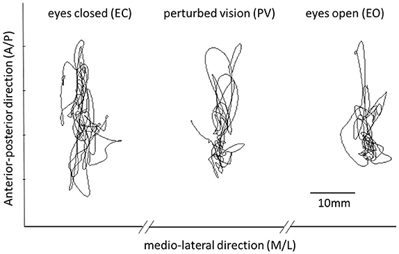
Figure 1. This figure shows representative time series of COP data in each of the three experimental conditions (EO, EC, PV). Differences between conditions are explored using both classical parameters and entropy based methods.

Analysis

Classical Methods

To quantify differences between the conditions (EC, PV, EO), the following variables were calculated from the postural sway: the root-mean square (RMS), mean velocity (MV), path length (PL), mean frequency (MF) and the surface area (SA) of COP displacements in A/P and M/L directions. The RMS was defined as the quadratic mean and is a measure of the postural sway displacement in both the A/P and M/L directions [mm]. The mean velocity defines the mean velocity of the postural sway representing the path length divided by the trial duration [mm/s]. The path length was defined as the length of the COP trajectory displacements on the platform surface [mm]. The MF is the mean frequency of the power spectrum of the postural sway in both the A/P and M/L directions. The SA is the surface area given by the 95% confidence ellipse representing the smallest ellipse that covers 95% of the points of the postural sway [mm²] (Paillard et al., 2006).

Non-linear Methods

Three non-linear methods were used to measure the regularity of COP signals and compare their sensitivity between the incremented time series and the original time series. Sample Entropy is essentially a negative logarithm of conditional probability of the sequences of a data vector. If a vector of length N has repeated itself in tolerance γ for m points, it will also do so for m+1 points. The conditional probability means the ratio of counts of repeated time of m+1 points to that of m points. Thereby, high SE arises from a low probability of repeated sequences in the data. Higher SE means lower regularity and more complexity in the data. On the basis of SE, MSE is a method to evaluate the complexity of signals over different time-scales while MMSE generalizes the analysis to the multivariate case (Wei et al., 2012).

The SE is mathematically computed as follows:

First, from a vector X_N = {x₁, x₂, …, x_N}, two sequences of m consecutive points X_m(i) = {x_i, …, x_i+m−1} and X_m(j) = {x_j, …, x_j+m−1} (i, j ∈ [1, N − m], i ≠ j) are selected to compute the maximum distance and compared to tolerance γ for repeated sequences counting, according to Equation (1). For the sequence X_m(i), its count is defined as ${\mathrm{\text{B}}}_{\mathrm{\text{i}}}^{\mathrm{\text{m}}}(\gamma )$.

$\begin{array}{l}d\left[X_m(i),X_m(j)\right]=\text{max}[\left|x_{i+k},x_{j+k}\right|]\\ \le \gamma (\text{k}\in \left[0,\text{m}-1\right],\gamma \ge 0)& (1)\end{array}$

1 where the tolerance γ equals to 0.1~0.2*SD (Richman and Moorman, 2000), SD is the standard deviation of X_N.

B^m(γ) is the average amount of ${\mathrm{\text{B}}}_{\mathrm{\text{i}}}^{\mathrm{\text{m}}}(\gamma )$ for i ∈ [1, N − m], and B^m+1(γ) is the average of m +1 consecutive points. Thus, SE is obtained using the Equation (2).

$\begin{array}{l}SE(N,m,\gamma )=-ln\left[\frac{B^{m+1}(\gamma )}{B^m(\gamma )}\right]\hfill \\ =-ln\left[\frac{{\left(\text{N}-\text{m}-1\right)}^{-1}{{\displaystyle {\sum }_{\text{i}=1}^{\text{N}-\text{m}-1}\text{B}}}_{\text{i}}^{\text{m}+1}\left(\gamma \right)}{{\left(\text{N}-\text{m}\right)}^{-1}{{\displaystyle {\sum }_{\text{i}=1}^{\text{N}-\text{m}}\text{B}}}_{\text{i}}^{\text{m}}\left(\gamma \right)}\right]& (2)\end{array}$

MSE has a coarse-grain procedure for the data vector X_N before SE computation, which is the main computation difference between MSE and SE. Due to this procedure, MSE is able to measure the distribution of complexity on multiple time-scales, which is fundamentally different from SE. The coarse-grain procedure averages each τ points to generate a new sequence from the data. It is similar to a non-overlapping mean filter with a window length τ. Changing τ leads to sequences in different time-scales. Higher τ means lower frequency components in the sequences. MSE generates the complexity distribution of the data through the sequences in different time-scales, and MSE is equal to SE when τ = 1. The parameter m is the length of repeated mode in the data vector, which is defined by the data itself; and the tolerance γ decides the limitation condition of repeated mode. In biological time-series analysis, m is typically set at 2 or 3 and γ is 0.15*standard deviation (SD) (X_N) (Costa et al., 2005).

To calculate MSE, the following steps have to be computed: the first step is to form a sequence $y_j^{(\tau )}$ based on the scale factor τ, which can be found using the Equation (3):

$\begin{array}{ll}{y}_j^{(\tau )}=\frac{1}{\tau }{\displaystyle {\sum }_{i=(j-1)\tau +1}^{j\tau }}{x}_i& (3)\end{array}$

The equation to compute MSE can be expressed as follows:

$\begin{array}{ll}MSE(N,m,\tau ,\gamma )=-\ln \left[\frac{A^{m+1}(\gamma )}{A^m(\gamma )}\right]& (4)\end{array}$

where both A^m(γ) and A^m+1(γ) are the average repeated amount of two sequences Y_m(i) and Y_{m + 1}(i) [see Equations (1, 2)] to calculate ${\mathrm{\text{B}}}_{\mathrm{\text{i}}}^{\mathrm{\text{m}}}(\gamma )$) and tolerance γ is also for the formed sequences $y_j^{(\tau )}$ with the length N′ = N/τ ∈ [10^m, 30^m] (Pincus and Goldberger, 1994). Therefore, τ is defined by length of N of X_N and m. For example, N = 10,000 and m = 2,500 as the median of [10², 30²] could be selected to calculate the τ_max = 10,000/500 = 20 and τ ∈ [1, 20].

MMSE provides a complexity distribution too, not for a data vector but for the matrix vector from multichannel or multivariate data, which is more adaptive to multi-dimension or multi-parameter time series that are routinely measured in experimental and biological systems.

Given the matrix X(p, N), p is the number of channels or variates, N is the original length, so that the first step for this matrix is just transforming it into a new matrix X′(p, N′), based on scale factor τ regardless of m, which gives the new matrix in a new time scale like the coarse-grain procedure in MSE. In the second step, m and ε are extended to an embedding vector and a time lag vector for a p-variate embedded reconstruction respectively. For the consistence of each variate in the matrix, the values of m and ε are identical, e.g., m = [3,3,3]; ε = [1, 1, 1]. That means three MSE computations with the embedding dimension m = 3 for three variates and the time delay ε = 1. The time delay ε = 1 is the best choice when the minimum embedding dimension for each of the time series is 3 (Cao et al., 1998).

In practice its first step is to define temporal scales of the increased length by coarse-graining the p-variate ${\left\{x_{k,i}\right\}}_{i=1}^N,k=1,2,\dots ,p$. For a scale factor τ, the multivariate coarse-grained time series $y_{k,j}^{(\tau )}$ is calculated [see Equation (5)], where 1 ≤ j ≤ N/τ.

$\begin{array}{ll}{y}_{k,j}^{(\tau )} = \frac{1}{\tau }{\displaystyle \sum _{i = (j - 1)\tau +1}^{j\tau }{x}_{k,i}}& (5)\end{array}$

In order to obtain the MMSE, the multivariate embedded vectors $Y_m(i)\in {ℝ}^p$ must be constructed firstl, which is shown as:

$\begin{array}{l}{Y}_m(i)=[y_{1,i},y_{1,i+{\epsilon }_1},\dots ,y_{1,i+(m_1-1){\epsilon }_1},y_{2,i},y_{2,i+{\epsilon }_2},\dots ,\\ y_{2,i+\left(m_2-1\right){\epsilon }_2},\dots ,y_{p,i},y_{p,i+{\epsilon }_p},\dots ,y_{p,i+\left(m_p-1\right){\epsilon }_p}]& (6)\end{array}$

where $1\le i\le {\mathrm{\text{N}}}^{\prime }-n\mathrm{\text{and}}{\mathrm{\text{N}}}^{\prime }=N/\tau ,n=max\left\{M\right\}\times max\left\{\epsilon \right\}.M=\left[m_1,m_2,\dots ,m_p\right]\in {ℝ}^p$is the embedding vector, while ε = [ε₁, ε₁, …, ε_p] is the time lag vector and $M=\sum _{k=1}^p{m}_k$. Then the maximum norm is defined by Chebyshev distance between any two composite delay vectors Y_m(i) and Y_m(j), that is expressed as:

$\begin{array}{l}d\left[Y_m(i),Y_m(j)\right]=ma{x}_{l=1,\dots ,m}\\ \left\{\left|y\left(i+l-1\right)-y(j+l-1)\right|\right\}& (7)\end{array}$

where j ∈ [1, N′ − n], j ≠ i. For a given Y_m(i), P_i is the number of vector pairs that meets d[Y_m(i), Y_m(j)] ≤ γ, so that $A_i^m(\gamma )=P_i/({\mathrm{\text{N}}}^{\prime }-n-1)$, where n = max{M} × max{τ}. And for all i, $A^m(\gamma )={({\mathrm{\text{N}}}^{\prime }-n)}^{-1}{\sum }_{i=1}^{{\mathrm{\text{N}}}^{\prime }-n}{A}_i^m(\gamma )$.

Finally, the average similarity A^m(γ) over all i ∈ [1, N′ − n] and the A^m+1(γ) over all i ∈ [1, p * (N′ − n)] are used to gain the MMSE, as shown in Equation (8).

$\begin{array}{ll}MMSE(N\prime ,M,\tau ,\gamma )=-ln\left[\frac{A^{m+1}(\gamma )}{A^m(\gamma )}\right]& (8)\end{array}$

where γ is the tolerance level and N′ is the length of the time series $y_{k,j}^{(\tau )}$.

The embedding vector $M=\left[m_1,m_2,\dots ,m_p\right]\in {ℝ}^p$ and the tolerance level γ in MMSE have the equivalent values with parameters m and γ in MSE (Wei et al., 2012).

The three non-linear entropy methods are effective to measure complexity of time series, specifically the SE for the univariate vector, MSE for the univariate vector in multiple time-scale, and MMSE for the multivariate matrix in multiple time-scale respectively. Moreover, it is crucial to have the original time series filtered as all entropy methods are extremely sensitive to random noise. Therefore, our COP data was filtered by a low-pass filter before the computation of entropy.

Incremental Time Series

The postural sway was analyzed in the A/P and the M/L direction, COP (A/P) and COP (M/L) respectively. Additional to the original COP data, its increments were calculated 2-fold: First Δ_incx = [x(t + 1) − x(t − 1)], defined as the Increment; second Δ_diffx = [x(t + 1) − x(t)], defined as Difference. Since mean velocity is a classical parameter of COP estimation, the increments of original COP data, as its equivalent velocity, were created from the original data to remove long-range correlations and avoid potential masking of the complexity of the COP time series.

Simulation

In the simulation, both the original and incremental time series are used to evaluate differences by means of SE, MSE, and MMSE. White noise and 1/f noise are prominent signals to test entropy family measures because of their short-term and long-term correlated properties (Richman and Moorman, 2000; Costa et al., 2005; Ahmed and Mandic, 2011; Wei et al., 2012). To illustrate the behavior of incremental time series and its influence on entropy measures, we considered six time series with a length of N = 20,000 (meeting the range minimum ${10}^m\times {\tau }_{max}$ when m = 3 and τ_max = 20) of each data vector corresponding to 80 s (near to the sum of 30 s in trail and 60 s in rest) of data acquisition at 250 Hz: 1/f noise, 1/f noise Increment, 1/f noise Difference, white noise, white noise Increment, white noise Difference. Increment and Difference are computed from both the 1/f noise and the white noise data through Δ_incx = [x(t + 1) − x(t − 1)] and Δ_diffx = [x(t + 1) − x(t)] respectively. MSE and MMSE were calculated with m = 2 and 3, γ = 0.15*SD (Costa et al., 2005) and a scale factor of τ = 1 to 20 (Figure 2) (meeting the range minimum, Richman and Moorman, 2000).

FIGURE 2

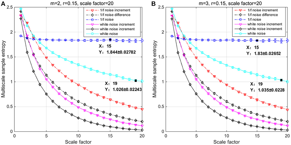
Figure 2. Multiscale entropy (MSE) analysis of white noise, 1/f noise and their Increment and Difference using (A) m = 2, r = 0.15, and τ = 20 and (B) m = 3, r = 0.15, and τ = 20. Each channel has 20 000 data points, and the plots represent an average of 20 independent groups and error bars the standard deviation (SD).

The results of the simulations show decreasing complexity with increasing scale factor except for the 1/f noise series. To understand the differences between m = 2 & 3 on the entropy values, Table 1 shows individual differences as a function of the scale factor for the six considered time series. The simulation results show differences between scale factors 11 and 15 with an absolute deviation of 0.01, indicating that SE is more sensitive on a larger scale with a pattern length of m = 3 (Figure 2). The MMSE analysis of bivariate time series shows similar patterns but larger entropy values in the correlated bivariate time series (Figure 3). When computing MSE and MMSE for short-term correlated signals (white noise), a reduction in complexity occurs with larger scale factors in contrast to long-term correlated signals (1/f noise).

TABLE 1

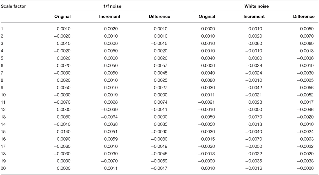
Table 1. Differences between the SE calculated with m = 2 and m = 3 for different scales and noises.

FIGURE 3

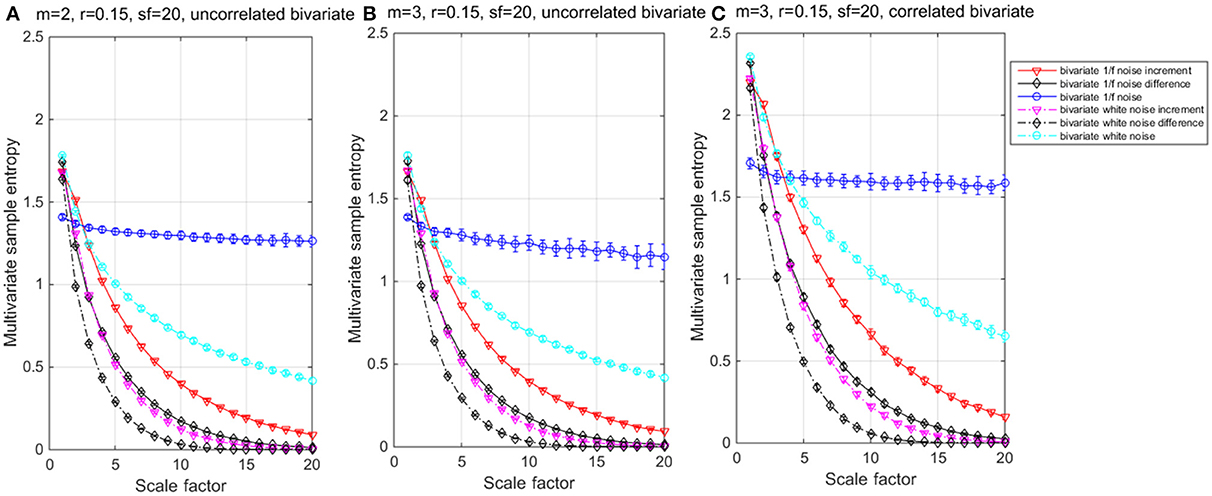
Figure 3. Multivariate multiscale entropy (MMSE) analysis for uncorrelated bivariate 1/f noise, white noise and their Increment and Difference within m = 2 (A) and 3 (B) respectively; and for (C) correlated bivariate 1/f noise, white noise and their Increment and Difference within m = 3.

When computing MSE and MMSE for incremented time series with white noise and 1/f noise, reductions of complexity with increasing scales occur. The incremental time series removes the long-term correlated components from the original time series and represent short-term complexity. Compared to the MSE, the MMSE analysis shows lower entropy values per scale and seems to detect signal divergence faster and can, therefore, be considered more suitable for complexity detection.

Based on the simulation results indicating that SE is more sensitive on larger scales, while m was set to three, γ = 0.15*SD and a scale factor ranging from 1 to 20. A larger scale factor provides a higher resolution of complexity in the time domain and visuo-vestibular regulation is related to low frequencies (0–0.5 Hz) of the COP displacement (Dichgans et al., 1976; Paillard et al., 2006).

Statistical Analysis

Friedman tests were used to examine the effect of condition (i.e., EO, EC, PV) on all postural parameters. The complexity index (CI), defined as the integral of the MSE or MMSE curve, was used for the statistical analysis of the entropy measures (MSE, MMSE). The normality of the data sets was verified using the Kolmogorov-Smirnov test. Post-hoc pairwise comparisons (between-conditions) were performed when needed using Wilcoxon's tests with a Bonferroni adjustment. The effect size values were described by the magnitude of change expressed as Cliff's delta (|r|). All tests were performed using IBM SPSS Statistics version 16 with a level of significance set at p < 0.05.

Results

The Kolmogorov-Smirnov tests indicated non-parametric distribution of the data sets and therefore the data is reported using median (Med) and inter-quartile range (IQR). For the classical parameters, Friedman tests indicated significant differences in path length, mean velocity and mean frequency (A/P), depending on the condition (Table 2). The post-hoc Wilcoxon's analyses revealed a statistically significant difference between the EO and EC conditions for path length, [EC (Med = 230.95, IQR = 120.52) and EO (Med = 184.19, IQR = 53.62), z = 2.934, p ≤ 0.01], mean velocity [EC (Med = 7.7, IQR = 4.02) and EO (Med = 6.14, IQR = 1.78), z = 2.934, p ≤ 0.01], and mean frequency [EC (Med = 0.52, IQR = 0.31) and EO (Med = 0.45, IQR = 0.30), z = 2.934, p ≤ 0.01]. The small effect size calculation for the tree parameters with Cliff's delta values (r < 0.35) suggests minimal practical significance. For the 95% confidence ellipse, mean frequency (M/L), root-mean-square in A/P, or M/L direction (Table 2) no differences were found.

TABLE 2

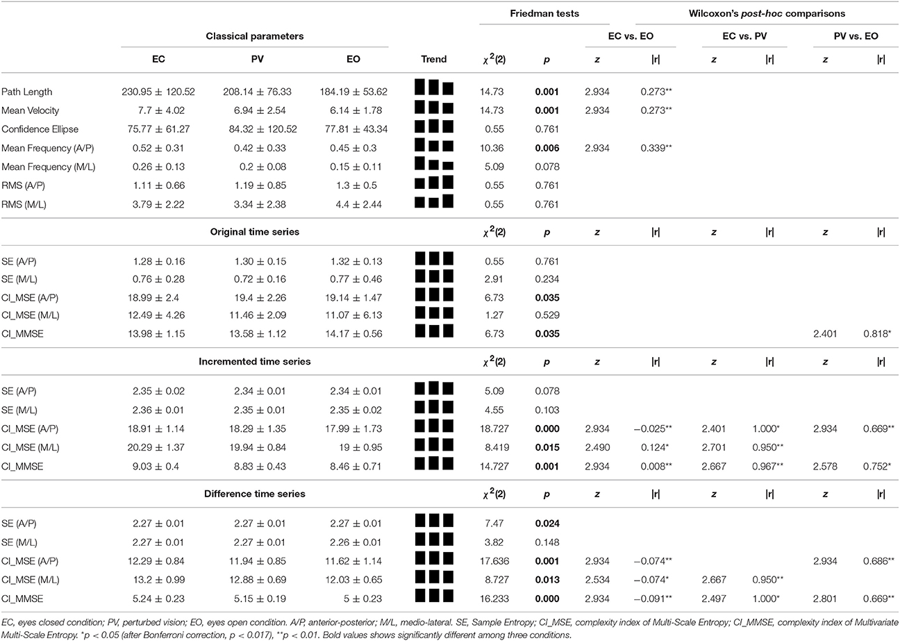
Table 2. Results of non-parametric statistical tests (median ± IQR) on differences between the three experimental conditions (EC, PV, EO) on classical and non-linear complexity parameters.

The analysis for Original time series showed a significant effect of condition on CI_MSE (A/P) and CI_MMSE (Table 2). The post-hoc Wilcoxon's analyses revealed a statistically significant difference between the EO and PV conditions for CI_MMSE, [EO (Med = 13.98, IQR = 1.15) and PV (Med = 13.58, IQR = 1.12), z = 2.401, p ≤ 0.05]. The large effect size calculation with a Cliff's delta value (r > 0.80) suggests high practical significance.

For the Incremented time series, significant differences between conditions were found in three of the five parameters (Table 2). The post-hoc Wilcoxon's analyses revealed a statistically significant difference between the EC and EO conditions for CI_MSE (A/P) [EC (Med = 18.91, IQR = 1.14) and EO (Med = 17.99, IQR = 1.73), z = 2.934, p ≤ 0.01], CI_MSE (M/L) [EC (Med = 20.29, IQR = 1.37) and EO (Med = 19.00, IQR = 0.95), z = 2.490, p ≤ 0.05], and CI_MMSE [EC (Med = 9.03, IQR = 0.40) and EO (Med = 8.46, IQR = 0.71), z = 2.934, p ≤ 0.01]. The small effect size calculation for the tree parameters with Cliff's delta values (r < 0.35) suggests minimal practical significance.

When comparing the EC and PV conditions, the post-hoc Wilcoxon's analyses revealed a statistically significant differences for CI_MSE (A/P) [EC (Med = 18.91, IQR = 1.14) and PV (Med = 18.29, IQR = 1.35), z = 2.401, p ≤ 0.05], CI_MSE (M/L) [EC (Med = 20.29, IQR = 1.37) and PV (Med = 19.94, IQR = 0.84), z = 2.701, p ≤ 0.01], and CI_MMSE [EC (Med = 9.03, IQR = 0.40) and PV (Med = 8.83, IQR = 0.43), z = 2.667, p ≤ 0.01]. The large effect size calculation for the three parameters with Cliff's delta values (r > 0.95) suggests large practical significance.

When comparing the PV and EO conditions, the post-hoc Wilcoxon's analyses revealed statistically significant differences for CI_MSE(A/P) [PV (Med = 18.29, IQR = 1.35) and EO (Med = 17.99, IQR = 1.73), z = 2.934, p ≤ 0.01], and CI_MMSE [PV (Med = 7.7, IQR = 4.02) and EO (Med = 6.14, IQR = 1.78), z = 2.578, p ≤ 0.05]. The medium effect size calculation for the two parameters with Cliff's delta values (r > 0.65) suggests high practical significance.

In the Difference time series, four of the five non-linear parameters significantly changed between conditions (Table 1). The post-hoc Wilcoxon's analyses revealed statistically significant differences between the EO and EC conditions for CI_MSE (A/P) [EC (Med = 12, 29 IQR = 0.84) and EO (Med = 11.62, IQR = 1.14), z = 2.934, p ≤ 0.01], CI_MSE (M/L) [EC (Med = 13.20, IQR = 0.99) and EO (Med = 12.03, IQR = 0.65), z = 2.534, p ≤ 0.05], and CI_MMSE [EC (Med = 5.24, IQR = 0.23) and EO (Med = 5.00, IQR = 0.23), z = 2.934, p ≤ 0.01]. The small effect size calculation for the tree parameters with Cliff's delta values (r < 0.35) suggests minimal practical significance.

When comparing the EC and PV conditions, the post-hoc Wilcoxon's analyses revealed a statistically significant differences for CI_MSE (M/L), [EC (Med = 13.20, IQR = 0.99) and PV (Med = 12.88 IQR = 0.69), z = 2.667, p ≤ 0.01], and CI_MMSE [EC (Med = 5.24, IQR = 0.23) and PV (Med = 5.15, IQR = 0.19), z = 2.497, p ≤ 0.05]. The large effect size calculation for the three parameters with Cliff's delta values (r > 0.90) suggests large practical significance.

When comparing the PV and EO conditions, the post-hoc Wilcoxon's analyses revealed statistically significant differences for CI_MSE (A/P), [PV (Med = 11.94, IQR = 0.85) and EO (Med = 11.62, IQR = 1.14), z = 2.934, p ≤ 0.01], and CI_MMSE [PV (Med = 5.15, IQR = 0.19) and EO (Med = 5.00, IQR = 0.23), z = 2.801, p ≤ 0.01]. The medium to large effect size calculation for the two parameters with Cliff's delta values (r > 0.60) suggests large practical significance.

Discussion

In this experiment, classical parameters were tested against non-linear complexity parameters to reveal differences between the COP displacements during three standing conditions. Non-linear entropy family methods resulted in better uncovering of postural displacement differences when compared to the classical posturographic methods. Only three of the seven classical parameters [i.e., PL, MV, MF (A/P)] were able to differentiate between conditions (EO, EC, PV). Amongst the five studied entropy measures, only two showed significant differences between conditions [i.e., CI_MSE (A/P) and CI_MMSE] using the Original time series, and in the Incremented and Difference time series CI_MSE (A/P), CI_MSE (M/L) and CI_MMSE showed higher sensitivity to the condition effect. Between-conditions differences in the Original time series were only revealed for the CI_MMSE parameter. In the Increment and Difference time series between-conditions differences were found for CI_MSE (A/P), CI_MSE (M/L) and CI_MMSE parameters. The most consistent parameter for the three time series is the CI_MMSE and could therefore be considered as the most reliable parameter in detecting between-conditions differences.

For visual feedback, the results show that the complexity quantified by MSE, and MMSE statistic in Increment and Difference is lower in the EC condition compared to EO and PV. Even though the statistical analysis has not shown significant differences on the COP displacement related to the effect of visual feedback, the entropy values for SE (A/P) of the Original is lowest in the EC condition. Higher entropy values are related to more irregularity, something that may be associated with a functional decline of the postural control system resulting in maladaptive responses to perturbations and thereby destabilizing the balance control (Vaillancourt and Newell, 2002; Schniepp et al., 2013). This finding is consistent with previous research (Roerdink et al., 2011) showing that physical and physiological visual parameters affect postural control during quiet standing and therefore the COP displacement (cf. Stins et al., 2009; Vuillerme and Pinsault, 2009). The sample size and the choice of young healthy participants that were recruited from the Sports Science department may have influenced the results as they may have higher postural capacities compared to age matched subjects. Working with healthy young adults increases the difficulty to distinguish between EO and EC compared to older adults (Prieto et al., 1996). Taking this into account the relation between COP regularity and the amount of attention invested in posture (Donker et al., 2007; Stins et al., 2009), are in line with the findings of our study. The COP regularity in the Original time series showed no differences between conditions by means of sample entropy while in the Difference time series such differences were uncovered. This confirms previous work showing that a decrease of the complexity of the physiological and behavioral systems is observed when the kinesthetic cues are reduced (Newell et al., 1997) but also that incremented time series provide short-term correlated components containing more information about the non-linear system (Ramdani et al., 2009).

Using entropy measures allows us to deal with highly irregular and variable signals like postural sway (Prieto et al., 1996). However, limitations of the particular parameters and properties of the entropy measures have to be discussed. MSE is an entropy measure for univariate time series and MMSE is extended to multivariate cases. Even though the results of MSE and multivariate MSE analysis are promising, some problems still have to be resolved when working with postural data. Entropy measures assess the complexity of physiological time series signals rather than measure motor performance. The creation of one complexity index summing all twenty scales needs to be addressed in future research as it is currently unknown which time-scale is more important or related to postural control. Data length affects entropy measures but it depends on the experiment and therefore a high sampling rate of 250 Hz was chosen to obtain the necessary data length. The COP signal does not contain high frequency signals and the use of a low-pass filter (cut-off 5 Hz) is common. This may create an oversampling issue and the first several scales may not have physiological meaningful information related to dynamical COP changes. Furthermore, the coarse-graining procedure reduced the input data length to half its original size for each successive data scale and therefore potentially changed the intrinsic dynamical scales defined by the signal-generating system.

The reduction of MSE with increasing time-scale is based on the tolerance settings (i.e., constant fraction of the variance of the original time series) and the conventional γ*SD tolerance could be replaced by the variance of each coarse grained time series (Humeau-Heurtier, 2015).

Previous research from our laboratory has shown those MSE characteristics and a possible solution could be the use of diverse empirical mode decomposition techniques (Shih et al., 2015). Decomposing the Original time series into intrinsic mode functions when testing different combinations of frequency bands with relevant complexity indexes has been shown to be efficient and promising in studies on elderly subjects exposed to slight vibrations under their feet (Wei et al., 2012). Empirical mode decomposition and Hilbert–Huang transformation can also be used to observe the physiological signals in instantaneous frequency and instantaneous amplitude through intrinsic mode functions, and then transformed inversely into the time domain to observe the changes in different conditions (Shih et al., 2015). However, the Increment and Difference time series approaches also seem appropriate as they removed trends from the original time series and showed changes in the COP displacements. Other approaches (Yeh et al., 2016) such as the above-mentioned empirical mode decomposition also provide useful data-driven scale factor and intrinsic entropy calculation of complex time series showing the possibility to explore the dynamical complexity of postural control in the future by combining incremented time series and empirical mode decomposition methods.

Conclusions

The current work supports the notion that some measures of non-linear entropy discriminate postural displacement better than classical measures when using incremented time series. Future studies should look to extend applied methods by examining other populations with impaired motor control. We also suggest that future research should consider empirical mode decomposition in combination with incremented time series across different clinical conditions to establish the reliability and validity of this new approach.

Author Contributions

CH, LM, PF, and BI designed and conducted the experiment, QW and JS conducted the analysis and simulations, CH, QW, and JS wrote the manuscript.

Conflict of Interest Statement

The authors declare that the research was conducted in the absence of any commercial or financial relationships that could be construed as a potential conflict of interest.

Acknowledgments

This research was supported by the Innovation Center for Big Data and Digital Convergence, Yuan Ze University, Taoyuan, Chung-Li, Taiwan which is sponsored by Ministry of Education. Also, it was supported by Ministry of Science and Technology (Grant Number: NSC 102-2221-E-155-028-MY3).

References

Ahmed, M. U., and Mandic, D. P. (2011). Multivariate multiscale entropy: a tool for complexity analysis of multichannel data. Phys. Rev. E Stat. Nonlin. Soft Matter Phys. 84(6 Pt 1):061918. doi: 10.1103/physreve.84.061918

PubMed Abstract | CrossRef Full Text | Google Scholar

Ahmed, M. U., and Mandic, D. P. (2012). Multivariate multiscale entropy analysis. IEEE Signal. Process. Lett. 19, 91–94. doi: 10.1109/LSP.2011.2180713

CrossRef Full Text | Google Scholar

Asch, S. E., and Witkin, H. A. (1948). Studies in space orientation. II. Perception of the upright with displaced visual fields and with body tilted. J. Exp. Psychol. 38, 455–475. doi: 10.1037/h0054121

PubMed Abstract | CrossRef Full Text | Google Scholar

Bloem, B. R., Marinus, J., Almeida, Q., Dibble, L., Nieuwboer, A., Post, B., et al. (2016). Measurement instruments to assess posture, gait, and balance in Parkinson's disease: critique and recommendations. Mov. Disord. 31, 1342–1355. doi: 10.1002/mds.26572

PubMed Abstract | CrossRef Full Text | Google Scholar

Bronstein, A. M. (1986). Suppression of visually evoked postural responses. Exp. Brain Res. 63, 655–658. doi: 10.1007/bf00237488

PubMed Abstract | CrossRef Full Text | Google Scholar

Cao, L. Y., Mees, A., and Judd, K. (1998). Dynamics from multivariate time series. Phys. D. Nonlin. Phenomena 121, 75–88. doi: 10.1016/S0167-2789(98)00151-1

CrossRef Full Text | Google Scholar

Carroll, J. P., and Freedman, W. (1993). Nonstationary properties of postural sway. J. Biomech. 26, 409–416. doi: 10.1016/0021-9290(93)90004-X

PubMed Abstract | CrossRef Full Text | Google Scholar

Cavanaugh, J. T. (2005). Detecting altered postural control after cerebral concussion in athletes with normal postural stability. Br. J. Sports Med. 39, 805–811. doi: 10.1136/bjsm.2004.015909

PubMed Abstract | CrossRef Full Text | Google Scholar

Cavanaugh, J. T., Mercer, V. S., and Stergiou, N. (2007). Approximate entropy detects the effect of a secondary cognitive task on postural control in healthy young adults: a methodological report. J. Neuroeng. Rehabil. 4:42. doi: 10.1186/1743-0003-4-42

PubMed Abstract | CrossRef Full Text | Google Scholar

Collins, J. J., and De Luca, C. J. (1993). Open-loop and closed-loop control of posture: a random-walk analysis of center-of-pressure trajectories. Exp. Brain Res. 95, 308–318. doi: 10.1007/BF00229788

PubMed Abstract | CrossRef Full Text | Google Scholar

Costa, M., Goldberger, A. L., and Peng, C. K. (2005). Multiscale entropy analysis of biological signals. Phys. Rev. E 71:021906. doi: 10.1103/physreve.71.021906

PubMed Abstract | CrossRef Full Text | Google Scholar

Costa, M., Priplata, A. A., Lipsitz, L. A., Wu, Z., Huang, N. E., Goldberger, A. L., et al. (2007). Noise and poise: enhancement of postural complexity in the elderly with a stochastic-resonance–based therapy. Europhys. Lett. 77:68008. doi: 10.1209/0295-5075/77/68008

PubMed Abstract | CrossRef Full Text | Google Scholar

Dichgans, J., Mauritz, K. H., Allum, J. H., and Brandt, T. (1976). Postural sway in normals and atactic patients: analysis of the stabilising and destabilizing effects of vision. Agressologie 17, 15–24.

PubMed Abstract | Google Scholar

Donker, S. F., Roerdink, M., Greven, A. J., and Beek, P. J. (2007). Regularity of center-of-pressure trajectories depends on the amount of attention invested in postural control. Exp. Brain Res. 181, 1–11. doi: 10.1007/s00221-007-0905-4

PubMed Abstract | CrossRef Full Text | Google Scholar

dos Santos, A. D. (2008). Multi-muscle Coordination in Postural Tasks. ProQuest Dissertations & Theses Global, 304508614.

Doyle, T. L. A. (2004). Discriminating between elderly and young using a fractal dimension analysis of centre of pressure. Int. J. Med. Sci. 11, 11–20. doi: 10.7150/ijms.1.11

CrossRef Full Text | Google Scholar

Doyle, T. L., Newton, R. U., and Burnett, A. F. (2005). Reliability of traditional and fractal dimension measures of quiet stance center of pressure in young, healthy people. Arch. Phys. Med. Rehabil. 86, 2034–2040. doi: 10.1016/j.apmr.2005.05.014

PubMed Abstract | CrossRef Full Text | Google Scholar

Duarte, M., and Zatsiorsky, V. M. (2001). Long-range correlations in human standing. Phys. Lett. A 283, 124–128. doi: 10.1016/S0375-9601(01)00188-8

CrossRef Full Text | Google Scholar

Grassberger, P. (1991). “Information and complexity measures in dynamical systems,” Information Dynamics, eds H. Atmanspacher and H. Scheingraber (New York, NY: Plenum Press), 15–33.

Google Scholar

Guerraz, M., Yardley, L., Bertholon, P., Pollak, L., Rudge, P., Gresty, M. A., et al. (2001). Visual vertigo: symptom assessment, spatial orientation and postural control. Brain 124, 1646–1656. doi: 10.1093/brain/124.8.1646

PubMed Abstract | CrossRef Full Text | Google Scholar

Huang, L., Zhuang, J., and Zhang, Y. (2013). The application of computer musculoskeletal modeling and simulation to investigate compressive tibiofemoral force and muscle functions in obese children. Comput. Math. Methods Med. 2013, 1–10. doi: 10.1155/2013/698395

PubMed Abstract | CrossRef Full Text | Google Scholar

Humeau-Heurtier, A. (2015). The multiscale entropy algorithm and its variants: a review. Entropy 17, 3110–3123. doi: 10.3390/e17053110

CrossRef Full Text | Google Scholar

Isableu, B., Ohlmann, T., Cremieux, J., and Amblard, B. (1998). How dynamic visual field dependence-independence interacts with the visual contribution to postural control. Hum. Mov. Sci. 17, 367–391. doi: 10.1016/S0167-9457(98)00005-0

CrossRef Full Text | Google Scholar

Jeka, J., Oie, K. S., and Kiemel, T. (2000). Multisensory information for human postural control: integrating touch and vision. Exp. Brain Res. 134, 107–125. doi: 10.1007/s002210000412

PubMed Abstract | CrossRef Full Text

Myklebust, J. B., Prieto, T., and Myklebust, B. (1995). Evaluation of nonlinear dynamics in postural steadiness time series. Ann. Biomed. Eng. 23, 711–719. doi: 10.1007/BF02584470

PubMed Abstract | CrossRef Full Text | Google Scholar

Newell, K. M., Slobounov, S. M., Slobounova, E. S., and Molenaar, P. C. M. (1997). Stochastic processes in postural center-of-pressure profiles. Exp. Brain Res. 113, 158–164. doi: 10.1007/BF02454152

PubMed Abstract | CrossRef Full Text | Google Scholar

Oie, K. S., Kiemel, T., and Jeka, J. J. (2001). Human multisensory fusion of vision and touch: detecting non-linearity with small changes in the sensory environment. Neurosci. Lett. 315, 113–116. doi: 10.1016/S0304-3940(01)02348-5

PubMed Abstract | CrossRef Full Text | Google Scholar

Paillard, T., Noe, F., Riviere, T., Marion, V., Montoya, R., and Dupui, P. (2006). Postural performance and strategy in the unipedal stance of soccer players at different levels of competition. J. Athl. Train. 41, 172–176.

PubMed Abstract | Google Scholar

Pascolo, P., Barazza, F., and Carniel, R. (2006). Considerations on the application of the chaos paradigm to describe the postural sway. Chaos Solitons Fractals 27, 1339–1346. doi: 10.1016/j.chaos.2005.04.111

CrossRef Full Text | Google Scholar

Pascolo, P. B., Marini, A., Carniel, R., and Barazza, F. (2005). Posture as a chaotic system and an application to the Parkinson's disease. Chaos Solitons Fractals 24, 1343–1346. doi: 10.1016/j.chaos.2004.09.062

CrossRef Full Text | Google Scholar

Pincus, S. M., and Goldberger, A. L. (1994). Physiological time-series analysis: what does regularity quantify? Am. J. Physiol. Heart Circ. Physiol. 266, 1643–1656.

PubMed Abstract | Google Scholar

Prieto, T. E., Myklebust, J. B., Hoffmann, R. G., Lovett, E. G., and Myklebust, B. M. (1996). Measures of postural steadiness: differences between healthy young and elderly adults. IEEE Trans. Biomed. Eng. 43, 956–966. doi: 10.1109/10.532130

PubMed Abstract | CrossRef Full Text | Google Scholar

Ramdani, S., Seigle, B., Lagarde, J., Bouchara, F., and Bernard, P. L. (2009). On the use of sample entropy to analyze human postural sway data. Med. Eng. Phys. 31, 1023–1031. doi: 10.1016/j.medengphy.2009.06.004

PubMed Abstract | CrossRef Full Text | Google Scholar

Richman, J., and Moorman, J. (2000). Physiological time series analysis using approximate entropy and sample entropy. Am. J. Physiol. 278, H2039–H2049.

PubMed Abstract | Google Scholar

Riley, M., Balasubramaniam, R., and Turvey, M. (1999). Recurrence quantification analysis of postural fluctuations. Gait Posture 9, 65–78. doi: 10.1016/S0966-6362(98)00044-7

PubMed Abstract | CrossRef Full Text | Google Scholar

Roerdink, M., De Haart, M., Daffertshofer, A., Donker, S. F., Geurts, A. C. H., and Beek, P. J. (2006). Dynamical structure of center-of-pressure trajectories in patients recovering from stroke. Exp. Brain Res. 174, 256–269. doi: 10.1007/s00221-006-0441-7

PubMed Abstract | CrossRef Full Text | Google Scholar

Roerdink, M., Hlavackova, P., and Vuillerme, N. (2011). Center-of-pressure regularity as a marker for attentional investment in postural control: a comparison between sitting and standing postures. Hum. Mov. Sci. 30, 203–212. doi: 10.1016/j.humov.2010.04.005

PubMed Abstract | CrossRef Full Text | Google Scholar

Sabatini, A. M. (2000). Analysis of postural sway using entropy measures of signal complexity. Med. Biol. Eng. Comput. 38, 617–624. doi: 10.1007/BF02344866

PubMed Abstract | CrossRef Full Text | Google Scholar

Schniepp, R., Wuehr, M., Pradhan, C., Novozhilov, S., Krafczyk, S., Brandt, T., et al. (2013). Nonlinear variability of body sway in patients with phobic postural vertigo. Front. Neurol. 4:115. doi: 10.3389/fneur.2013.00115

PubMed Abstract | CrossRef Full Text | Google Scholar

Shih, M.-T., Doctor, F., Fan, S.-Z., Jen, K.-K., and Shieh, J.-S. (2015). Instantaneous 3D EEG signal analysis based on empirical mode decomposition and the hilbert–huang transform applied to depth of anaesthesia. Entropy 17, 928–949. doi: 10.3390/e17030928

CrossRef Full Text | Google Scholar

Stins, J. F., Michielsen, M. E., Roerdink, M., and Beek, P. J. (2009). Sway regularity reflects attentional involvement in postural control: effects of expertise, vision and cognition. Gait Posture 30, 106–109. doi: 10.1016/j.gaitpost.2009.04.001

PubMed Abstract | CrossRef Full Text | Google Scholar

Vaillancourt, D. E., and Newell, K. M. (2002). Changing complexity in human behavior and physiology through aging and disease. Neurobiol. Aging 23, 1–11. doi: 10.1016/S0197-4580(01)00247-0

PubMed Abstract | CrossRef Full Text | Google Scholar

Vuillerme, N., and Nafati, G. (2007). How attentional focus on body sway affects postural control during quiet standing. Psychol. Res. 71, 192–200. doi: 10.1007/s00426-005-0018-2

PubMed Abstract | CrossRef Full Text | Google Scholar

Vuillerme, N., and Pinsault, N. (2009). Experimental neck muscle pain impairs standing balance in humans. Exp. Brain Res. 192, 723–729. doi: 10.1007/s00221-008-1639-7

PubMed Abstract | CrossRef Full Text | Google Scholar

Wei, Q., Liu, D. H., Wang, K. H., Liu, Q., Abbod, M., Jiang, B., et al. (2012). Multivariate multiscale entropy applied to center of pressure signals analysis: an effect of vibration stimulation of shoes. Entropy 14, 2157–2172. doi: 10.3390/e14112157

CrossRef Full Text | Google Scholar

Yamada, N. (1995). Chaotic swaying of the upright posture. Hum. Mov. Sci. 14, 711–726. doi: 10.1016/0167-9457(95)00032-1

CrossRef Full Text | Google Scholar

Yeh, J. R., Peng, C. K., and Huang, N. E. (2016). Scale-dependent intrinsic entropies of complex time series. Philos. Trans. R. Soc. Math. Phys. Eng. Sci. 374:20150204. doi: 10.1098/rsta.2015.0204

PubMed Abstract | CrossRef Full Text | Google Scholar