Integrating temporal and spatial scales: human structural network motifs across age and region of interest size

1 Introduction

The set of connections in the brain can be described as the connectome (Sporns et al., 2005). Connectome data is currently becoming available at different levels of the structural organization: from neuronal networks of connections between neurons to fiber-tract networks between brain regions. These data promise to give valuable new insights, but analyses integrating different data sets are challenging. One problem of data integration across labs is that the raw data might show different voxel resolutions due to different magnetic field strengths of the magnetic resonance imaging (MRI) scanner. In addition, different labs might use different parcelation routines or brain atlases. This leads to different spatial resolutions and consequently to different structural connectivity networks (eventually with different numbers of nodes) (Bassett et al., 2010; Fornito et al., 2010; Hayasaka and Laurienti, 2010; Zalesky et al., 2010). Another problem of data integration is caused by age differences between subjects. There is a certain evidence that characteristics of the connectome vary over age (Fair et al., 2009; Uhlhaas et al., 2009; Fan et al., 2010; Hagmann et al., 2010). Given a network analysis result of two studies, say concerning small-world features (Watts and Strogatz, 1998), are differences due to the study population’s differences in connectivity or are they due to differences in age or network resolution? In this article, we observe how topological and spatial network features change across age and network resolution for structural connectivity, based on diffusion tensor imaging (DTI), in healthy human subjects. Using single node motifs, we also apply a network mapping technique, which yields a compact and easily comparable representation of complex network structures.

1.1 Scales of a Hierarchical Organization

Hierarchy is a central feature in the organization of complex biological systems and particularly the structure and function of neural networks (Kaiser and Hilgetag, 2010; Kaiser et al., 2010). In neural networks, the term hierarchy may be understood in several different ways and can apply to topological, spatial, temporal as well as functional properties. These features can be observed at different scales or resolutions.

1.1.1 Temporal scales

Network analysis is often presented as the analysis of a network at a given time, but many networks change both over time and with temporal resolution. Structural connectivity, given by anatomical connections between neurons or brain regions, may change due to activity-dependent plasticity (Butz et al., 2009). Functional connectivity, given by correlations in the activity patterns of network nodes, can change for different tasks for a subject or due to different system states (e.g., awake vs. asleep). In our case, connectivity might also change over longer time-scales, as part of brain development.

Recovered networks can appear differently depending on temporal resolution. At a fine-grained temporal resolution of a few hundred milliseconds, cortical tissue can show distinct oscillations, e.g., in the α, γ, or δ frequency bands (Roopun et al., 2008). For more coarse-grained time-resolutions with sample lengths of several seconds or minutes such distinct frequency peaks disappear and the frequency distribution displays a 1/f power-law behavior instead (Buzsaki, 2006).

Here, we observe temporal scale in terms of snapshots of structural connectivity at different points in time. The human brain undergoes large structural developments until the age of around 20–25 years. These developments coincide with large functional changes during child development and during the teenager years. They further coincide with changes in functional connectivity (Uhlhaas et al., 2009). Such changes during brain network development are not only of interest for the study of healthy subjects, but also for many psychiatric disorders like schizophrenia (Uhlhaas and Singer, 2010), which have an onset around the time when the brain network matures (age 18–25 years). We therefore test the potential of single node motifs to integrate information across temporal network “snapshots”.

1.1.2 Spatial scales

The network structure not only depends on the time of a “snapshot” but also on the spatial resolution. One can distinguish the micro- and macro-connectome as the connectivity between individual neurons and connections between brain regions, respectively (DeFelipe, 2010). In this study of structural connectivity we focus on the macro-connectome level based on MRI data [see Seung (2009) for more information about neuronal connectivity instead].

The macro-connectome can be analyzed at different levels of spatial resolution and thus different levels of brain network organization. With a low spatial resolution, it corresponds to connectivity between brain areas where network nodes correspond to brain regions. The resulting networks show features of modular and small-world networks (Hilgetag et al., 2000; Sporns et al., 2000) and typically consist of up to 100 nodes per cortical hemisphere for the primate brain. At the mesoscale, connectivity between regions of interest (ROIs) of the same size, e.g., 1 cm² cortical surface area, can be studied. Such networks consist of around 1000 nodes for the human brain (Hagmann et al., 2008). With even higher resolution, the microscale of the macro-connectome could be studied, i.e., connections between cortical columns (Mountcastle, 1997). However, such networks with nodes representing one cortical column each would consist of 1,250,000 nodes for the human brain (both hemispheres, not including subcortical structures) and identifying columns with diameters ranging from 200 μm to 1 mm (Hubel et al., 1977; Horton and Adams, 2005) in humans is (currently) beyond the reach of standard MRI. Such extremely high resolutions might only be achieved with higher magnetic fields or extremely high magnetic fields in post mortem studies.

We therefore study the global and regional scale of the macro-connectome. Importantly, this level allows us to assess whether motifs which are characteristic for a certain cortical region are also characteristic for all parts of that cortical area or whether a region displays a variety of motifs at higher spatial resolutions. Also, changes in spatial resolution affect spatial measurements, which form part of the motif detection. It is often interesting to observe how many connections go to nearby targets and how many extend over a long distance, potentially linking different components of the neural network. This can be readily observed using a histogram of the connection lengths of a network. It is known that the probability that two neurons are connected decays almost exponentially with distance (Hellwig, 2000; Schüz et al., 2005; Kaiser et al., 2009): connections over a long distance are less likely than short-distance connections. In different organisms, ranging from neuronal connectivity in C. elegans and layers in the rat visual cortex to fiber-tract connectivity in the macaque, the actual distribution was approximated best by a Gamma probability density function (Kaiser et al., 2009). Looking at different spatial resolutions within humans, we would expect that the proportion of short-distance connections relative to long-distance connections increases when the spatial resolution is increased. We will therefore observe how the length distributions change over different spatial scales.

1.2 Single Node Motifs

Networks can be analyzed following different concepts: to investigate a single network, for example, analysis can focus on its nodes, comparing them through connectional fingerprints based on the absolute values of node properties (e.g., node degree or local clustering coefficient; Passingham et al., 2002). On a more abstract level, nodes of brain networks can be regarded with respect to their different organization levels. These approaches look at one network of a particular subject, but networks can also be compared across different subjects – or different networks might exist for the same subject across time. However, mapping between networks becomes difficult if the number of nodes and edges varies, such that direct comparisons (i.e., link-to-link or node-to-node) between structures are ruled out. In contrast to such methods of cross-comparison, the approach used in this paper is less sensitive to these changes: although a network with a slightly higher number of nodes could show additional motifs, most nodes are non-outliers making such changes less likely. Similarly, a network with slightly more edges might show absolute changes in network features without affecting the outliers of the feature distribution leading to similar single node motifs. Again, these comparisons of the number and classes of motifs become possible for non-identical numbers of nodes or edges but only if the numbers do not differ too much. These motif-classes are significantly different from each other and they allow to classify network nodes at the same level even if they appear in different networks.

The concept of node motifs – a combination of local network features – complements that of network motifs, which are specific connectivity patterns that have been used to characterize networks before (Milo et al., 2002). An example for a node motif are highly connected nodes or hubs that affect spreading phenomena and can be important components of a network. More complex, multi-dimensional node motifs, which are characterized by multiple features in combination, specify nodes more comprehensively. With these more precise descriptions, new kinds of motifs can be formulated and Costa et al. (2009) presented a routine for their detection and specification. We proposed first improvements and procedures for automating parameter choices for this method (Echtermeyer et al., 2011), such that large numbers of networks can be processed and compared to each other. This enhanced technique is applied to brain networks in this paper.

1.3 Comparing Motif Counts Across Networks

The usefulness of mapping brain networks (which itself are abstract representations) to motif-classes is demonstrated for two scenarios: first, regional connectomes of 53 children (aged 12–23 years) are compared to show how the fingerprint of a DTI network can change over time. Second, we test the effect of different connectome-resolutions on the resulting network-fingerprint. Therefore, DTI networks at different levels of organization were generated by changing the level of granularity from 414 ROIs to up to 1615 ROIs.

Comparing networks from the same subject but at different granularities has so far been complicated by the critical dependence of standard approaches on the resolution of the network (Antiqueira et al., 2010). We show how our novel node fingerprints can be used to compare different levels of connectome organization.

Note that comparing motifs has several advantages over comparing network features. Features, such as the small-world measures of clustering coefficient and characteristic path length, critically depend on the edge density of a network. Therefore, changes in these measures could be either due to changes in network organization (e.g., modularity) or due to a difference in the number of connections. To identify the changes related to network organization, the edge density needs to be constant when comparing networks. However, this leads to a severe problem: when transforming raw data of connection strengths between nodes to binary data, each network needs a different threshold for establishing a connection (Rubinov and Sporns, 2010). To avoid the problem of either having different edge densities or different thresholds, researchers increasingly use weighted networks without thresholding (Bullmore and Bassett, 2011). For our analysis, we expect that differences in edge density are not only due to inter-subject variability, as in other studies, but are more heavily influenced by changes across different temporal or spatial scales. Therefore, we observe how network measures, and as a result node motifs, change over scales. These changes can be due to changes in organization or edge density.

Although a detailed analysis is outside the scope of this paper, we show the relation between both scales in Figure 1. Whereas edge density decreases with network size, there are no significant changes between age groups when looking at networks with the same spatial resolution. However, we would like to point out that (a) motifs change over time and can therefore be used to find characteristic changes in the developing brain and (b) motifs change over spatial scales, therefore comparisons between studies are only meaningful when the same (or a comparable) spatial resolution has been used.

FIGURE 1

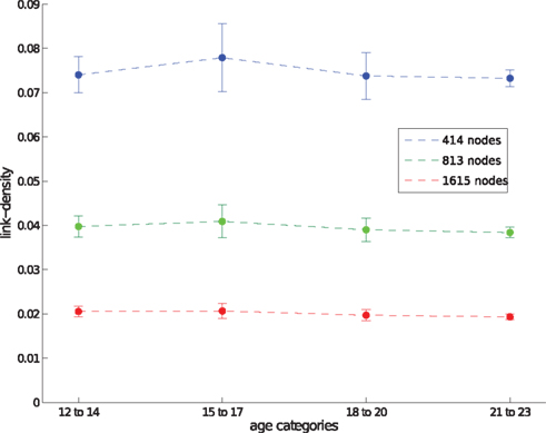
Figure 1. Edge density for different spatial resolutions, given by the number of network nodes, and different age groups. Data points show the average edge density of all networks belonging to a certain age group and spatial resolution. Corresponding SDs are shown by error-bars.

2 Materials and Methods

2.1 Recruiting and Data Recording

We recruited 53 participants (age between 12 and 23 years) from local community and high schools. The study received ethics committee approval and written informed consents were obtained from the participants’ parents for under-age participants, or from themselves if older than 18 years after study procedures were described. Participants were screened for a history of psychiatric and neurological disorders and current drug abuse using ophthalmological assessment including monocular and binocular visual acuity. Participants were grouped into four age-categories (Table 1).

TABLE 1

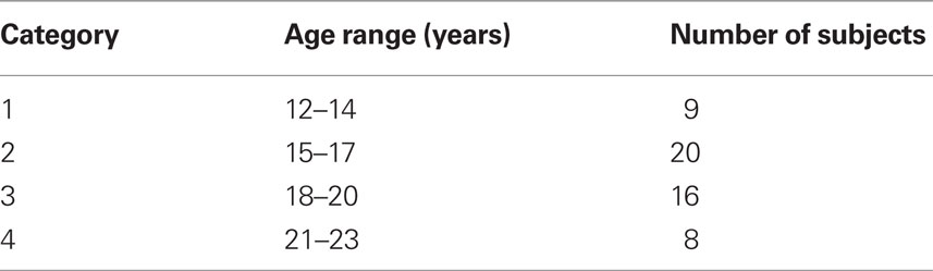
Table 1. Ranges of age-categories.

A 3-Tesla scanner (Siemens Trio, Erlangen, Germany) was used at the Brain Imaging Centre (BIC), Frankfurt am Main, Germany. We recorded T1 weighted MRI (voxel-size 1 mm × 1 mm × 1 mm) and Diffusion Tensor MRI (voxel-size 2 mm × 2 mm × 2 mm). To minimize head motion, we used tightly padded clamps on the eight-channel head coil. The T1 weighted MRI was recorded with the following parameters: 176 slices, field of view (FoV) 256 mm, repetition time (TR) 2250 ms, and echo time (TE) 2.6 ms. Three Diffusion Tensor Images per participant were recorded with the following parameters: 60 slices, FoV 192 mm, TR 7600 ms, TE 91 ms, 60 directions b-vectors with b-factor of 1000 and 10 b0-images.

2.2 Data Processing and Network Construction

We used FreeSurfer to obtain surface meshes of the boundary between gray matter and white matter from T1 anatomical brain images¹, and Diffusion toolkit along with TrackVis (Wang et al., 2007) to obtain stream-line tractography from diffusion tensor images. We registered surface meshes into brains of the diffusion tensor images to extract networks. FreeSurfer provides parcelation of anatomical regions of cortices (33 for each hemisphere) based on the Deskian atlas (Fischl et al., 2004b; Desikan et al., 2006) and subcortices (Fischl et al., 2002, 2004a). We subdivided those anatomical regions of cortices into many of similar surface area using our own algorithm. It is known that the size of each ROI affects network connectivity and various network measures (Hagmann et al., 2007; Zalesky et al., 2010). The core of our algorithm is an expectation–maximization (EM) algorithm. First, we choose the expected number of subdivisions (400, 800, and 1600) for cortical regions (we do not subdivide subcortical areas) and decided the number of subdivisions based on the ratio of each surface area over whole surface area in the average subject. Then we subdivide each anatomical cortical region to the assigned number of subdivisions using the EM algorithm, minimizing variance of subdivisions’ surface area sizes. The ratio of variance to mean does not exceed 10% in the average subject. In each subject, this ratio was higher (400: 414.78 ± 140.06 mm², 33.77%; 799: 207.65 ± 77.51 mm², 37.33%; 1601: 103.63 ± 44.33 mm², 42.78%, statistics of cortical ROIs only) because the size of each subject’s anatomical region varied (2468.06 ± 1813.10 mm², 73.46%, which represents individual subjects’ regions were 12 ± 30% bigger than the average subject’s; ratio of variance to mean is 26.49%). Another useful statistic is the ratio of interquartile range to median: larger values represent higher dispersion. The values (Table 2) are smaller than those determined by Fornito et al. (2010).

TABLE 2

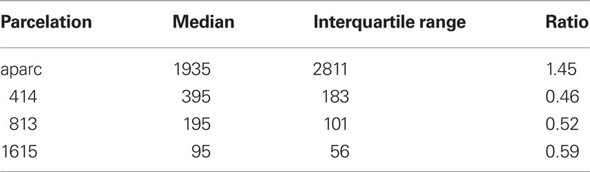
Table 2. Region of interest (ROI) surface area (mm²) statistics with ratio of interquartile range to median.

We projected this new parcelation template into each subject’s surface. Using this projection procedure we kept topological consistency across all subjects. We also included a few selected subcortical areas in the ROI list: nucleus accumbens, Amygdala, Caudate, Hippocampus, Pallidum, Putamen, and Thalamus. Thus the actual number of ROIs (414, 813, and 1615, respectively) is slightly larger than specified. These three numbers of ROIs on the brain and resulting networks are shown in Figure 2. Before further processing the diffusion tensor images, we serialized three diffusion tensor images and b-vectors for each participant; thus, a collated image of each subject has 30 b0-images and 180 diffusion images. The eddy current was corrected through FSL². We used Diffusion toolkit along with TrackVis (Wang et al., 2007) with fiber assignment by continuous tracking (FACT) algorithm (Mori et al., 1999) and 35° of angle threshold. After registering the surface meshes (FreeSurfer³) of each subject to his/her DTI, we generated cortical volume ROIs, which are voxels in the gray matter. Also the selected subcortical areas (see above) were registered to DTIs and used as ROIs. Then, we used the UMCP toolbox⁴ to obtain connectivity matrices from the defined and registered ROIs and tractography. This counts the number of fibers from a tractography from the Diffusion toolkit, between all pairs of defined ROIs’ gray matter; the fiber counts between all ROI-pairs yield the weight-matrix. We also computed the average fiber lengths between ROIs (if there is no connection between a pair, the length is set to zero). The fiber length is based on the actual three-dimensional trajectory of the fiber tract and may be larger than the Euclidean distance between connected nodes. Note that long fiber length usually also corresponds to a large Euclidean distance between ROIs: earlier studies in fiber tracts in primates have shown that 85% of the fibers go in a straight line or are only slightly curved (Hilgetag and Barbas, 2006). However, only a fully bended (U-turn) fiber could result in a long fiber-tract connection to spatially nearby nodes.

FIGURE 2

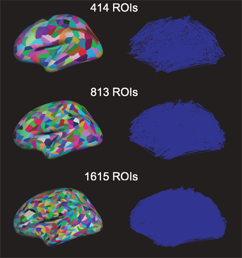
Figure 2. Region of interests (ROIs) on the brain (left) and the resulting networks (right) with different numbers of ROIs.

Diffusion tensor imaging fiber-tracking yielded weighted matrices where weights indicate the probability of connections between corresponding ROIs. Non-zero weights have been interpreted as an indication for a link when constructing the brain networks. The resulting adjacency matrices were similarly sparse for each network resolution (Figure 1, average link-densities 7.5, 4.0, and 2.0% for networks of 414, 813, and 1615 nodes, respectively).

2.3 Network Analysis

Single node motifs were identified from the constructed networks by applying a technique presented by Costa et al. (2009) with additions in order to choose parameters automatically (Echtermeyer et al., 2011). The method yields a global characterization of the network based on its local properties. Here, each node is quantified by nine different local measures, which are motivated in the next paragraph. We chose such a large number of local measures, some of which share similarities, to ensure that as many network features as possible are considered. Redundancies, where two features are highly correlated, are removed during the node-motif detection, which is explained further below.

A nodes’ degree is its number of connections to other nodes; dividing this by the number of all links in the network yields the normalized node degree K. The average over all neighbors’ degrees is called the normalized average degree r. (Nodes that are directly linked to each other are called neighbors.) Degrees of a node’s immediate neighbors can further be taken into account by their respective coefficient of variation cv. Connectivity among neighbors of a node is quantified by the clustering coefficient cc, which reflects how many of all possible connections between neighbors actually exist (Watts and Strogatz, 1998; Kaiser et al., 2007a). The hierarchical clustering coefficient of level two cc₂ extends this concept to connections between neighbors’ neighbors (Costa and Silva, 2006). To what degree a node’s neighbors connect to the same target is quantified by the locality index loc, which is based on the matching index (e.g., Kaiser and Hilgetag, 2004a). The six measures mentioned so far quantify topological aspects of the network, while the next three measures also take into account spatial features. The average connection length acl for a node is the average length of fiber tracts to its neighbors and the furthest away neighbor determines the maximum connection length mcl. The average over connection lengths to nodes two steps away, i.e., neighbors’ neighbors, is called the average indirect reach air. Further details and measures can be found in the literature (Albert and Barabási, 2002; Newman, 2003; Newman et al., 2006; Costa et al., 2007b).

The motif-detection workflow starts by applying the above listed network measures (Figure 3): local network measures are calculated for all nodes of the network, which yields a nine-dimensional characterization (feature vector) for each node. This high-dimensional representation is simplified by exploiting similarities between different measures (Costa et al., 2007b): using principal component analysis (PCA; Johnson and Wichern, 2007, Chapter 8), correlation between measures is removed and the feature vectors are reduced to two dimensions (PCA-plane). The position on the PCA-plane characterizes the nodes and allows for comparisons: nodes close to each other share similar features whereas well separated ones differ. The next step is to estimate how likely specific combinations of features are. This is done by smoothing over points in the PCA-plane using the Parzen window approach (Parzen, 1962; Duda et al., 2001, Chapter 4.3) with width of the smoothing kernel scaled according to the SD along the corresponding principal component axis (Echtermeyer et al., 2011). Thereby, each node is assigned a probability, which is used to distinguish those with common and rare features. The w many nodes with uncommon properties, termed outlier nodes, were determined as follows. Given all nodes’ probabilities p = (p_k)_{k = 1,…, n} (sorted increasingly), the respective mean , and SD σ(p), the number of singular nodes w is chosen as

FIGURE 3

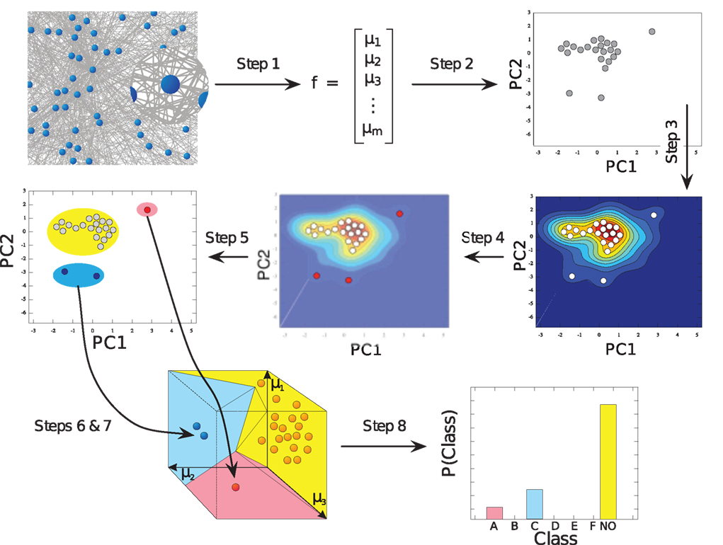
Figure 3. Figure from Echtermeyer et al. (2011). Illustration of network analysis workflow: high-dimensional characterization of all network nodes through local network measures μ_i (Step 1) is compacted to two dimensions (Step 2) in order to estimate a probability distribution (Step 3), which is used to identify nodes with uncommon features (Step 4). All nodes are grouped (Step 5) to form high-dimensional motif-regions (Step 6), which are eventually joined, if too close to each other (Step 7). The number of nodes in each motif-region yields a fingerprint of the network (Step 8).

or w = 0, if all probabilities are greater than Nodes corresponding to the smallest w probabilities are the identified outliers. Next, the outlier nodes were assigned to clusters each of which represents a different motif-group, i.e., a set of features. This was done by first centering equally sized ellipses on each point and determining their overlap. Maximal sets of nodes whose ellipses form a connected area yield both the number k of motif-groups as well as the groups themselves. (The above mentioned mechanisms have been evaluated and discussed in detail in an earlier publication (Echtermeyer et al., 2011).) Motif-groups correspond to nine-dimensional motif-regions in feature space, such that all nodes within a motif-group are similar with respect to the local network measures used in the beginning. In the final step, motif-regions from all networks were reduced to the final nine motif-regions by subsequently joining the closest two of them. The pairwise distances have been determined with a modified Mahalanobis measure (Mahalanobis, 1936). The number of nodes that express a particular motif yields a fingerprint of the network, which characterizes the network and allows for comparisons (Costa et al., 2009), e.g., by considering the motif-diversity, which is the number of unique motifs k that were identified. Another possibility is to compare the number of outlier nodes w.

3 Results

3.1 Motif Changes with Age

Networks were first analyzed with respect to age-dependent changes. Therefore, outlier motifs were determined for all networks to see whether certain motifs might only be expressed in subjects of similar age. This was not the case, but the total number of outlier nodes w shows a characteristic pattern with age (Figure 4, solid blue lines). Subjects of young ages (13–14 years) show 3–4 outlier nodes on average – a number that is reduced throughout the teenager years and thereafter (15–20 years) until a sudden and predominant peak at the age of 21. Subjects aged 22–23 years have again fewer, but still several outlier nodes. This pattern is qualitatively preserved for different network resolutions (Figure 4 top to bottom). Quantitatively, the number of outlier nodes w rises with larger networks.

FIGURE 4

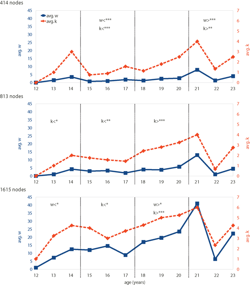
Figure 4. Motif-expression changing with age: both the number of outlier nodes in a network w (solid blue line) and the diversity of motifs expressed k (dashed orange line) vary with subject age. The time-dependent patterns of w and k are shown for different network resolutions (rows). Age groups indicated by dashed vertical lines. Significantly de- or increased values for w and k are indicated by symbols < and >, respectively (*90, **95, and ***99% significance). Note that our data only include one subject aged 21 and further data would be needed to confirm significance of deviations at this age.

To determine which changes are statistically significant a random permutation test has been applied: subjects were randomly assigned an age (12–23 years) while ensuring that each age group had the same size as for the original data. Subsequently, each group’s mean w and k were compared to those of the original data to compute the p-values (using a total of 500,000 permutations). Results, shown directly in Figure 4, represent how far each group is to the average over age. Note that except for the lowest network resolution, the large spike at age 21 does not lead to significant increase in w (and k). This is because our data only include one subject aged 21 and further data would be needed to confirm that the deviations at this age are indeed significant across all scales of resolution.

A pattern that is very similar to that of the outlier number w is the diversity k of expressed motifs. The number k is high and low for nearly the same ages as was the number of outliers w before (Figure 4, dashed orange lines), which is also reflected by the strong correlation between w and k (Pearson correlation 0.94, 0.88, and 0.87 for 414-, 813-, and 1615-node networks, respectively). Peaks at low (13–14 years) and high (21 years) ages can be seen with a dip in between. This pattern fits networks with 414 nodes best, whereas networks with the higher resolution (813 and 1615 nodes) show an increasingly flat profile except for the later peak (21 years). Note that absolute motif-diversity k is relatively similar for all network resolutions, which was not the case for the actual number of outliers w.

Both, number of outliers w and motif-diversity k are interesting on their own, but their strong correlation provides additional information. Although the absolute values differ, similarity of the curves’ profiles is independent of network resolution. We thus find the very robust effect that motif-diversity is coupled to the number of outlier nodes. In other words, whenever more outliers occur, they also become more diverse.

3.2 Motif Changes with Network Resolution

The previous section has already shown that network resolution affects outlier quantity, w, but not the relative distribution across the age range (Figure 4, solid blue lines). Different from that, motif-diversity, i.e., how many different motifs are expressed, k, is nearly invariant on an absolute scale, in contrast to its relative distribution (Figure 4, dashed orange lines). We tested whether the number w and diversity k of outliers, at different spatial scales, are correlated with cognitive skills of our subjects. Unfortunately, measures of intelligence yielded by four sub-scores of the Wechsler intelligence test were only available for 44 out of our 53 subjects. For all comparisons, the Pearson correlation was r ≤ 0.5. Therefore, we cannot confirm a link between intelligence and w or k. However, intelligence might still be related to a specific combination of motifs; a possibility which could only be tested given a larger cohort of subjects. Next, we analyze the actual frequencies with which motifs are expressed by different age groups (Table 1).

Using the same raw DTI-data, networks have been constructed with different resolutions, i.e., differently sized ROIs, for each subject. More fine-grained ROIs parcelate the brain into more elements, each of which is represented by a network node. We were interested in the effect that different network resolutions have on the occurring node motifs (Table 3; Figure 5) and therefore, networks with 414, 813, and 1615 nodes were analyzed and compared to each other.

TABLE 3

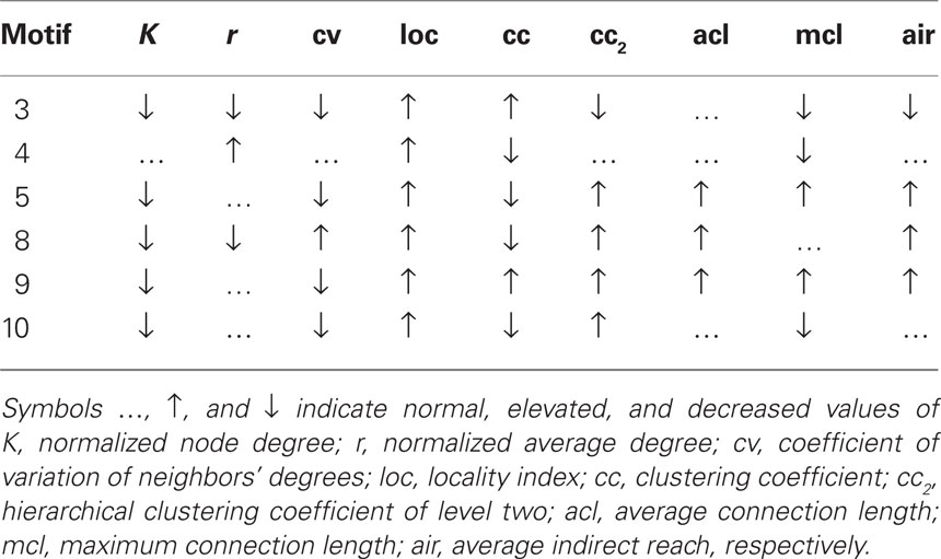
Table 3. Properties of most frequent motifs.

FIGURE 5

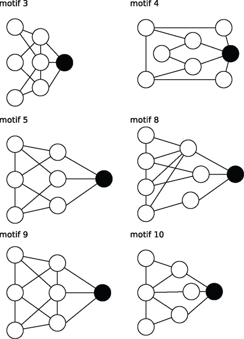
Figure 5. Stylized illustration of most frequent motifs (Table 3): motif 3 Provincial node with connections in the direct (high cc) but not the larger neighborhood (low cc₂, air, and mcl). motif 4 Provincial hub with more connections than its neighbors (high r) that are less connected between themselves (low cc). motif5 Global bottleneck with few (low K) but long-range connections (high acl, mcl, air) that reach beyond the local neighborhood (low cc). motif 8 Global uniform bottleneck sharing properties of motif 5 but connected to nodes with similar degrees (low cv). motif 9 Global local bottleneck sharing properties of motif 5 but also having well-connected neighbors (high cc) thus better informing local circuits. motif 10 Provincial bottleneck with only short-range connections (low mcl) and few connections between its neighbors (low cc) leading to a large influence on the local circuit.

The results show that motif-expression strongly depends on network resolution (Figure 6). Whereas motif 4 is most frequent for the 414-node resolution, it is nearly absent in the highest resolution of 1615 nodes. Other motifs also show large fluctuations between spatial resolutions with either increasing or decreasing frequency. Motifs can also be characteristic for a single scale. For example, motifs 8, 9, and 10 are most prevalent across age groups at an intermediate resolution of 813 nodes. This shows that the spatial resolution is critical for assessing the frequency of motifs and, presumably, also for its underlying spatial and topological features.

FIGURE 6

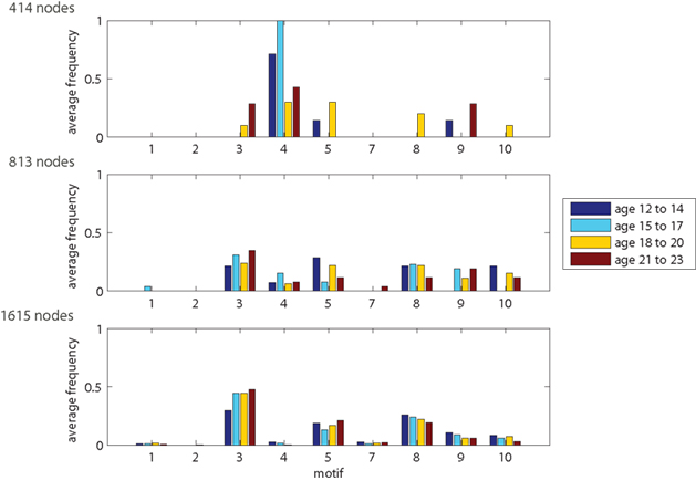
Figure 6. Motif-expression changing with network resolution. Plots show distribution of outlier nodes among motifs 1–5 and 7–10. Motif 6 (not shown) corresponds to the remaining 98% network nodes with common features (regular nodes).

Motif counts also depend on age. For 414-node networks, many motifs only occur for one or two out of the four age groups. Whereas this might be influenced by the low number of nodes in the network, we also see age-based motif frequency changes for higher spatial resolutions. Looking at the resolution of 1615 nodes, the number of nodes showing motifs 3 and 5 increases with age whereas motifs 8 and 9 become less frequent. These age-dependent trends are less visible at 813-node resolution and they disappear for the 414-node networks.

3.3 Fiber Length Distribution for Different Network Sizes

A possible explanation for the observed dependence on network resolution could be fiber length based network measures (namely: average connection length, maximum connection length, and average indirect reach). These measures take into account the determined fiber trajectory between ROIs, i.e., their fiber-tract length. It is thus to be expected that the number of ROIs impacts on the corresponding fiber lengths. We tested this by observing the fiber length distribution for different network resolutions (Figure 7). Across all resolutions, short fibers are more frequent than long fibers. This exponential tail, which can be fitted by a Gamma distribution (Kaiser et al., 2009), has been reported before not only at the level of fiber tracts (Kaiser and Hilgetag, 2004b), but also at the level of connections between neurons within cortical areas (Hellwig, 2000). One notable difference between spatial resolutions is the increase in the number of short fibers (length < 10 mm) increasing by more than 50% from the lowest to the highest spatial resolution. This can be due to the smaller size of network nodes where surface regions that before belonged to the same node are now separate nodes on the surface. Therefore, a short fiber tract between these nodes becomes feasible. Looking at the maximum range of fibers, spatial resolution does not seem to influence maximum fiber lengths. However, differences in average fiber length, in particular due to an increased number of short fiber connections, might occur for particular nodes. The pattern for average indirect reach is more complex and can be influenced by changes in both short and long fibers. Overall, given a three-fold increase in spatial resolution, the fiber length distributions remain remarkably similar.

FIGURE 7

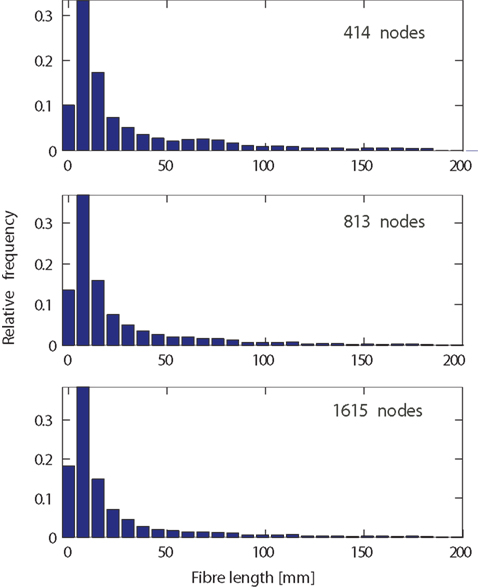
Figure 7. Fiber length distribution, as the length of the trajectory in millimeter, for different network resolutions. Relative frequencies for low (414 nodes, top), medium (813 nodes, middle), and high (1615 nodes, bottom) spatial resolution. Note that longer fibers (>200 mm) occurred so infrequently that corresponding bars (not shown) would be invisible.

3.4 Motif Consistency Across Spatial Scales

How consistent are motifs across different resolutions? If a region splits into several regions for higher resolutions, do the daughter regions show the same motif as the parent region? Interestingly, this does not seem to be the case. Figure 8 shows a typical example of motif locations for one subject. For 414 nodes, one location shows motif 3. One part of this location then shows motif 8 for the resolution of 813 nodes. For 1615 nodes, part of the original region shows motif 3 again, whereas another part shows motif 9. This is an interesting point when talking about the connectivity between brain regions: a pattern shown at the low-resolution level (e.g., cortical regions or Brodmann areas) may consist of several diverse patterns when observing connectivity at a higher resolution.

FIGURE 8

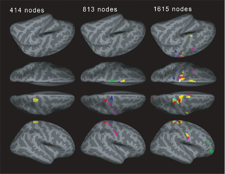
Figure 8. Example for the motif distribution in one subject (19 years old) for different spatial resolutions. Different number of regions of interests (ROIs, left: 414, middle: 813, and right: 1615) with different views: left lateral view, left superior view, right superior view, and right lateral view in order from the top. Yellow: motif 3, magenta: motif 4, cyan: motif 7, red: motif 8, green: motif 9, blue: motif 10 (motifs 1, 2, and 5 were not present).

4 Discussion

We observed how the distribution (fingerprint) of characteristic motifs of single network nodes changed for human structural connectivity (DTI) during brain development. We studied the role of both temporal scales (age groups from 12 to 23 years) and spatial scales (414, 813, and 1615 nodes) and found that, first, the number and diversity of motifs in a network are strongly correlated. Second, comparing different scales, the number and diversity of motifs varied across the temporal (subject age) and spatial (network resolution) scale (with certain motifs only occurring at one spatial scale or for a certain age range). Third, the sub-regions of a node, using a higher spatial resolution, may or may not include the original motif at the lower resolution. Therefore, both the type and localization of motifs differ for different spatial resolutions. This indicates that spatial resolution is crucial when comparing characteristic node fingerprints given by topological and spatial network features. This result is in line with previous studies that observed the role of sampling on brain network properties (Antiqueira et al., 2010) and it additionally shows the influence of the temporal scale.

Networks can be characterized at different levels. Aggregate measures that characterize a network as a whole can be used to distinguish different network types, e.g., small-world (Watts and Strogatz, 1998; Hilgetag et al., 2000; Sporns et al., 2000), scale-free (Eguiluz et al., 2005; Kaiser et al., 2007b), modular (Hilgetag et al., 2000), or hierarchical (Kaiser et al., 2010). Networks can also be characterized at the level of individual components. Looking at the topological features of individual nodes, a first study by Passingham et al. (2002) has linked the network features of macaque cortical areas with the function of each area. Whereas this approach considered all nodes of the network, there are also ways to search for “special” nodes of a system. Following the ideas of scale-free networks, brain areas with a large number of connections – so-called network hubs – might be crucial for integrating or distributing information (Kaiser et al., 2007b). Sporns et al. (2007) were able to detect and classify different kinds of hubs of cortical structural connectivity. However, hubs are just one type of outliers where one or more node features (here: the number of connections of a node) differ from the average value of nodes in the network. In two previous manuscripts (Costa et al., 2009; Echtermeyer et al., 2011), we have developed a tool that systematically searches for and classifies nodes which differ from the majority of nodes in a network. This approach includes the joint analysis of multiple features, which include topological as well as spatial properties (Costa et al., 2007a).

Our measures are based on outliers, which do not show the overall trend as shown in previous studies (spatial resolution dependent changes: Zalesky et al. (2010), Bassett et al. (2010), Fornito et al. (2010), Hayasaka and Laurienti (2010), age-dependent changes: Fan et al. (2010), Hagmann et al. (2010), Fair et al. (2009); Uhlhaas et al. (2009), Table A1 in Appendix). Thus, it is difficult to directly relate our results to their findings. However, our report that edge density decreased with increased spatial resolution is consistent with previous studies of structural connectivity (Bassett et al., 2010; Zalesky et al., 2010). For the temporal resolution, most previous studies showed no overlap with the age range of our study. Hagmann et al. (2010) performed a study with overlapping temporal scales, but only observed ages up to 18 years and thus only about half of the temporal scales considered in our study. Studies with larger overlap focused on functional rather than structural connectivity (Uhlhaas et al., 2009; Fan et al., 2010).

Here we noted that surface areas of used ROIs varied around 33–43% compared to their mean (shown only for the cortical ROIs because subcortical ROIs were not subdivided, Table 2). This variation stems from the variation of anatomical regions’ surface areas (ratio of its SD to its mean is 73.5%). The ratio of interquartile range to median showed comparatively small ROI variation (Fornito et al., 2010). To keep the topological consistency, this might be the best we can do. At least, this is better than using just anatomical regions whose variation is much higher (73.5% variation).

This node fingerprint study is a proof of principle for the current technique showing the influence of spatial and temporal scales on network comparison. However, the current results could also be influenced by the following points. First, the number of subjects per age group was not identical (Table 1). Therefore, findings in age groups with fewer members might have been influenced by relatively few outliers. Whereas an identical number of subjects per group is desirable, for our study there was also a trade-off with the age range: using the same subject numbers would have led to groups where the age ranges differ, e.g., covering 3 years for one group and 5 years for another. We decided for a different number of subjects per group in order to perform the comparison across the temporal scale. Second, single node motifs become more robust for larger network sizes. As node motifs are outliers, only a small percentage of all nodes will be characterized as node motifs. Therefore, for low-resolution networks, node motifs might only occur for few subjects. In addition, their number might be a poor estimate of the underlying frequency in human connectivity networks. For this reason, we have only reported networks with at least 414 nodes, leaving out networks with a parcelation into 110 cortical and subcortical regions. Third, node features but not necessarily motifs depend on the edge density of the network. In our developmental networks, we observed significant edge density changes for different spatial resolutions ranging from more than 7% for 414 nodes to 2% for 1615 nodes. However, for each network resolution, edge densities remained comparable for different temporal scales (age groups; Figure 1). Fourth, deterministic tracking cannot capture crossing fibers which can be done in probabilistic tracking (Behrens et al., 2007), in Diffusion spectrum imaging (Wedeen et al., 2008; Bassett et al., 2010), or in high-angular resolution diffusion imaging (HARDI; Tuch, 2004; Zalesky et al., 2010). However, fiber length distributions, influencing our three spatial features, were similar across resolutions (Figure 7).

Network Science has led to a wide range of tools for analyzing neural systems (Sporns et al., 2004; Costa et al., 2007b; Bullmore and Sporns, 2009; Rubinov and Sporns, 2010; Kaiser, 2011). Whereas the characterization of individual networks, e.g., as small-world or scale-free, is now possible, comparing different networks is still a challenge. Our study shows how node properties, given by characteristic single node motif fingerprints, can be compared between different networks. Studying single node properties is only one way to characterize networks with alternatives being (a) the study of global properties including local and global efficiency (Latora and Marchiori, 2001; Achard and Bullmore, 2007) as well as modularity (Newman, 2006), (b) the comparison of the cluster organization of different networks, and (c) direct comparison of network matrices (Crofts and Higham, 2009). However, it is problematic for these measures that network features are influenced by the number of nodes and edges of a network; feature changes between networks might simply be due to different edge densities in the compared systems (van Wijk et al., 2010). For our networks, edge densities did not significantly differ across age but they differed across spatial resolutions. Whereas the underlying topological and, to some extent, spatial features might have changed in our networks, our motif fingerprints do not depend on the absolute values for network measures but on their distribution: an overall increase or decrease in the average value of a measure will have less of an influence on the number of node motifs as these depend on statistical outliers and not on absolute values of a measure.

Nonetheless, nodes that present characteristic node motifs, as well as hubs, are rare within networks. These fingerprints can therefore only be applied for high-resolution networks (≥414 nodes) and large groups of subjects. Fortunately, large subject cohorts are currently being recruited in several initiatives including the Human Connectome Project for structural connectivity and the 1000 Functional Connectome Project (Biswal et al., 2010). In addition, fingerprints will also be useful for high-resolution networks at the scale of the micro-connectome observing connections between individual neurons (DeFelipe, 2010). Another potential application lies in the analysis of multi-electrode array recordings, which nowadays can record from more than 4000 channels (Sernagor et al., 2010). We therefore made this tool available within the CARMEN initiative⁵ for developing electrophysiology analysis tools (Smith et al., 2007). The tool is also available on our website⁶.

5 Conclusion

In this study we found that (a) node motifs change over time and can therefore be used to find characteristic changes in the developing brain and (b) motifs change over spatial scales, therefore comparisons between studies are only meaningful when the same (or a comparable) spatial resolution has been used. Our results also indicate that spatial resolution has a higher effect on topological measures whereas spatial measures, based on fiber lengths, remain more comparable between resolutions. As node motifs are based on topological and spatial properties of brain connectivity networks, these conclusions are also relevant to other studies using network analysis. Another important aspect is the analysis of differences between healthy controls and subjects with brain disorders that can arise during brain network development, such as schizophrenia and epilepsy; we hope that our node fingerprint approach will be useful for detection and specification in these cases.

Conflict of Interest Statement

The authors declare that the research was conducted in the absence of any commercial or financial relationships that could be construed as a potential conflict of interest.

Acknowledgments

Marcus Kaiser and Christoph Echtermeyer were funded by EPSRC (EP/G03950X/1) and the CARMEN e-science Neuroinformatics project (http://www.carmen.org.uk) funded by EPSRC (EP/E002331/1). Marcus Kaiser and Cheol Han also acknowledge support by the WCU program through the National Research Foundation of Korea funded by the Ministry of Education, Science and Technology (R32-10142).

Footnotes

1. ^http://surfer.nmr.mgh.harvard.edu
2. ^http://www.fmrib.ox.ac.uk/fsl/
3. ^http://surfer.nmr.mgh.harvard.edu/
4. ^http://ccn.ucla.edu/wiki/index.php/UCLA_Multimodal_Connectivity_Package
5. ^http://www.carmen.org.uk
6. ^http://www.biological-networks.org/

References

Achard, S., and Bullmore, E. (2007). Efficiency and cost of economical brain functional networks. PLoS Comput. Biol. 3, e17. doi: 10.1371/journal.pcbi.0030017

Pubmed Abstract | Pubmed Full Text | CrossRef Full Text

Albert, R., and Barabási, A.-L. (2002). Statistical mechanics of complex networks. Rev. Mod. Phys. 74, 47–97.

CrossRef Full Text

Antiqueira, L., Rodrigues, F. A., van Wijk, B. C. M., Costa, L. D. F., and Daffertshofer, A. (2010). Estimating complex cortical networks via surface recordings – a critical note. Neuroimage 53, 439–449.

Pubmed Abstract | Pubmed Full Text | CrossRef Full Text

Bassett, D. S., Brown, J. A., Deshpande, V., Carlson, J. M., and Grafton, S. T. (2010). Conserved and variable architecture of human white matter connectivity. Neuroimage 54, 1262–1279.

Pubmed Abstract | Pubmed Full Text | CrossRef Full Text

Behrens, T. E., Berg, H. J., Jbabdi, S., Rushworth, M. F., and Woolrich, M. W. (2007). Probabilistic diffusion tractography with multiple fibre orientations: what can we gain? Neuroimage 34, 144–155.

Pubmed Abstract | Pubmed Full Text | CrossRef Full Text

Biswal, B. B., Mennes, M., Zuo, X. N., Gohel, S., Kelly, C., Smith, S. M., Beckmann, C. F., Adelstein, J. S., Buckner, R. L., Colcombe, S., Dogonowski, A. M., Ernst, M., Fair, D., Hampson, M., Hoptman, M. J., Hyde, J. S., Kiviniemi, V. J., Kotter, R., Li, S. J., Lin, C. P., Lowe, M. J., Mackay, C., Madden, D. J., Madsen, K. H., Margulies, D. S., Mayberg, H. S., McMahon, K., Monk, C. S., Mostofsky, S. H., Nagel, B. J., Pekar, J. J., Peltier, S. J., Petersen, S. E., Riedl, V., Rombouts, S. A., Rypma, B., Schlaggar, B. L., Schmidt, S., Seidler, R. D., Siegle, G. J., Sorg, C., Teng, G. J., Veijola, J., Villringer, A., Walter, M., Wang, L., Weng, X. C., Whitfield-Gabrieli, S., Williamson, P., Windischberger, C., Zang, Y. F., Zhang, H. Y., Castellanos, F. X., and Milham, M. P. (2010). Toward discovery science of human brain function. Proc. Natl. Acad. Sci. U.S.A. 107, 4734–4739.

Pubmed Abstract | Pubmed Full Text | CrossRef Full Text

Bullmore, E., and Sporns, O. (2009). Complex brain networks: graph theoretical analysis of structural and functional systems. Nat. Rev. Neurosci. 10, 186–198.

Pubmed Abstract | Pubmed Full Text | CrossRef Full Text

Bullmore, E. T., and Bassett, D. S. (2011). Brain graphs: graphical models of the human brain connectome. Annu. Rev. Clin. Psychol. 7, 113–140.

Pubmed Abstract | Pubmed Full Text | CrossRef Full Text

Butz, M., Wörgötter, F., and Van Ooyen, A. (2009). Activity-dependent structural plasticity. Brain Res. Rev. 60, 287–305.

Pubmed Abstract | Pubmed Full Text | CrossRef Full Text

Buzsaki, G. (2006). Rhythms of the Brain. Oxford: Oxford University Press.

Costa, L. D. F., Kaiser, M., and Hilgetag, C. C. (2007a). Predicting the connectivity of primate cortical networks from topological and spatial node properties. BMC Syst. Biol. 1, 16. doi: 10.1186/1752-0509-1-16

CrossRef Full Text

Costa, L. D. F., Rodrigues, F. A., Travieso, G., and Boas, P. R. V. (2007b). Characterization of complex networks: a survey of measurements. Adv. Phys. 56, 167–242.

CrossRef Full Text

Costa, L. D. F., Rodrigues, F. A., Hilgetag, C. C., and Kaiser, M. (2009). Beyond the average: detecting global singular nodes from local features in complex networks. Europhys. Lett. 87, 18008.

CrossRef Full Text

Costa, L. D. F., and Silva, F. N. (2006). Hierarchical characterization of complex networks. J. Stat. Phys. 125, 841–876.

CrossRef Full Text

Crofts, J. J., and Higham, D. J. (2009). A weighted communicability measure applied to complex brain networks. J. R. Soc. Interface 6, 411–414.

Pubmed Abstract | Pubmed Full Text

DeFelipe, J. (2010). From the connectome to the synaptome: an epic love story. Science 330, 1198–1201.

Pubmed Abstract | Pubmed Full Text | CrossRef Full Text

Desikan, R., Se’gonne, F., Fischl, B., Quinn, B., Dickerson, B., Blacker, D., Buckner, R., Dale, A., Maguire, R., Hyman, B., Albert, M., and Killiany, R. (2006). An automated labeling system for subdividing the human cerebral cortex on mri scans into gyral based regions of interest. Neuroimage 31, 968–980.

Pubmed Abstract | Pubmed Full Text | CrossRef Full Text

Duda, R. O., Hart, P. E., and Stork, D. G. (2001). Pattern Classification, 2nd Edn. New York, NY: Wiley Interscience.

Echtermeyer, C., da Fontoura Costa, L., Rodrigues, F. A., and Kaiser, M. (2011). Automatic network fingerprinting through single-node motifs. PLoS ONE 6, e15765. doi: 10.1371/journal.pone.0015765

Pubmed Abstract | Pubmed Full Text | CrossRef Full Text

Eguiluz, V. M., Chialvo, D. R., Cecchi, G. A., Baliki, M., and Apkarian, A. V. (2005). Scale-free brain functional networks. Phys. Rev. Lett. 94, 018102.

Pubmed Abstract | Pubmed Full Text | CrossRef Full Text

Fair, D. A., Cohen, A. L., Power, J. D., Dosenbach, N. U. F., Church, J. A., Miezin, F. M., Schlaggar, B. L., and Petersen, S. E. (2009). Functional brain networks develop from a “local to distributed” organization. PLoS Comput. Biol. 5, e1000381. doi: 10.1371/journal.pcbi.1000381

Pubmed Abstract | Pubmed Full Text | CrossRef Full Text

Fan, Y., Shi, F., Smith, J. K., Lin, W., Gilmore, J. H., and Shen, D. (2010). Brain anatomical networks in early human brain development. Neuroimage 54, 1862–1871.

Pubmed Abstract | Pubmed Full Text | CrossRef Full Text

Fischl, B., Salat, D., Busa, E., Albert, M., Dieterich, M., Haselgrove, C., van der Kouwe, A., Killiany, R., Kennedy, D., Klaveness, S., Montillo, A., Makris, N., Rosen, B., and Dale, A. (2002). Whole brain segmentation: automated labeling of neuroanatomical structures in the human brain. Neuron 33, 341–355.

Pubmed Abstract | Pubmed Full Text | CrossRef Full Text

Fischl, B., Salat, D., van der Kouwe, A., Makris, N., Ségonne, F., Quinn, B., and Dalea, A. (2004a). Sequence-independent segmentation of magnetic resonance images. Neuroimage 23(Suppl. 1), S69–S84.

CrossRef Full Text

Fischl, B., van der Kouwe, A., Destrieux, C., Halgren, E., Ségonne, F., Salat, D., Busa, E., Seidman, L., Goldstein, J., Kennedy, D., Caviness, V., Makris, N., Rosen, B., and Dale, A. (2004b). Automatically parcellating the human cerebral cortex. Cereb. Cortex 14, 11–22.

CrossRef Full Text

Fornito, A., Zalesky, A., and Bullmore, E. T. (2010). Network scaling effects in graph analytic studies of human resting-state fMRI data. Front. Syst. Neurosci. 4:22. doi: 10.3389/fnsys.2010.00022

Pubmed Abstract | Pubmed Full Text | CrossRef Full Text

Hagmann, P., Cammoun, L., Gigandet, X., Meuli, R., Honey, C. J., Wedeen, V. J., and Sporns, O. (2008). Mapping the structural core of human cerebral cortex. PLoS Biol. 6, e159. doi: 10.1371/journal.pbio.0060159

Pubmed Abstract | Pubmed Full Text | CrossRef Full Text

Hagmann, P., Kurant, M., Gigandet, X., Thiran, P., Wedeen, V., Meuli, R., and Thiran, J. (2007). Mapping human whole-brain structural networks with diffusion mri. PLoS ONE 2, e591. doi: 10.1371/journal.pone.0000597

Pubmed Abstract | Pubmed Full Text | CrossRef Full Text

Hagmann, P., Sporns, O. N., Madan Cammoun, L. R., Pienaar Wedeen, V., Meuli, R., Thiran, J., and Grant, P. (2010). White matter maturation reshapes structural connectivity in the alte developing human brain. Proc. Natl. Acad. Sci. U.S.A. 107, 19067–19072.

Pubmed Abstract | Pubmed Full Text | CrossRef Full Text

Hayasaka, S., and Laurienti, P. J. (2010). Comparison of characteristics between region- and voxel-based network analysies in resting-state fmri data. Neuroimage 50, 499–508.

Pubmed Abstract | Pubmed Full Text | CrossRef Full Text

Hellwig, B. (2000). A quantitative analysis of the local connectivity between pyramidal neurons in layers 2/3 of the rat visual cortex. Biol. Cybern. 82, 111–121.

Pubmed Abstract | Pubmed Full Text | CrossRef Full Text

Hilgetag, C. C., and Barbas, H. (2006). Role of mechanical factors in the morphology of the primate cerebral cortex. PLoS Comput. Biol. 2, e22. doi: 10.1371/journal.pcbi.0020022

Pubmed Abstract | Pubmed Full Text | CrossRef Full Text

Hilgetag, C. C., Burns, G. A. P. C., O’Neill, M. A., Scannell, J. W., and Young, M. P. (2000). Anatomical connectivity defines the organization of clusters of cortical areas in the macaque monkey and the cat. Philos. Trans. R. Soc. Lond. B Biol. Sci. 355, 91–110.

Pubmed Abstract | Pubmed Full Text | CrossRef Full Text

Horton, J. C., and Adams, D. L. (2005). The cortical column: a structure without a function. Philos. Trans. R. Soc. B Biol. Sci. 360, 837–862.

CrossRef Full Text

Hubel, D., Wiesel, T., and LeVay, S. (1977). Plasticity of ocular dominance columns in monkey striate cortex. Philos. Trans. R. Soc. Lond. B Biol. Sci. 278, 377–409.

Pubmed Abstract | Pubmed Full Text | CrossRef Full Text

Johnson, R. A., and Wichern, D. W. (2007). Applied Multivariate Statistical Analysis, 6th Edn. Englewood Cliffs, NJ: Prentice Hall.

Kaiser, M. (2011). A tutorial in connectome analysis: topological and spatial features of brain networks. Neuroimage 57, 892–907.

Pubmed Abstract | Pubmed Full Text | CrossRef Full Text

Kaiser, M., Goerner, M., and Hilgetag, C. C. (2007a). Criticality of spreading dynamics in hierarchical cluster networks without inhibition. New J. Phys. 9, 110.

CrossRef Full Text

Kaiser, M., Martin, R., Andras, P., and Young, M. P. (2007b). Simulation of robustness against lesions of cortical networks. Eur. J. Neurosci. 25, 3185–3192.

CrossRef Full Text

Kaiser, M., and Hilgetag, C. C. (2004a). Edge vulnerability in neural and metabolic networks. Biol. Cybern. 90, 311–317.

CrossRef Full Text

Kaiser, M., and Hilgetag, C. C. (2004b). Modelling the development of cortical systems networks. Neurocomputing 58–60, 297–302.

CrossRef Full Text

Kaiser, M., and Hilgetag, C. C. (2010). Optimal hierarchical modular topologies for producing limited sustained activation of neural networks. Front. Neuroinform. 4:8. doi: 10.3389/fninf.2010.00008

Pubmed Abstract | Pubmed Full Text | CrossRef Full Text

Kaiser, M., Hilgetag, C. C., and Kötter, R. (2010). Hierarchy and dynamics of neural networks. Front. Neuroinform. 4:112. doi: 10.3389/fninf.2010.00112

Pubmed Abstract | Pubmed Full Text | CrossRef Full Text

Kaiser, M., Hilgetag, C. C., and van Ooyen, A. (2009). A simple rule for axon outgrowth and synaptic competition generates realistic connection lengths and filling fractions. Cereb. Cortex 19, 3001–3010.

Pubmed Abstract | Pubmed Full Text | CrossRef Full Text

Latora, V., and Marchiori, M. (2001). Efficient behavior of small-world networks. Phys. Rev. Lett. 87, 198701.

Pubmed Abstract | Pubmed Full Text | CrossRef Full Text

Mahalanobis, P. C. (1936). On the generalized distance in statistics. Proc. Indian Natl. Sci. Acad. B Biol. Sci. 2, 49–55.

Milo, R., Shen-Orr, S., Itzkovitz, S., Kashtan, N., Chklovskii, D., and Alon, U. (2002). Network motifs: simple building blocks of complex networks. Science 298, 824–827.

Pubmed Abstract | Pubmed Full Text | CrossRef Full Text

Mori, S., Crain, B., Chacko, V., and van Zijl, P. (1999). Three dimensional tracking of axonal projections in the brain by magnetic resonance imaging. Ann. Neurol. 45, 265–269.

Pubmed Abstract | Pubmed Full Text | CrossRef Full Text

Mountcastle, V. B. (1997). The columnar organization of the neocortex. Brain 120(Pt 4), 701–722.

Pubmed Abstract | Pubmed Full Text | CrossRef Full Text

Newman, M. E. J. (2003). The structure and function of complex networks. SIAM Rev. 45, 167–256.

CrossRef Full Text

Newman, M. E. J. (2006). Modularity and community structure in networks. Proc. Natl. Acad. Sci. U.S.A. 130, 8577–8582.

CrossRef Full Text

Newman, M. E. J., Barabási, A.-L., and Watts, D. J. (2006). The Structure and Dynamics of Networks. Princeton, NJ: Princeton University Press.

Parzen, E. (1962). On estimation of a probability density function and mode. Ann. Math. Stat. 33, 1065–1076.

CrossRef Full Text

Passingham, R. E., Stephan, K. E., and Kötter, R. (2002). The anatomical basis of functional localization in the cortex. Nat. Rev. Neurosci. 3, 606–616.

Pubmed Abstract | Pubmed Full Text

Roopun, A. K., Kramer, M. A., Carracedo, L. M., Kaiser, M., Davies, C. H., Traub, R. D., Kopell, N. J., and Whittington, M. A. (2008). Temporal interactions between cortical rhythms. Front. Neurosci. 2:145–154. doi: 10.3389/ neuro.01.034.2008

Pubmed Abstract | Pubmed Full Text | CrossRef Full Text

Rubinov, M., and Sporns, O. (2010). Complex network measures of brain connectivity: uses and interpretations. Neuroimage 52, 1059–1069.

Pubmed Abstract | Pubmed Full Text | CrossRef Full Text

Schüz, A., Chaimow, D., Liewald, D., and Dortenman, M. (2005). Quantitative aspects of corticocortical connections: a tracer study in the mouse. Cereb. Cortex 16, 1474–1486.

Pubmed Abstract | Pubmed Full Text | CrossRef Full Text

Sernagor, E., Maccione, A., Hennig, M. H., Gandolfo, M., Eglen, S. J., and Berdondini, L. (2010). “Changing dynamics of spontaneous waves during retinal development: a novel panretinal perspective achieved with the active pixel sensor (aps) 4,096 electrodes array,” in 7th International Meeting on Substrate-Integrated Microelectrode Arrays, Reutlingen.

Seung, H. S. (2009). Reading the book of memory: sparse sampling versus dense mapping of connectomes. Neuron 62, 17–29.

Pubmed Abstract | Pubmed Full Text | CrossRef Full Text

Smith, L., Austin, J., Baker, S., Borisyuk, R., Eglen, S., Feng, J., Gurney, K., Jackson, T., Kaiser, M., Overton, P., Panzeri, S., Quiroga, R. Q., Schultz, S., Sernagor, E., Smith, V., Smulders, T., Stuart, L., Whittington, M., and Ingram, C. (2007). “The CARMEN e-science pilot project: neuroinformatics work packages,” in Proceedings of the UK e-Science All Hands Meeting, Nottingham, 591–598.

Sporns, O., Chialvo, D. R., Kaiser, M., and Hilgetag, C. C. (2004). Organization, development and function of complex brain networks. Trends Cogn. Sci. (Regul. Ed.) 8, 418–425.

Pubmed Abstract | Pubmed Full Text | CrossRef Full Text

Sporns, O., Honey, C. J., and Kötter, R. (2007). Identification and classification of hubs in brain networks. PLoS ONE 2, e1049. doi: 10.1371/journal.pone.0001049

Pubmed Abstract | Pubmed Full Text | CrossRef Full Text

Sporns, O., Tononi, G., and Edelman, G. M. (2000). Theoretical neuroanatomy: relating anatomical and functional connectivity in graphs and cortical connection matrices. Cereb. Cortex 10, 127–141.

Pubmed Abstract | Pubmed Full Text | CrossRef Full Text

Sporns, O., Tononi, G., and Kötter, R. (2005). The human connectome: a structural description of the human brain. PLoS Comput. Biol. 1, e42. doi: 10.1371/journal.pcbi.0010042

Pubmed Abstract | Pubmed Full Text | CrossRef Full Text

Tuch, D. S. (2004). Q-ball imaging. Magn. Reson. Med. 52, 273–289.

CrossRef Full Text

Uhlhaas, P. J., Roux, F., Singer, W., Haenschel, C., Sireteanu, R., and Rodriguez, E. (2009). The development of neural synchrony reflects late maturation and restructuring of functional networks in humans. Proc. Natl. Acad. Sci. U.S.A. 106, 9866–9871.

Pubmed Abstract | Pubmed Full Text | CrossRef Full Text

Uhlhaas, P. J., and Singer, W. (2010). Abnormal neural oscillations and synchrony in schizophrenia. Nat. Rev. Neurosci. 11, 100–113.

Pubmed Abstract | Pubmed Full Text | CrossRef Full Text

van Wijk, B. C. M., Stam, C. J., and Daffertshofer, A. (2010). Comparing brain networks of different size and connectivity density using graph theory. PLoS ONE 5, e13701. doi: 10.1371/journal.pone.0013701

Pubmed Abstract | Pubmed Full Text | CrossRef Full Text

Wang, R., Benner, T., Sorensen, A., and Wedeen, V. (2007). Diffusion toolkit: a software package for diffusion imaging data processing and tractography. Int. Soc. Magn. Reson. Med. 15, 3720.

Watts, D. J., and Strogatz, S. H. (1998). Collective dynamics of ‘small-world’ networks. Nature 393, 440–442.

Pubmed Abstract | Pubmed Full Text | CrossRef Full Text

Wedeen, V. J., Wang, R. P., Schmahmann, J. D., Benner, T., Tseng, W. Y. I., Dai, G., Pandya, D. N., Hagmann, P., D’Arceuil, H., and de Crespigny, A. J. (2008). Diffusion spectrum magnetic resonance imaging (DSI) tractography of crossing fibers. Neuroimage 41, 1267–1277.

Pubmed Abstract | Pubmed Full Text | CrossRef Full Text

Zalesky, A., Fornito, A., Harding, I. H., Cocchi, L., Yücel, M., Pantelis, C., and Bullmore, E. T. (2010). Whole-brain anatomical networks: does the choice of nodes matter? Neuroimage 50, 970–983.

Pubmed Abstract | Pubmed Full Text | CrossRef Full Text