An ultrascalable solution to large-scale neural tissue simulation

The Problem of Large-Scale Neural Tissue Simulation

Techniques to simulate the electrophysiology of neurons have progressed steadily since the middle of the last century, from single compartment models of Hodgkin and Huxley (1952) to multi-compartment models of single fibers (Cooley and Dodge, 1966), branched neuronal arbors (Parnas and Segev, 1979), and whole neurons (Traub et al., 1991). Coupling neuronal compartments through models of synaptic release and receptors (Destexhe et al., 1994) and through models of gap junctions has provided a basis for the creation of diverse synapse models and the extension of neuronal modeling to neural circuit modeling (Traub et al., 2005). Each step has created more comprehensive simulations, and each has involved the imposition of additional structural and functional constraints and the development of new methods to exploit these constraints efficiently.

With each technique now established in the field, a next step in extending simulations of the nervous system is to impose constraints derived specifically from neural tissue (Markram, 2006) and to construct simulations that efficiently exploit these constraints on large supercomputers (Hines et al., 2008a). We first review the constraints, components, and tools that support neural tissue simulation.

Definition of Neural Tissue Simulation

We define neural tissue simulation first to include multi-compartment Hodgkin–Huxley models of neurons derived from anatomical reconstructions of real neurons. Second, simulations must support synaptic coupling between compartments and attempt to match synaptic distributions from real tissue. Finally, neural tissue simulations must meet the following additional requirements, which distinguish them from other neural circuit simulations:

(1) Every model in the simulation is embedded within the three-dimensional coordinate system of a neural tissue;

(2) Coordinates for all models are available during initialization and simulation;

(3) Model dependencies, communication, and calculation are some functions of these coordinates.

These requirements affect not only how a neural tissue simulation is initialized and calculated, but also its possible outcomes and the types of scientific questions it can be used to answer. We therefore review essential constraints derived from these requirements together with their associated simulation techniques and expected effects on a simulation’s outcome and scientific value.

Structural constraints

Structural constraints on neural tissue simulation guide the arrangement and coupling of compartments, channels, and synapses to compose neurons and neural tissue. These constraints permit only certain compositions of structural elements and thus aim to create a three-dimensional replica of a real neural tissue.

Consider first a neuron model’s branch topology. Branches constrain the geometry and number of compartments coupled to create a compartmental neuron model. Compartmental models of neurons simulate the currents that flow within and across a neuron’s membrane in order to calculate the voltage of each compartment. The distance between branch points in a compartmental model directly impacts the model’s simulated electrophysiology, and thus its signaling properties in a circuit (Krichmar et al., 2002). Neuronal and neural circuit models often incorporate these topological constraints, derived from morphological reconstructions of real branched neurons, and with them become more predictive of real neuron and circuit physiology (Schutter and Bower, 1994a). Neural tissue simulation therefore also incorporates these topological constraints.

The placement of channel models within the topology of a neuron contributes to the topology’s impact on simulation outcomes (Schutter and Bower, 1994b). Unlike topological constraints on branching, which derive from standard anatomical reconstruction techniques, channel placement is poorly constrained because measuring channel densities across a neuronal arbor is technically challenging (Evers et al., 2005). Therefore, placement is typically a free structural parameter in simulations constrained by branch topology. Elegant methods have addressed the problem of optimal placement of channels given existing structural constraints and functional targets for fitting neuronal simulations (Druckmann et al., 2008).

Beyond topological constraints, neural tissue simulations impose geometrical constraints on neurons, branches, and compartments, derived from measurements of real neuron reconstructions. These constraints first assign three-dimensional tissue coordinates to each compartment and branch point. Coordinates do not change a neuron’s simulated physiology directly, however, since the solution to the Hodgkin–Huxley model for a cable depends not on the precise spatial locations of its compartments, but only their size and coupling. Instead, geometrical constraints affect a neuron’s physiology when other models (such as other neuron branches) are coupled to it (such as through synapses) by some function of its tissue coordinates (such as a proximity measure).

For example, in neural circuit models, a synapse is generated by first identifying a specific pair of compartments to which the pre- and post-synaptic components of the synapse are coupled. Similar to branch junctions and channels, the precise distance along branches where synapse models occur may affect the physiology and signaling properties of certain neurons (Ascoli and Atkeson, 2005), though some appear less sensitive to these constraints (Schutter and Bower, 1994c). Because of this risk that synapse placement will affect neuron physiology, constraining synapse placement accurately is a goal of neural tissue simulation. By computing the distance between branches from different morphologically accurate neurons in the three-dimensional tissue coordinate system, those compartments available for synapse creation are identified (Kozloski et al., 2008). Synapse are then created between those compartments where branches of neurons are in close proximity.

In addition to compartment, channel, and synapse placement, other relationships between neuron models can be derived from neural tissue coordinates. For example, when every simulated membrane conductance is associated with a coordinate in the tissue, the ability to calculate extracellular field potentials Traub et al. (2005), model ephaptic interactions between neurons (Anastassiou et al., 2011), and generate a forward model of EEG is greatly facilitated. Furthermore, local relationships between tissue compartments and the extracellular space expressed as models of diffusion become possible, and could allow for tissue-scale modeling of drug interactions and brain injury effects such as spreading depression (Church and Andrew, 2005).

Functional constraints

Modeling the functional properties of neural tissue involves simulating tissue dynamics at many scales, from the electrodynamics of individual cell membranes, to emergent neuron, circuit, and whole tissue phenomena. Functional constraints, such as the types and parameters of ion channel, axonal compartment, and synapse models used, each have significant effects on what results a simulation can achieve.

To capture the varied electrical properties of the membrane of a single neuron (Achard and Schutter, 2006) and different neuronal types (Druckmann et al., 2007), neuron models incorporate a variety of ion channel models, each responsible for changing membrane permeability to specific ions. Given ionic concentration differences between the inside and outside of a compartment, a characteristic time course for changing ionic conductance, and a maximal value for this conductance, channel models determine how electrical current flows (and thus how voltage changes) in compartments in a neuron model.

Channel models often exhibit highly non-linear relationships between conductance changes and their dependencies (for example, the voltage-dependent conductance of the fast sodium channel model). In practice, this makes neuron models’ simulated physiology susceptible to small changes in the parameters of their ion channel models (e.g., time constants, peak conductances). These susceptibilities are pronounced in dendrites (Segev and London, 2000), where most synaptic integration occurs. Strategies exist for automatically and simultaneously finding parameters for a variety of ion channels to achieve a good fit of a neuron model to neuron physiology (Druckmann et al., 2008).

Functional constraints on models of presynaptic axonal compartments vary by approach. Most neural circuit and neural tissue simulations do not model presynaptic compartments explicitly but instead assume axons are independent of the electrical integration properties of the neuron and never fail to transmit an action potential (or “spike”) generated at the soma. Greater functional constraints can be imposed on neural tissue simulations by solving the Hodgkin–Huxley equations for compartments representing the complete or partial axonal arbor. These constraints then allow certain phenomena to emerge that could influence a neural tissue simulation. First, failures of action potential propagation can occur at certain points along an axon, introducing uncertainty surrounding the signaling role of action potentials transmitted through otherwise reliable axons (Mathy et al., 2009). Second, electrical synapses between axons can initiate action potentials without first depolarizing the axon initial segment (Schmitz et al., 2001). Third, action potentials may be generated by a mechanism that depends on the length of the axon. For example, bursts of action potentials of a particular duration may be generated when a calcium spike from the cell body depolarizes an axon of a particular length (Mathy et al., 2009).

Functional constraints on synapse models also vary by approach and are closely related to the chosen model of the presynaptic compartments. When presynaptic voltages are calculated, kinetic models of presynaptic voltage-dependent neurotransmitter release (Destexhe et al., 1998), which couple presynaptic voltages directly to conductance-based models of postsynaptic receptors, can be used. In addition, models of resistive coupling across gap junctions become possible. These result in a network of coupled equations, which can then model, for example, subthreshold, voltage-dependant leakage of neurotransmitter, or electrical coupling between axons (Schmitz et al., 2001). When the presynaptic compartment’s voltage is not modeled, a stereotyped modification of postsynaptic currents or voltage potentials in response to the logical determination of a presynaptic action potential is often employed to model the synapse.

Previous Solutions, Parallel Neuron, and the Blue Brain Project

Certain simulation packages allow users to perform neural tissue simulations, including GENESIS (Bower and Beeman, 1998) and NEURON (Hines and Carnevale, 1997), which first exploited the parallelism of vector machine architectures (Hines, 1993). Today, both applications support versions that run on parallel computers (Goddard and Hood, 1998; Migliore et al., 2006), and thereby attempt to satisfy one of the most pressing technical challenges that neural tissue simulations face: the efficient exploitation of greater computing resources as simulations grow in scale. In describing these solutions, we therefore focus on their computational approach to satisfying the requirements and constraints imposed by neural tissue simulation.

Previous simulation approaches

Briefly, these applications initially calculated large networks of many neurons by solving each wholly on a single computational node of a parallel machine, then communicating spikes logically over the machine’s network to nodes where others are also wholly solved. Communication between nodes in these applications, as in the Blue Brain Project, models the network of neurons specified by the neural tissue simulation, such that “processors act like neurons and connections between processors act as axons” (Markram, 2006). This communication scheme exploits the method of modeling axons without compartments and instead as reliable transmitters of spikes to the synapses where postsynaptic currents or potentials are then generated. Typically some threshold condition must be satisfied in the soma or axon initial segment (for example, dV_m/dt > θ, where V_m is the compartment’s membrane potential, and θ is a spiking threshold) (Brette et al., 2007) for a spike to be transmitted logically as an all-or-none event. This “logical spike passing” approach therefore limits the types of models that may be used to generate the presynaptic voltage via axonal propagation, resulting in a less costly calculation, as it solves the Hodgkin–Huxley equations only for the dendritic, somatic, and first several axonal compartments. While the savings depend on many factors, we estimate the resulting speedup at 2–5×, despite the larger number of compartments in many axonal arbors, in part because axonal compartments typically require an order of magnitude fewer channel types than dendritic and somatic compartments.

Because the propagation of spikes along the axon is not modeled physiologically, as in a compartmental solution of the axonal arbor’s voltages, logical spike passing requires parameterizing each synapse with an estimate of the interval between spike initiation at the soma and arrival at the synapse. The technique makes use of computational event buffers for integrating synaptic inputs in the order in which presynaptic neurons spiked. These buffers receive spike times from presynaptic neurons, sent at simulation intervals longer than the numerical integration time step, and corresponding to the presumed minimum spike delay in the network (Morrison et al., 2005), which synapses then integrate at expected times of arrival.

The assumptions about axons made by logical spike passing (i.e., fully reliable action potential transmission and complete isolation from dendritic and somatic integration) are known to be false for axons exhibiting certain functional constraints, as discussed above (Schmitz et al., 2001; Mathy et al., 2009). Furthermore, excluding axons from simulations also limits the types of additional phenomenological models that may be incorporated into a neural tissue simulation. In particular, models of neural development and extracellular signaling and physiology, which depend on the intracellular physiology of axons, are precluded when this physiology is not modeled. Measurements or perturbations of these phenomena (e.g., EEG, BOLD, deep brain stimulation, etc.) also cannot be incorporated without some indirect coupling to a model of the intracellular voltage of axonal compartments.

In addition to integrating inputs across chemical synapses, neural tissue simulation requires the ability to simulate currents across electrical synapses created by gap junctions. The numerical approach employed in previous neural tissue simulation applications to solving the dendritic compartments’ voltages requires that electrical synapses between compartments be solved differently than chemical synapses and separately from the integration of the neuronal arbor, since they affect coupled compartments instantaneously. Because the numerics of electrical synapses are not very stiff, however, the computation of gap junctional currents at each time step (which ignores the off diagonal Jacobian contribution) is sufficient for numerical stability using fixed-point iteration methods (Hines and Carnevale, 1997; Traub et al., 2005). These methods impose computational and communication demands on the numerical solver, and can limit the number and placement of electrical synapses (Traub et al., 1991).

Previous scalability

One important measure of a parallel computational approach is scalability, and we therefore considered these solutions’ scalability and efficiency. Strong scaling refers to a solution’s ability to solve problems of constant size faster with more processors. Weak scaling describes how a solution’s runtime varies with the number of processors for a fixed problem size per processor. Speedup is the ratio of the runtime of a sequential algorithm to that of the parallel algorithm run on some number of processors. A solution that exhibits ideal strong scaling has a speedup that is equal to the number of processors, whereas one exhibiting ideal weak scaling has a runtime independent of the number of processors. Efficiency is a measure of a solution’s ability to use processors well, and is defined as a solution’s speedup relative to the ideal speedup. Solutions that exhibit excellent scaling are those with efficiencies close to 1.

The problem of balancing the load of computation between processors on a parallel machine has also motivated techniques for splitting compartmental models of neurons across multiple processors in certain simulators (Hines et al., 2008a). Good load balancing ensures all processors compute continuously with none sitting idle, until communication occurs. Communication then proceeds between all nodes of a load balanced parallel machine until computation resumes. Load balance is particularly important in neural tissue simulation, given that the computational complexity of heterogeneous neurons in a tissue varies greatly. While logical spike passing is often viewed as a means to minimize communication over a parallel machine’s network, neuron splitting has been viewed as a load balancing solution only.

To provide for efficient communication between parallel calculations, an algorithm must exploit knowledge of the physical network that carries messages between nodes in the parallel machine. Ideally a simulation will minimize the number of nodes a message must traverse to arrive at its destination (Almasi et al., 2005). However, the topology of the networks of neurons expected within large neural tissues is irregular and largely unpredictable. Partly for this reason, these applications resort to a random “round robin” work distribution algorithm to assign neurons to nodes (Migliore et al., 2006; Hines et al., 2008a). Such an approach approximates load balance without optimizing communication, reasoning that a randomly generated communication network topology is as good as any for approximating the complex network topology present in neural tissue simulations. This is likely the best that can be expected for neuronal network simulations with long distance connections that employ logical spike passing, though hierarchical optimizations of both load balance and communication based on topological analysis may be possible.

Limiting long term scalability of certain approaches has been their implementation of communication between computational nodes. Both point to point strategies (Goddard and Hood, 1998), and the use of MPI_Allgather for collective communication (Migliore et al., 2006) may overwhelm the network as simulation sizes grow in a logical spike passing scheme. While MPI (Message Passing Interface) collectives have been optimized for the Blue Gene architecture (Almasi et al., 2005), certain collectives require greater network bandwidth than others, especially in the context of the complex but sparse communication patterns present in neural tissue simulations scaled beyond the volumes of local microcircuits [e.g., a “column” (Markram, 2006)]. Because all to all connectivity between neurons is a reasonable expectation for simulations of smaller tissue volumes, MPI_Allgather is a reasonable choice for these simulations, since it gathers data from all processors then distributes it to all processors. Certain rare spikes not required by a given processor because no postsynaptic neuron is simulated on it are still communicated to that processor. As simulated neural tissue volumes increase in size and the required node to node communication matrix grows sparser, however, the number of unnecessarily communicated spikes will be expected to grow dramatically, ultimately saturating the communication network.

A more reasonable choice when this inevitability arises is the MPI collective MPI_Alltoall, by which each node sends distinct data to each receiving processor¹. To address this problem, a novel spike exchange solution on Blue Gene/P using a non-blocking multisend collective (by which spikes are sent only to the processors requiring them) has recently been implemented for parallel NEURON (Kumar et al., 2010). Here, hardware communication overlaps with computation, promising to allow scalability to continue beyond the previously published 8,192 nodes of Blue Gene/L (Hines et al., 2008b).

The Neural Tissue Simulator

We have exploited the structural constraints of neural tissue simulation to create new methods that decompose a neural tissue into volumes, then map each volume and the models it contains directly to a computational node of a parallel machine to create the ultrascalable Neural Tissue Simulator. Our approach computes the voltage in every axonal compartment, allowing spikes to propagate between nodes of a parallel machine over the shortest possible paths, ultimately arriving at synapses based on the dynamics of our physiological model of the whole axon. This novel approach to communication in the tissue is ultimately scalable, since no long range communication in the machine’s communication network is required. Furthermore, the approach allows for a broader range of scientific questions to be addressed in more accurate models of the tissue, for example by obviating the need to estimate conductance times between somata and synapses or to restrict gap junctions to only certain regions of the neuron.

Initialization

The simulations we employed to test the Neural Tissue Simulator included several physiological models, coupled according to the structural and functional constraints of neural tissue simulation. Our simulations deviated from biological accuracy (for example, our cortical columns were stacked along the radial axis of the tissue) whenever necessary to provide a better test of the simulator (for example, to examine scaling in all three-dimensions). The simulator supports all requirements of neural tissue simulation and therefore can be used to create biologically validated simulations of neural tissue.

Model graph specification

To create the simulator, we employed a model graph simulation infrastructure (Figure 1; Kozloski et al., 2009), written in the C++ programming language. We refer to this infrastructure as the Model Graph Simulator, upon which the Neural Tissue Simulator was built. Motivated by the extreme scale, dense connectivity, and rich heterogeneity of neural tissue components, and by the variety of methods in Neuroscience used to study it, the Model Graph Simulator allows specification of arbitrary networks of arbitrary models. Because the field continues to add new observations that require modification to existing tissue models, the Model Graph Simulator is extensible both in terms of network scale and the heterogeneity of its components. It achieves this by supporting the interoperability of existing network elements and new elements, defined using the declarative model definition language (MDL) and composed into directed graphs of arbitrary size using the declarative graph specification language (GSL; Kozloski et al., 2009).

FIGURE 1

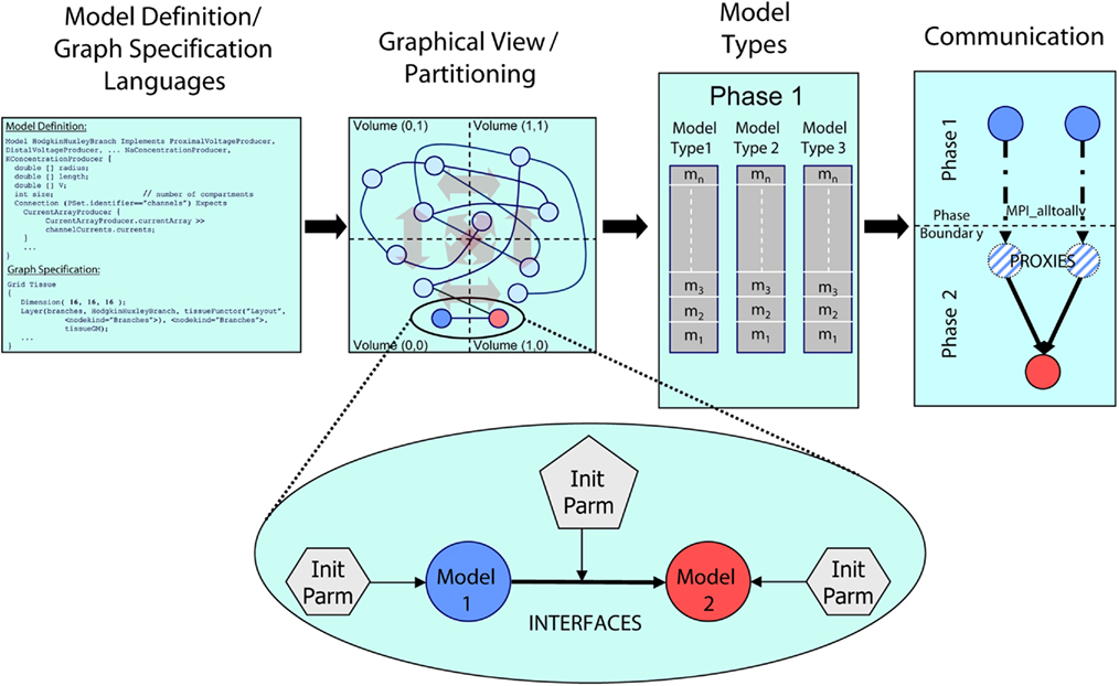
Figure 1. Architectural overview of the Model Graph Simulator. Two languages (left) define model state and interfaces (“model definition language,” MDL), and specify graph composition and connections (“graph specification language,” GSL). The specified graph is initialized and partitioned (left center). In the case of the Neural Tissue Simulator, partitioning is according to a tissue volume decomposition. Relationships between models through interfaces define connections (expanded view) and are parameterized separately from the models themselves. Models are initialized together in memory and computed by phase and by model type (right center). Communication between models (right) occurs at phase boundaries and is achieved when state from models is marshaled, communicated, then demarshaled into model proxies. Model proxies connect locally to downstream nodes to complete the connection.

Models include declared types and computational phases, executed in parallel across multiple threads referencing shared memory, multiple processes referencing distributed memory, or both. Each model is implemented once during initialization on a single computational node. It then connects to other models throughout the simulation. When a model attempts to connect to a model implemented on another node, it is noted as a sending model to that node. When a model attempts to receive a connection from a model on another node, a model proxy is created, and the connection is made from the model proxy to the model. Models sharing a computational phase have no data dependencies and reference other models or model proxies through MDL-declared model interfaces. Interprocess communication occurs only on declared phase boundaries, when data changed by models within that phase is marshaled, communicated to other processes, and demarshaled into model proxies (Figure 1).

To create the extensible Neural Tissue Simulator, we defined a core set of models in MDL (available as Supplementary Material). This list can be extended using MDL and the existing application to include any number of additional tissue components from neuroscience. The core models included:

(1) A model of a neuron branch, parameterized with the number of branch compartments, and solved implicitly at different Gaussian forward elimination and back-substitution computational phases.

(2) Two models of a junction between neuron branches (including somata), one solved explicitly at different predictor and corrector computational phases preceding and following Gaussian elimination in branches, and the other solved implicitly as part of its proximal branch.

(3) Fast sodium and delayed rectifier potassium channel models, based on the original Hodgkin–Huxley model. These channel models were coupled to all axon and soma compartments and solved in a single phase prior to all branches and junctions.

(4) Conductance-based AMPA and GABA_A synapse models (Destexhe et al., 1998) solved together with channels.

(5) A gap junction model comprising two connexons, for electrically coupling compartments from different neurons through a fixed resistance and solved together with chemical synapses and channels.

A “functor” in our simulation infrastructure is defined in MDL and expresses how the simulator instantiates, parameterizes, and connects specific models based on arguments passed to it in GSL. All functors are therefore executed during simulation initialization and iterate over specified sets of models. We designed a Neural Tissue Functor as a key component of the Neural Tissue Simulator (MDL definition available as Supplementary Material). Its arguments include a file containing a neural tissue structural specification and parameter files targeting channels and synapses to specific components of the tissue (examples available as Supplementary Material). The structural specification comprises neuron identifiers (structural layer, structural type, and physiological type) and coordinates that embed the neuron in the three-dimensional coordinate system of the tissue.

We derived the current tissue specification from cortical tissue. Unlike cortex, which scales in two-dimensions, our tissue specification scaled in three, with the sole purpose of studying the performance of the simulator and evaluating the novel numerical methods reported here for accuracy and stability. The specification included the following structural patterns:

(1) Minicolumns, comprising 20 reconstructed neurons from http://NeuroMorpho.org (Table 1; Ascoli et al., 2007) uploaded by the Markram lab (Wang et al., 2002). Each neuron was spaced at 25 μm intervals along the radial cortical axis in an order that reflects its relative laminar position in cortex, rotated randomly about the radial axis in order to ensure each minicolumn in the simulation was unique.

(2) Columns, comprising 20 × 20 minicolumns, spaced at 25 μm intervals within the two-dimensions of the cortical sheet, whose component neurons’ axons and dendrites extended hundreds of micrometers beyond the boundaries of the minicolumn or column.

(3) Tissue blocks, comprising m × n × p columns. The number of columns simulated was varied in all three-dimensions to test scaling properties of the simulator.

TABLE 1

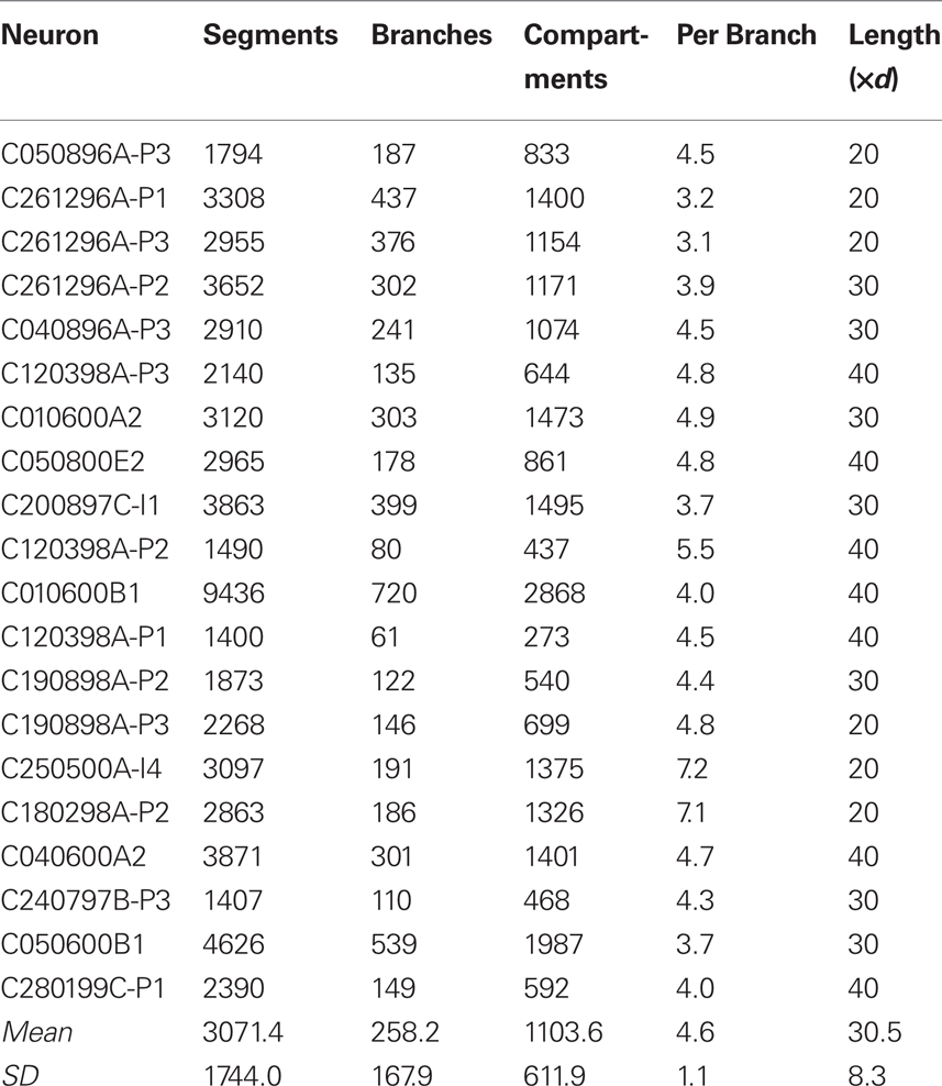
Table 1. Tissue simulation neurons.

Finally, the simulation graphs we declared using GSL (example available as Supplementary Material) express the tissue as a set of contiguous, regularly shaped volumes, each mapped to a coordinate in a three-dimensional grid. This mapping provides a means to automatically decompose the tissue into network partitions that are easily mapped onto the computational nodes and communication network topology of a supercomputer such as Blue Gene (e.g., one volume per grid coordinate per Blue Gene node). In addition, these volumes allow access to tissue components by grid coordinates. For example, recording and stimulation electrode models declared directly in GSL (i.e., not initialized by the Neural Tissue Functor) are connected to tissue components by targeting volumes according to their grid coordinates, much as real electrodes are targeted to coordinates in a real neural tissue using a stereotax.

Touch detection

The model initialization methods we employ build on existing computational techniques. First, we utilize a touch detection technique developed in our lab in collaboration with the Blue Brain Project (Kozloski et al., 2008) to generate chemical and electrical synapses during the initialization of tissue simulations. Touch detection in the Neural Tissue Simulator is performed by the Neural Tissue Functor, and involves the calculation of geometric distances between branch segments of morphologically accurate neurons in the tissue specification, where each segment in a branch is logically related to a compartment in the physiological model. By finding segments that touch, compartment pairs available for synapse creation are identified. We designed an algorithm to accomplish this task for large tissues using a parallel code that runs on the Blue Gene supercomputer. The algorithm and software architecture have been reported previously (Kozloski et al., 2008), but are reviewed here in the context of those problems and solutions they share with neural tissue simulation.

Touch detection requires performing a costly calculation of distance between two line segments up to n² times, where n is the number of branch segments in the tissue. At this upper limit, the calculation cannot possibly scale to large tissues. Fortunately, in practice, it operates on data that can be partitioned logically into local volumes within the coordinate system of the neural tissue, and then distributed to the nodes of a parallel machine. Relevant to the methods reported here, this coordinate system is identical to the coordinate system in which neural tissue simulation is performed.

Tissue volumes are right rectangular prisms created by slicing a neural tissue multiple times in each of its three-dimensions. The number of volumes created in this way equals the number of computational nodes of the machine. Slicing planes are chosen to accomplish histogram equalization of branch segments across slices in each of the three-dimensions of slicing (Kozloski et al., 2008). In this way, we approximate an optimally balanced distribution of touch detection work among the computational nodes of Blue Gene.

During work partitioning, each node of Blue Gene loads some number of unique neuron reconstructions from the structural specification, then all nodes in parallel calculate which volumes in the tissue are intersected by each of the neurons’ branch segments. Because each machine node is assigned a single tissue volume to aggregate segments for touch detection, partitioning determines which nodes receive each branch segment during redistribution of the tissue data. Whenever a segment traverses a slice plane, all nodes assigned the volumes it intersects aggregate it for touch detection. This ensures that every touch will be detected at least once. We call this method of distributing data according to neural tissue volumes a “tissue volume decomposition.”

The touch detection algorithm proceeds within each volume and on each node in parallel, creating a unique set of touches across the distributed memory of the machine, then writes touch data to disk or redistributes it for use by the Neural Tissue Functor to initialize synapses. The parallel algorithm can detect billions of touches per hour (for our largest calculation, 25.5 billion touches in 2.5 h on 4,096 nodes of Blue Gene/P (Sosa, 2008), using a new algorithm optimized to run multithreaded on Blue Gene/P’s multi-core compute nodes), emphasizing the efficiency of the tissue volume decomposition for large parallel calculations of neural tissue simulations.

Geometric constraints on touch detection may be relaxed by increasing the minimum distance between branch segments required for a touch to occur. Typically this criterion distance is defined as the sum of the two segments’ radii, but our application allows it to be increased arbitrarily. Increasing the touch criterion distance allows for the identification of more compartment pairs for possible selection and synapse creation, and thus the possibility of constructing a greater diversity of neural circuits from a single tissue by sampling a larger distribution of touches. For certain distances and certain branch types, the approach is also a reasonable model of the constraints on neural circuit development within a tissue, since dendritic spines have been identified as a critical mechanism for neurons to increase the distance over which synapses may form (Chklovskii, 2004).

An additional approach to modifying touch distributions and thus synapse creation and potential circuit configuration involves the simulation of neural tissue development. In real neural tissue, concentration and electrical gradients, and fields generated by surrounding neurons are capable of deforming the trajectory of a growing branch in predictable and stereotyped ways. They accomplish this by their interaction with sensing and motility components packed into the specialized tip of a growing branch, known as the growth cone (Hong and Nishiyama, 2010).

We created a modeling abstraction of these mechanisms and implemented a neural tissue growth simulator (Kozloski, 2011), which like our touch detection algorithm, is implemented by the Neural Tissue Functor. Here, branch segments are added to a structural model sequentially, and each is subjected to “forces” that act upon segment tips. These forces model the interactions between growing fibers and neurons, first preventing fibers from penetrating each other, and second modeling the concentration gradients of signaling molecules and local field potentials within a tissue that influence growing fibers. The simulator employs a tissue volume decomposition to distribute the work of calculating and aggregating all forces acting on a particular branch segment from other segments. In this way, neuron morphologies may be modified to achieve touch distributions different from what is possible by incorporating rigid neuron morphologies into a simulated tissue and increasing the touch distance criteria. Finally, because each branch segment type can be parameterized to generate and sense a unique and arbitrary set of forces within the tissue, the dynamics of neuronal growth, and the mapping from a set of developmental parameters to stereotyped microcircuit structure and function may be studied. Our parallel, multithreaded algorithm has successfully simulated the growth of axons for a single column (8,000 neurons) on 4,096 nodes of Blue Gene/P in 24 h (Kozloski, 2011).

Volumetric data decomposition, local synapses, and exploiting link bandwidth

The neurons in the neural tissue simulations we used to test the Neural Tissue Simulator (Table 1) are reconstructions of real neurons, rotated and positioned within simulated tissue blocks and connected via synapses and gap junctions to neighboring neurons. Neurons consisted of a soma, an axon, and one or more dendrites, with O(100) branches and O(10,000) chemical synapses per neuron, as well as a very small number of gap junctions per neuron (<10), which couple dendrites of inhibitory interneurons, and axons of excitatory pyramidal and spiny stellate neurons. Axons and dendrites are composed using the same branch models, and are indistinguishable in their numerical solutions, despite different couplings to channel models (i.e., different channel types and densities)². Neurons are decomposed into branches, branch points, and somata, which in turn are decomposed into compartments. Branches comprise one or more compartments, while branch points and somata correspond to a single compartment each. All of a neuron’s coordinates are relative to the (x, y, z) center of the soma, and undergo rotation and translation about this point before insertion into the tissue coordinate system. Coordinates and radii are then resampled to create a neuron comprising a contiguous set of tangent spheres, each bounded by the hull of the original reconstruction. In this procedure, branch points may be displaced slightly when the last tangent sphere in a branch is created. Spheres are downsampled by reserving the first sphere of some regular sphere interval (for example, “1 every 10”) and the last sphere of a branch. The reserved spheres then demarcate the endpoints of compartments. The result of this process is the creation of O(1,000) branch compartments per neuron, each of which is described by two endpoints (i.e., sphere centers) and a radius. The somata and branch point compartments are then described by single spheres within this scheme.

Unlike previous approaches, neurons are divided at points within branches where a single branch intersects a slicing plane and is divided into two branches (i.e., at “cut points”). A single neuron is therefore most often mapped to multiple machine nodes in our data decomposition. The neural tissue is first divided into volumes by the Neural Tissue Functor and each volume assigned to a machine node. Slicing planes are chosen to accomplish a weighted histogram equalization of compartments across slices in each of the three-dimensions of slicing. Weights for each compartment are calculated based on a sum of weights of its associated channel and branch models. These weights were determined experimentally and reflect the expected computational load of each model. In this way, we approximate an optimally balanced distribution of work for solving branches on the computational nodes of Blue Gene. Each compartment is then assigned to the volume containing the compartment’s proximal endpoint (except for branch points, which are assigned to the same volume as their proximal compartment) and initialized on the machine node assigned their volume (Figure 2). Initialization of branches proceeds as compositions of consecutive branch compartments and junctions are assigned to the same volume. As a result, branches whose compartments were assigned to more than one volume are effectively cut into multiple branches (Figure 2). The Neural Tissue Functor is responsible for initializing branches and junctions, and their proxies, in order to ensure that the Model Graph Simulator’s collective communication is consistent and matched across all volume boundaries (node–node pairs; Figure 2).

FIGURE 2

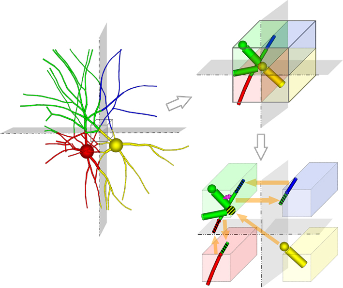
Figure 2. Tissue volume decomposition and creation of models and model proxies depicted as two neurons embedded in a tissue, and sliced along two orthogonal planes. The Neural Tissue Simulator slices along three planes. Computation of the neuron is decomposed into models (branches and junctions) which are initialized in different volumes (represented by their different colors). Synapses are also initialized within the volumes containing their presynaptic and postsynaptic compartments (magenta). A portion of these volumes is expanded (cube; upper right) to depict models that span the slicing plane. To support communication between these models (lower right) model proxies are initialized (striped colors) such that models that connect to models in other volumes do so via a model proxy on that volume. Communication occurs once between computational nodes on each phase boundary, requiring state from models to be marshaled and demarshaled into proxies.

For a parallel architecture, link bandwidth typically measures the number of bytes per second that can be communicated from one machine node to another through any number of wires that connect the pair directly. Despite some overhead involved in sending data in packets, link bandwidth is a good estimate of the effective bandwidth between adjacent nodes on the machine’s communication network (Al-Fares et al., 2008).

Because not all nodes are adjacent on today’s large parallel machines, a network topology determines the number of links that separate nodes. For Blue Gene/P, this topology is a three-dimensional torus, which attempts to maximize the bisection bandwidth of the machine, while ensuring that a large number of adjacent nodes (nearest neighbors) exist for any node on the network. Bisection bandwidth is the bandwidth across the minimum number of links that divide the machine into two partitions with equal numbers of nodes (Al-Fares et al., 2008) and determines the amount of time required for all nodes to communicate to all nodes, (typically referred to as “all to all” communication). For Blue Gene/P, link bandwidth is maximum between nearest neighbors and measures 6.8 GB/s, while bisection bandwidth varies between 1.7 and 3.8 TB/s, depending on the machine size (Sosa, 2008).

The Neural Tissue Simulator exploits nearest neighbor communication in the massively parallel architecture of Blue Gene to create fixed communication costs that are wholly dependent on the local structure of neural tissue (Figure 3). Because synapses, like neuron compartments, are simulated as structural elements embedded within the tissue’s three-dimensional coordinate system, the communication cost for most synapses is zero, since nearly all components of each synapse are wholly contained within a single tissue volume (Figure 2). State necessary for modeling synaptic transmission as a coupling between presynaptic voltages and postsynaptic conductance changes (Destexhe et al., 1994) is therefore referenced within local memory of a single machine node rather than requiring a costly communication over the machine’s network.

FIGURE 3

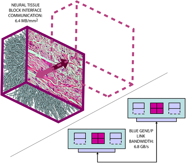
Figure 3. The Neural Tissue Simulator exploits a tissue volume decomposition, and therefore communication in a simulation of arbitrary scale can be estimated. This is due to all communication occurring at interfaces between neural tissue blocks, where a micrograph (courtesy of the Department of Histology, Jagiellonian University Medical College and Wikipedia.org) can provide sufficient information to perform the estimate. Here we estimate based on our models from the Neural Tissue Simulator a communication requirement which can be accommodated easily by the link bandwidth between Blue Gene/P’s node cards.

Because communication across synapses by simulation elements imparts almost no additional machine network communication cost, the marginal cost of adding a synapse to a simulation is therefore the constant cost of computing the synapse’s state and current (Figure 4). In our study of simulations comprising 256,000 neurons on 1,024 nodes of Blue Gene/P, while varying synapse counts from 0 to 11,265 per neuron, the measured cost was approximately 50 μs per synapse per simulated second³. This negligible linear relationship between number of synapses and compute time has profoundly favorable implications for simulations that aim to replicate the physiological and anatomical constraints imposed by real neural tissue (Markram, 2006), where synapse densities may approach one per cubic micron (Braitenberg and Schuz, 1998), and synaptic counts per postsynaptic neuron easily achieve 10⁵–10⁶ (for example in neocortex and cerebellum).

FIGURE 4

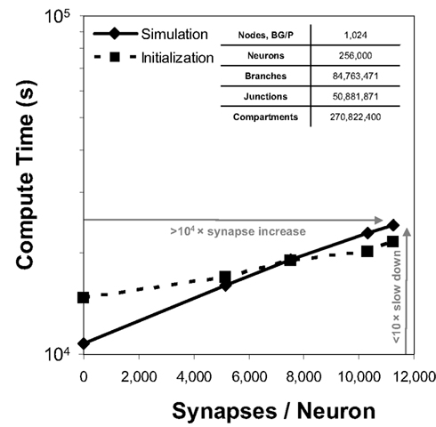
Figure 4. Synapse scaling. Plot of both initialization times and simulation times (100 ms of physiology) vs. synapses/neuron for a constant number of neurons on a fixed machine size (inset table). Increasing synapse density by four orders of magnitude causes compute time to approximately double.

Thus, in our tissue volume decomposition, nearly all communication in a simulation occurs between adjacent nodes of Blue Gene/P and traverses only one link. Communication efficiency in our simulation is therefore determined by link bandwidth not bisection bandwidth. For this reason, the amount of data communicated over links remains constant as the size of the simulation grows proportionally with the size of the machine (i.e., its number of nodes). In contrast, poor scaling almost always results from network congestion due to irregular communication patterns that require longer communication paths and/or greater message lengths as the simulation and machine size grow, though at the scale of present neural tissue simulations, this does not appear to be the case for other approaches (Hines et al., 2008b; Kumar et al., 2010).

Our tissue volume decomposition is able to exploit Blue Gene’s innovative toroidal network topology because it provides a natural mapping from nearest neighbor volume to volume communication in a neural tissue to nearest neighbor node to node communication on the machine’s network (Figure 3). Thus, while other applications employ a neuron decomposition, equating communication between nodes with the communication between neurons in a network, our volume decomposition employs node to node communication that models the fixed planar interfaces between neural tissue volumes. We exploit the fact that these fixed planar interfaces have a fixed cross-sectional composition determined by the ultrastructure of neural tissue, resulting in a fixed communication cost per unit area.

Despite the constraints and advantages of nearest neighbor communication, the communication engine we devised for the Neural Tissue Simulator supports communication across all possible paths in the network and uses only the MPI_Alltoallv communication collective. We chose this collective for communication at iteration phase boundaries (Figure 1) for two reasons. First, under certain rare circumstances, compartments, or synapses may span non-adjacent nodes (for example if a compartment is very long), and therefore the calculation of a branch or synapse’s state within a time step will require communication through multiple links on the network. More significantly, we aimed to support models that require global communication (for example, models of EEG, deep brain stimulation, etc.). We do not report results for simulations using these globally communicating models since we aimed here to study only the scalability of fundamental simulation functions of the Neural Tissue Simulator. We anticipate that the scaling properties reported here will be minimally impacted when such models are added however, due to the high bisection bandwidth of the Blue Gene architecture, and its optimized collective communication (Almasi et al., 2005).

Scalability

Initialization of the simulation has three stages: tissue development, touch detection, and physiological initialization (each performed by the Neural Tissue Functor). We showed previously that both tissue development and touch detection scale with the number of branch segment interactions (i.e., touches, forces, etc.) calculated within a volume (Kozloski et al., 2008; Kozloski, 2011). Our tissue volume decomposition therefore allows for both strong scaling, where the total number of interactions is held constant and the number of volumes increases (resulting in a constant decrease in compute time) and weak scaling, where the number of interactions and the number of volumes grows proportionally (resulting in a constant compute time). For larger touch criterion distances or longer range forces, however, these scaling properties break down as interactions must be computed in more than one volume, and the algorithms lose the benefits of parallelism. Fortunately, the need for either long distance touch criteria or long range force calculations is typically small in neural tissue simulations, and their number much less than the total number of branch segments [for example, typically only axons are subjected to long range forces, while all branches experience short range forces due to direct physical interactions (Kozloski, 2011)].

Physiological initialization requires iterating through branch segments and touches, and identifying which segments require connections to local instantiations of the neural tissue models, and which must connect to model proxies (Figures 1,2). Making this distinction involves multiple searches of multiple maps that relate the various models to each other, and to the tissue volume decomposition. These searches, using Standard Template Library map containers, proceed with O(logN) complexity, such that if the amount of tissue (N) that must be searched within a volume grows, initialization may be slowed. We note the importance then of limiting the size of tissue volumes in order to ensure timely initialization, which is readily achieved using massively parallel machines such as Blue Gene. During the study reported here, we continued to optimize physiological initialization, for example by improving our disk access times for reading the tissue structural specification. Our results indicate that both strong and weak scaling are properties of all three stages of initialization performed by the Neural Tissue Functor, with expected total initialization times of 1–2 min per neuron per processor across all simulation and machine sizes reported here with on average 10,000 synapses per neuron. Furthermore, the relationship between synapses per neuron and initialization time is linear over the physiological ranges we studied (Figure 4).

Numerics

Our model simulation methods build on existing numerical approaches for solving Hodgkin–Huxley type mathematical models of branched neurons, as described in Supplementary Information. Here we report our numerical approach to solving these equations, which can be considered a tunable hybrid of Hines’ method (Hines, 1984), and that of (Rempe and Chopp, 2006). We first review the two methods, emphasizing aspects relevant to our hybrid. We then discuss how our approach allows for novel adjustments to the decomposition of a neuron into implicitly solved tree partitions separated by explicit junctions, and how using our tuning parameter (“maximum compute order”), a trade off occurs between the numerical stability and accuracy of the combined method, and the efficient parallel execution of the computational algorithm that implements it.

The Hines algorithm

The “Gold Standard” for numerically solving Hodgkin–Huxley neuron models is the Hines algorithm (Hines, 1984), which improved and extended to branched neurons the numerical scheme originally proposed by Cooley and Dodge (1966) for computing action potentials in a cable. Cooley and Dodge showed that a backward implicit scheme for computing the membrane potential, combined with an iterative scheme for solving the non-linear channel equations, could be used to efficiently implement the second-order accurate Crank–Nicholson method for Hodgkin–Huxley type models. Hines provided two critical insights. First, he showed it is possible to maintain second-order accuracy while eliminating the need to iterate when solving the channel state equations by staggering the time points at which the membrane potential equations and channel state equations are satisfied. He then derived a branch and compartment numbering scheme that made it possible to construct a single linear system for a branched neuron that can be diagonalized efficiently. This numbering scheme corresponds to a depth-first visit of branches and compartments, where the soma is considered the root of multiple trees corresponding to axons and dendrites.

These observations, combined with a fully implicit, nearest neighbor numerical method (Figure 5A), produced a linear system that is tridiagonal except for rows and columns corresponding to branch points, yet can still be diagonalized efficiently using a slight modification to the Thomas algorithm (Thomas, 1949; Bruce et al., 1953). Such a scheme makes it impossible to solve arbitrary branches of a single neuron simultaneously using a parallel machine, though subtrees that originate at the same neuron root have been successfully solved in parallel (Figure 5B; Hines et al., 2008a), and neuron splitting techniques have now been extended to take many forms (Hines et al., 2008b). Furthermore, this fully implicit approach yields a stable and accurate solution at the level of the neuron, even when neurons are coupled via chemical synapses, but can not be extended to include electrical synapses (Hines, 1984). As a result, when applied to a tissue containing electrical synapses, Hines’ approach must be modified to include explicit terms everywhere electrical synapses occur. This has the effect of decoupling the neurons, which can then be solved implicitly. The introduction of explicit terms and fixed-point iteration to solve for electrical synapses limits the stability and accuracy of the overall numerical method, however. Moreover, these explicit terms occur wherever electrical synapses occur, rather than at specific, well-defined locations like junctions, such that their numerical effects may be difficult to control.

FIGURE 5

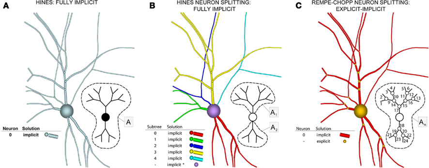
Figure 5. Components of our numerical approach. (A) The Hines algorithm (left) solves the entire neuron implicitly (indicated by blue), represented here as a neuronal arbor comprising branches, compartments, and implicit junctions. Inset image depicts how a parallel solver can calculate this solution, with the matrix A representing the portion of the neuronal arbor that must be solved in a single phase (i.e., the whole tree). (B) Hines’ neuronal splitting algorithm allows different trees originating from the soma to be solved separately and implicitly, here depicted by different colors. The soma is then solved in a manner Hines describe as implicit equivalent (purple). Inset depicts each tree solved in parallel, assigning a different subscript to matrices A_n to represent this parallelism (dotted lines demarcate different trees). (C) Rempe–Chopp’s explicit algorithm transforms each branch point into an explicit junction (orange) and all branches can be solved implicitly and in parallel (inset; wherein the matrix A_n indicates parallelism, its subscripts labeled on each branch, and the dotted line demarcates all instances of A_n).

The Rempe–Chopp algorithm

In contrast to Hines’ approach to solving the neuron’s membrane potential with an implicit numerical scheme and a single linear system for the entire neuron, Rempe and Chopp (2006) decomposed the neuron into implicitly solved branches, and introduced an explicit predictor–corrector scheme for the membrane potential at branch points (Figure 5C). In this approach, an explicit step is used to predict the value of the membrane potential at the branch point at the forward time. This predicted value is then used in place of the junction’s unknown membrane potential in solving for the membrane potential at the forward time in the branches to which the junction is attached. Once the membrane potential at the forward time in the branches is determined, the value is used to correct the membrane potential at the branch point at the forward time. This approach effectively decouples the solution of the membrane potential between branches, permitting an implicit scheme within each branch. Hines’ large linear system is thus replaced with a set of much smaller linear systems that are truly tridiagonal and decoupled from each other, and can therefore be solved efficiently and simultaneously in parallel within a single neuron. Their approach also lends itself to computational gains derived from spatially adapting solutions depending on gradients in the membrane potential within each branch, a technique that is greatly aided by the decomposition and the simple computation of individual branches (Rempe and Chopp, 2006; Rempe et al., 2008).

It is important to note that Rempe and Chopp (2006) formulated the problem in the same fully implicit manner as Hines, but utilized an explicit, predictor–corrector approach to estimate the solution at all junctions. As Hines noted, “Very strong coupling between adjacent compartment voltages demands implicit methods for numerical stability with reasonable time steps” (Hines, 2008a), and so Rempe and Chopp’s (2006) approach limits the stability and accuracy of their numerical method at junctions, and therefore of the method overall. Surprisingly however, they were able to show empirically that their method was sufficiently stable and accurate to permit use of a reasonable time step. They found time steps up to O(100) μs produced stable and accurate solutions for the classic Hodgkin–Huxley model on branched structures comprising branches 80 μm long with radii of 0.2 μm and compartment spacings of 8 μm. Moreover, on complex, branched structures, their method matched that of Hines at a time step of 15 μs.

The sizable approximations made in constructing these models, combined with the stability properties of Rempe and Chopp’s method, permit a reasonable choice between the accuracy found in Hines’ method and the speed increase that Rempe and Chopp’s method allows via parallelization and spatial adaptation. Our method implements this choice in a manner tunable by a single parameter.

A hybrid branched cable equation solver

We developed a hybrid method that trades off the accuracy and stability afforded by Hines’ fully implicit numerical method (Hines, 1984) and the parallelism made possible by Rempe and Chopp’s (2006) implicit/explicit numerical method for solving a neuron’s branched cable equations. We describe the mathematics of our hybrid method in Supplementary Information. Here we describe the computational approach and illustrate the trade off graphically. The computational method of the Model Graph Simulator requires identification and ordering of specific phases of a model’s computation so as to eliminate data dependencies between models. For Rempe and Chopp’s method, these phases are the predictor and corrector steps of the explicit junctions’ calculations, separated by a fully implicit solution phase for branches between them (Figure 5C).

Now consider a fully implicit parallel solver that replaces all explicit junctions between branches with implicit junctions (Figure 6A). In this approach, which we also implemented using the Model Graph Simulator, all branches of a particular branch order (defined neuroanatomically as the number of junctions between the branch and the soma) are computed within a single phase, and branches of different branch orders are assigned to different phases. Specifically, branch order phases are structured such that the maximum branch order’s Gaussian forward elimination phase occurs first, followed by the next highest branch order, and so on until finally zeroth order branches undergo both a forward elimination and a back-substitution phase. Each subsequent branch order then undergoes back-substitution until all branches are solved. At each implicit junction (solved with the proximal branch to which it is connected), the numerics of Hines’ approach are applied to solve the off diagonal elements of the branched cable’s matrix.

FIGURE 6

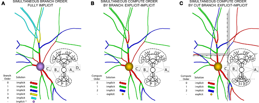
Figure 6. Creation of our numerical approach. (A) Different branch orders may be computed in parallel across the entire neuronal arbor (represented by different colors). All junction are computed implicitly. Inset shows various matrices A_n–D_n representing the portion of the neuronal arbor that must be solved in a single phase (i.e., whole branch orders). Subscripts label branches indicating all branches of an order may be solved in parallel, and dotted lines also demarcate branches of an order. (B) By introducing the concept of compute orders, we introduce explicit junctions at a fixed branch order interval (in this case, determined by a maximum compute order of 2). This allows different branch orders to be computed in parallel (e.g., 0 and 3). Colors, matrices, subscripts, and dotted lines as in (A,C) By slicing the neuron tissue, additional explicit and implicit junctions are introduced at cut points, and all distal compute orders are incremented. The numerics of distal junction may also change. Colors, matrices, subscripts, and dotted lines as in (A).

The advantage of this approach is that all branches of the same branch order can be solved fully implicitly and in parallel, allowing a tissue volume decomposition to assign branches to machine nodes based on volume, where volume boundaries introduce additional implicit or explicit junctions at cut points. The disadvantage is that the proliferation of computational phases as neurons grow in complexity (approaching the physiological range of 10–10² branch orders) requires a synchronization point in the parallel algorithm wherever communication between contiguous branches of different orders occurs, each of which imposes a cost on performance of the parallel simulation.

An alternative approach incorporates Rempe and Chopp’s explicit junctions at select points in the neuron’s branched arbor (Figure 6B). We define a compute order as the branch order modulo one plus a specified maximum compute order. By replacing branch order computational phases with a smaller number of compute order phases we address the problem of excessive synchronization points associated with a fully implicit branch order approach. Therefore, with a maximum compute order of 0, Rempe and Chopp’s approach is replicated with all junctions being explicit. With the maximum compute order equal to the highest branch order of the neuron, Hines’ approach is replicated with all junctions being implicit. We designed the Neural Tissue Simulator to allow specification of an arbitrary maximum compute order between these two values. With intermediate values, a trade off is achieved between solving a larger portion of the neuronal arbor implicitly, while maintaining a reasonable number of computational phases and synchronization points in the parallel algorithm (Figure 6B). To achieve a volume decomposition, additional junctions (either implicit or explicit) may be added at cut points between volumes, thereby altering all distal compute orders, and changing the numerical approach (explicit/implicit) for solving certain distal junctions (Figure 6C).

For a test simulation of 128,000 neurons, 42 million branches, and 135 million compartments on 512 nodes of Blue Gene/P, we varied the maximum compute order from 0 to 7 (Figure 7) and observed a reduction in the number of explicit junctions of ∼25% per additional compute order. Fewer explicit junctions increased the size of implicitly solved neuron branch partitions and so presumably improved the stability and accuracy of our simulation (instability was never observed). Surprisingly, we also observed that simulation performance decreased very little as 2–12 additional synchronization points for communication between implicit branches were added (one forward elimination and one back-substitution communication per compute order; 0.4–4% slow down per additional compute order). Furthermore, initialization compute time was impacted even less by additional compute orders.

FIGURE 7

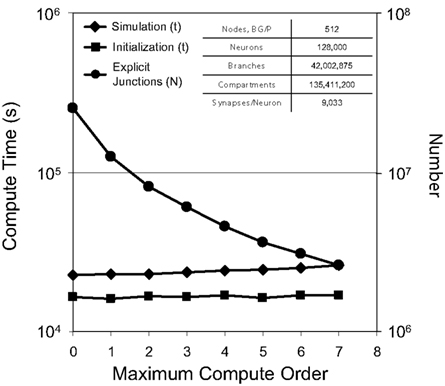
Figure 7. Compute order scaling. Plot of both initialization times and simulation times (100 ms of physiology) vs. maximum compute orders from 0 to 7 for a constant number of neurons on a fixed machine size (inset table). On the right y-axis, number of explicit junctions over the same maximum compute orders is plotted.

Our test simulations used a time step of 10 μs, which compares favorably to that used in previous work when compartment size is taken into account. The largest published simulation to date, for example, utilized a time step of 25 μs in simulating approximately 300 electrical compartments in 300 branches per neuron, and did not explicitly model the axon (King et al., 2009). Our model neurons comprised 1,104 ± 612(SD) compartments in 258 ± 168(SD) branches (Table I), or 4.6 ± 1.1(SD) compartments per branch. This resulted in compartment lengths ranging from 20 to 40 times the fiber diameter. Given that for parabolic equations, Δt ∼ Δs², it is reasonable to employ a smaller time step for the smaller compartments, since even for the unconditionally stable, fully implicit Crank–Nicolson method, accuracy is controlled by the local truncation error, which is O(Δt²) + O(Δs²). Explicitly modeling the propagating action potential in the axon also imposes additional constraints on the time step.

Simulation Workflow

Here we provide a step by step sequence for the workflow of simulation initialization and execution, complete with required data inputs, calculations, and outputs. Note that all steps following model code generation are executed by a single executable run on Blue Gene/P.

(1) The MDL parser compiles MDL (see Supplementary Material) into C++ for models and functors, generating a single code to run on multiple platforms. The MDL parser generates code stubs for implementing model and functor behavior. The simulation designer then implements model functionality in C++.

(2) A configure script initiates C++ code compilation, targeting the executable for a specific platform (Blue Gene/P for this study).

(3) The mpirun command is issued on Blue Gene/P. Because all simulation compute threads are bound to cores on Blue Gene/P, an additional set of non-bound threads for initialization and communication are created using an environmental variable. Other environmental variables specify the maximum message size and the machine mode on Blue Gene/P. Arguments passed to the GSLparser executable (which parses GSL and creates and runs the simulation) configure the number of threads and the GSL file name. For example:

mpirun -env “BG_APPTHREADDEPTH=2 DCMF_RECFIFO=48000000”
-partition r0 -c4096 -np 4096 -mode SMP -cwd /NTS
-exe /NTS/bin/GSLparser -args “-t 4 Tissue0.gsl“

(4) The GSL parser reads GSL (see Supplementary Material) and initializes the tissue volume grid based on GSL specified grid dimensions. The grid specifies a set of grid layers, each of which comprises a single model type that the Tissue Functor will generate. Note that “layer” does not refer to a structural layer, but to a set of functional model “overlays” within each grid coordinate (volume) in the tissue. In this way, different types of channels, synapses, and compartments can be generated and accessed within the grid.

(5) A volume mapper assigns each volume to a node of Blue Gene/P, ensuring that tissue volume and node coordinates preserve nearest neighbor communication patterns on the hardware.

(6) The Tissue Functor reads the tissue specification file and computes a globally consistent scheme for dividing neuron-related initialization work. The functor loads different neurons from .swc files into memory according to this scheme onto each node of the machine.

(7) The Tissue Functor performs a resampling algorithm, transforming neurons in memory by creating points spaced at regular multiples of their containing fibers’ diameters.

(8) Communication between all nodes of the machine enumerates all points in the tissue, constructing a global point histogram, which is then equalized in three-dimensions to create a volume slicing.

(9) Neuron segments are communicated to all volumes they traverse, according to the volume slicing scheme.

(10) The Tissue Functor executes a neuron growth algorithm (optional), sequentially adding each segment of each neuron while subjecting each segment to specified forces from segments already in the tissue.

(11) The Tissue Functor executes a touch detection algorithm, and computes touches between all neuron segments in each volume. Touches are detected using a parameterized probability, which may save memory in extremely dense tissues. Globally consistent random number generation allows touch detection to remain consistent across all nodes of Blue Gene/P.

(12) The Tissue Functor aggregates computational costs associated with each neuron segment based on cost estimates for compartments, channels, and synapses, provided by a simulation designer in a .par file (see Supplementary Material). A global histogram of costs is then equalized in three-dimensions to create a second volume slicing scheme for work distribution, which ensures the computational load is balanced.

(13) With this scheme, the Tissue Functor communicates touches and neuron segments to nodes of Blue Gene/P responsible for implementing models or model proxies that depend on these data (for example synapses, each of which depends on one touch and two segments, and compartments, each of which depends on a segment). A simulation designer provides parameterized mappings in .par files (see Supplementary Material) that constrain which models are created based on a specified association between GSL model indices and branch identifiers associated with each neuron segment and touch in the tissue specification.

(14) The GSL parser creates all tissue models, including branches, channels, and synapses. A simulation designer parameterizes in a .par file (see Supplementary Material) the probability of creating synapse models of a specific type from a set of valid touches.

(15) The GSL parser initializes other models such as stimulation and recording electrodes, connecting each to specified models within the tissue. In addition, specified simulation triggers (for example, to control data collection and simulation termination) are initialized.

(16) The GSL parser interprets the specified phase structure of the simulation and maps different models’ phases to declared simulation phases.

(17) The GSL parser initiates the simulation, in which each iteration comprises a sequence of phases that: solve ion channel and synapse states, predict branch junction states, forward eliminate branches of appropriate compute orders, back-substitute branches of appropriate compute orders, correct branch junction states, evaluate all triggers, and collect data if necessary. Between each phase, model state modified during a phase and required by other models is marshaled, communicated by MPI_Alltoallv, and demarshaled into model proxies.

(18) The simulation terminates when the end criterion is satisfied. All models and simulation data are destructed on all nodes of Blue Gene/P.

Public Availability of Data, Simulation Specifications, and Simulator

All neuromorphological data presented derive from the publicly accessible database found at www.neuromorpho.org. Scripts written in MDL and GSL, and an example tissue specification and parameterization files for creating and running the largest simulation reported here, are available as Supplementary Information. The Neural Tissue Simulator software is experimental. IBM would like to create an active user community. Readers are therefore encouraged to contact the authors if interested in using the tool or in the source code.

Simulation Scaling Results

Here we report the results of scaling the Neural Tissue Simulator using several methods in order to evaluate its performance over a variety of simulation and machine sizes and configurations.

Thread Scaling

The Blue Gene/P runtime system allows applications to run in symmetric multiprocessor “(SMP) Mode,” wherein each of its 4 core nodes is equivalent to a SMP machine (Sosa, 2008). In this mode, computational threads may be created by the program and run simultaneously on the node’s different cores, each referencing the same shared node memory. Our Model Graph Simulator fully exploits SMP machines, parallel distributed memory machines such as clusters, and hybrid machines such as Blue Gene/P (Kozloski et al., 2009). In simulations used to test the Neural Tissue Simulator, the four threads of each node compute models within a phase simultaneously in SMP mode. Models then reference the state of other models on the same node (even if computed by other threads) directly at their location in memory, rather than through MPI communication and model proxies, which are reserved strictly for node to node communication. Such a capability can be valuable, especially since subsequent generations of Blue Gene will have significantly more cores each supporting an additional thread.

We observed thread scaling in our test simulations of 128,000 neurons, 40 million branches, and 135 million compartments on 512 nodes of Blue Gene/P (Figure 8). Different simulation runs specified different numbers of threads (and thus utilized different numbers of machine node cores). The speed up observed from 1 thread to 2 was 1.8×, from 2 threads to 3 was 1.4×, and from 3 threads to 4 was 1.3×. Overall, we observed a 3.1× speed up from 1 thread to 4. We anticipate therefore that the Neural Tissue Simulator will effectively exploit additional threads on architectures with more cores per node, as this scaling appeared sufficiently near optimal to continue beyond Blue Gene/P’s core constraints.

FIGURE 8

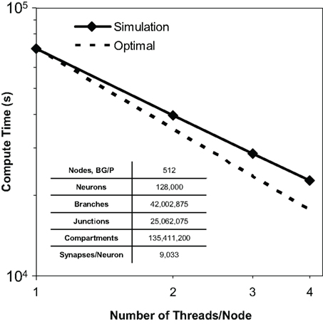
Figure 8. Thread scaling. Plot of simulation times (100 ms of physiology) vs. number of threads used in SMP mode on Blue Gene/P per node for a constant number of neurons on a fixed machine size (inset table). Optimal thread scaling (dotted line) is shown for comparison.

Strong Scaling

Strong scaling refers to the ability of an application to perform the same sized calculation faster on machines of larger sizes. We observed strong scaling of the Neural Tissue Simulator when we performed a simulation of 16,000 neurons on Blue Gene/P machine sizes ranging from 64 to 4,096 nodes (Figure 9). Simulations continued to speed up even as more branches were divided into separate models by our tissue volume decomposition, potentially impacting scaling negatively.

FIGURE 9

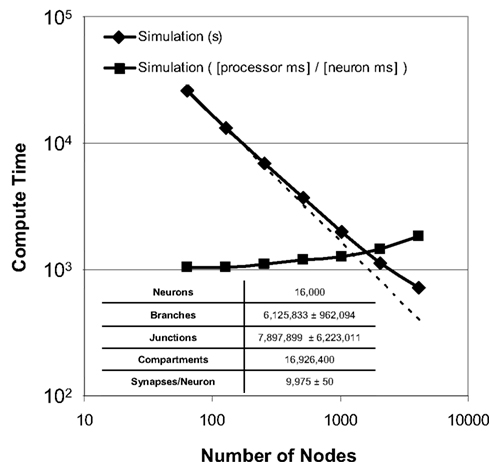
Figure 9. Strong scaling. Plot of simulation times (100 ms of physiology) vs. number of computational nodes (4 cores/node) on Blue Gene/P for a constant number of neurons (inset table). Optimal strong scaling (dotted line) is shown for comparison. Scaling numbers are normalized and plotted a second time, and both plots show strong scaling to 4,096 nodes (16,384 cores) of Blue Gene/P.

To express performance results in units more relevant to neural tissue simulation, we normalized the simulation times and expressed them in terms of the amount of time each processor of any machine must compute in order for the entire machine to compute a given amount of physiological time for a single neuron. We measured this time at 1.0 processor seconds per neuron millisecond when there is an average of 250 neurons per node, and 1.8 for an average of 4 neurons per node. Thus, while strong scaling could likely continue to produce shorter overall simulation times on machines larger than those we used, the normalized measurements indicate that the benefit of larger machines for problems of this size will likely diminish.

Weak Scaling

Weak scaling refers to the ability of an application to perform calculations of varying sizes in the same amount of time, provided that as the calculation size grows, the machine size grows proportionally. We observed excellent weak scaling of the Neural Tissue Simulator when we performed simulations of different sizes while holding the average number of neurons per node constant at 250 on Blue Gene/P machine sizes ranging from 64 to 4,096 nodes (Figure 10). Simulation times decreased by 15% from 64 nodes to 4,096 as the simulation size increased from 16,000 to 1,024,000 neurons. The normalized simulation times decreased from 1.0 processor seconds per neuron millisecond to 0.88. Thus the largest simulation we performed during this weak scaling study calculated 100 ms of neurophysiology for over 1 million neurons, 1 billion compartments, and 10 billion synapses (Table 2) in 6.1 h.

FIGURE 10

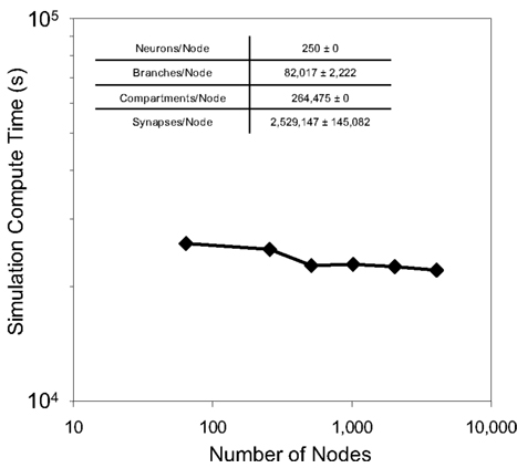
Figure 10. Weak scaling. Plot of simulation times (100 ms of physiology) vs. number of computational nodes (4 cores/node) on Blue Gene/P for a constant average number of neurons/node (inset table). This plot shows weak scaling to 4,096 nodes (16,384 cores) of Blue Gene/P.

TABLE 2

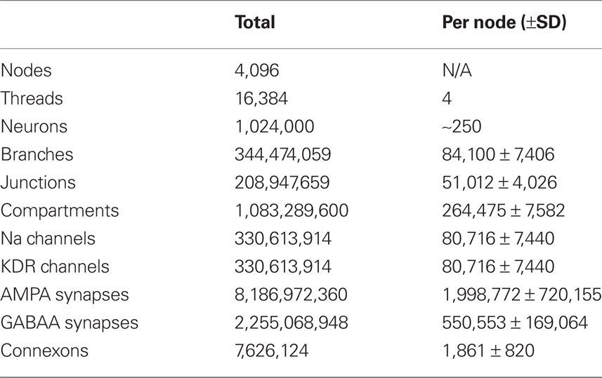
Table 2. Scale of largest simulation: neural tissue simulator.

Discussion

Implications of Results

The simulations we performed, while intended to test the performance and scaling of a parallel application for calculating the Hodgkin–Huxley equations for branched neurons using a novel tissue volume decomposition, has provided additional physiological results worth noting. Specifically, we observed by recording simultaneously from many basket cell interneurons in the upper layers of our tissue simulations, action potentials that originated in the axons then back propagated into somata, where they failed to regenerate full scale action potentials (Figure 11). This observation emphasizes the importance of simulating the compartments of axons, in part because sodium channel densities were constant throughout the axonal arbor. Furthermore, complex synaptic integration of the massive AMPA and GABA_A input to each neuron is evident in the dendritic voltage traces. These observations provide confirmation that our simulations and their novel numerical methods are capable of replicating normal physiology similar to that observed from the same neurons in vivo (Wang et al., 2002). They further demonstrate the value of the approach of specifying neural tissue simulations from structural files comprising real neuron reconstructions and synapses placed by touch detection (Markram, 2006; Kozloski et al., 2008).

FIGURE 11

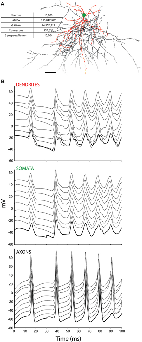
Figure 11. Physiology of basket cells. (A) Recordings were made from nine instances of a single basket cell morphology in a simulated tissue (scale bar is 100 μm; inset table). (B) Recordings were made from a point in the dendrites, somata, and axons of each neuron. Here we plot the first only at the correct scale of the recorded voltage. Each subsequent trace is offset by 10 mV to allow inspection and comparison. A current of 500 pA was injected into the first somata at time 30 ms, and remained on for the duration of the simulation.

Furthermore, while previous neural tissue simulations employ fewer synaptic inputs than we show here, the Neural Tissue Simulator clearly achieved physiological scales of synaptic inputs (∼10,000 synapses/neuron), in part due to our tissue volume decomposition’s local calculation of synapses. Furthermore, we note that an average additional 510 synapses/neuron had a significant effect on recordings from the same neurons’ somata (Figure 12), even when all other simulation parameters were held constant.

FIGURE 12

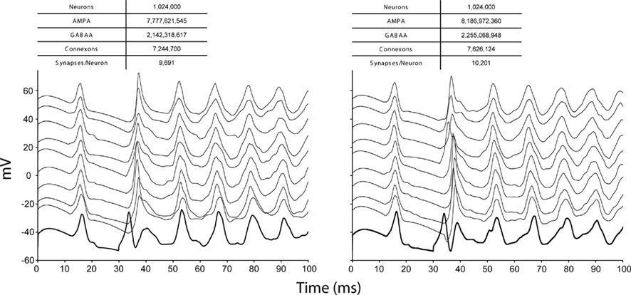
Figure 12. Physiology of a very large tissue at different synapse densities. Recordings from 10 instances of the same basket cell morphology as in Figure 11 in a very large simulated tissue (inset table). Recordings were made from the somata. Again, we plot the first only at the correct scale of the recorded voltage, and each subsequent trace offset by 10 mV to allow inspection and comparison. A current of 500 pA was injected into the first somata at time 30 ms, and remained on for the duration of the simulation. Synapse densities were increased by 510 average synapses/neuron from the left to right panels.

Finally, these recordings represent the first from a tissue simulated at this scale (>1 million neurons, comprising on average 1,104 compartments/neuron; Table 2). We anticipate that because of the excellent weak scaling demonstrated here (Figure 10) as machine sizes grow in the future, the simulation sizes achievable by the Neural Tissue Simulator and its tissue volume decomposition will continue to grow proportionally, while simulation times will remain constant. This ultrascalable solution therefore has profound implications for the future of neural tissue simulations, and suggests that human brain scale neural tissue simulations are not only feasible but likely within the next decade. We will now discuss in greater depth the feasibility of human brain scale simulations based on our scaling results from the Neural Tissue Simulation.

Feasibility of Human Brain Simulation

Estimating the computational requirements for simulating an entire human brain is difficult for a number of reasons. First, though neural tissue simulation is technically most suited to making this estimate (for reasons we list below), neuroscience still has no predictive models for global brain function. Without consensus on which modeling approach is most functionally appropriate for whole-brain simulations, any estimate will require an assumption-based approach to whole-brain simulation. Second, connectivity in the brain is not fully known even among animal models, where the quest for a complete connectome has just begun (Eisenstein, 2009). Finally, the appropriateness of a simulation’s duration for studying brain function depends on the goals of the study: even with a consensus approach and known connectivity, a brain simulation needs to proceed for some simulated duration that will yield a valuable scientific result.

Assumptions and arguments

The assumptions and arguments we make for the following analysis address each of these difficulties. First, we base our analysis on the assumption that neural tissue simulation is an appropriate approach to whole-brain simulation. This approach has several benefits, including its biophysical grounding, its predictive nature, and its implementation in connected compartments with known physical extent. The difficulties of this approach, however, derive from insufficient simulation constraints (and therefore a large number of free parameters) in existing data sets. Each constraint and parameter, however, is at least in principle measurable in real tissue.

Second, we exploit the volume-filling nature of neural tissue to make the assumption that all connectivity in the brain is regular and local (Figure 3). This assumption is quite different from that of other efforts, which model communication in the brain as neuron to neuron, and therefore irregular and distant. Because neurons have diffuse, long range, and largely unknown connection patterns, the latter approach makes estimating communication requirements in a whole-brain simulation very difficult. Because fiber density, length, and diameter is a well known parameter of neuroanatomy, however, we can use it here to reasonably estimate all connections between all compartmental models (within branches, or across synapses), and thus all communication in the brain.

Finally, our maximum target simulated time duration is 1 day, since a diurnal cycle captures almost all brain dynamics. Our minimum target simulated time duration is 200–500 ms, which constitutes an appropriate timescale for modeling a single brain state transition (such as one involved in solving a simple perceptual-behavioral task).

Computational requirements

We derive the computational requirements for neural tissue simulation targeting a whole human brain, whose volume equals ∼1 liter, by first decomposing it into 10⁷ tissue volumes, yielding:

• 10⁸ μm³/volume.

• 10⁶ compartments/volume, assuming 100 μm³/compartment.

• 10¹⁰ flop/50 μs simulated time step/volume, assuming 10⁴ flop/timestep/compartment (includes Hodgkin–Huxley branched cable solutions, plus 10 ion channels or synapses/compartment).

• 64 kB communicated/volume face/timestep, assuming 32 bytes communicated/spanning compartment in each direction, and 10 μm²/compartment cross section.

• 2.25 GB of memory/volume, including 250 MB of simulation overhead, plus 1.60 kB/compartment and 64 bytes/channel or synapse.

These tissue volume requirements for 10⁷ volumes are then directly mapped to a massively parallel machine architecture such as a hypothetical Blue Gene possessing 10⁷ computational nodes (∼10× larger than Blue Gene/P’s scaling limit), yielding the following machine requirements:

• 10⁹ flops/node (Blue Gene/P scale), with a simulation time to real time factor of 2 × 10⁵ yielding a simulated time duration of ∼400 ms per day of computation, or ∼3 s per week of computation.

• 6.4 kB/s of link bandwidth (in each direction, to accommodate packet overhead, well within Blue Gene/P scale).

• 3 GB of memory/node (Blue Gene/P scale); 30 PB of total machine memory.

• 6 GB/s memory bandwidth, assuming all simulation state must be traversed ∼3 times in each simulation time step (Blue Gene/P scale).

Conclusion

The estimated computational requirements for simulating a human brain described here are reasonable, and could be accomplished on a machine such as Blue Gene/P using an application such as the Neural Tissue Simulator. Today, Blue Gene/P is designed for a maximum size approximately one order of magnitude smaller than what we estimate is required. Furthermore, to achieve a full day of simulated time (our upper bound for scientifically useful simulations) in the same run time (1 day to 1 week) a machine that can achieve a 10⁴× increase in speed is required (i.e., exaflop), which is expected within a decade.

We extrapolated these requirements from our measurements of neural tissue simulations on Blue Gene/P using the Neural Tissue Simulator. Simulations that explicitly model molecular diffusion or extracellular field potentials may have a significantly higher computational cost that is not included in this estimate. We also recognize the possibility that through other efforts, a less costly modeling approach to explaining global brain function (i.e., a more abstracted, less detailed simulation) may provide a theoretical basis for predictive whole-brain simulations. In that event, computational requirements would be smaller.

Conflict of Interest Statement

The authors declare that the research was conducted in the absence of any commercial or financial relationships that could be construed as a potential conflict of interest.

Acknowledgments

We would like to acknowledge Charles Peck, IBM Research, and our two reviewers, for their critical input on the manuscript and Kathleen Falcigno for help with its preparation. Michael Pitman, IBM Research, helped conceive and implement the Neural Tissue Development algorithm. Blake Fitch, IBM Research, consulted and provided critical input on the tissue volume decomposition design.

Supplementary Material

The Supplementary Material for this article can be found online at http://www.frontiersin.org/neuroinformatics/10.3389/fninf.2011.00015/abstract

Footnotes

1. ^Note that Alltoall refers to the required full specification of a processor to processor communication matrix in the arguments to the MPI collective. Somewhat confusingly, this allows specification of a sparse processor to processor communication matrix. In contrast Allgather assumes a full processor to processor communication matrix, and therefore does not require its specification.
2. ^Note that the Model Graph Simulator allows easy replacement of any model with another. For example, the axon branch model could easily be replaced by a simpler model of logical spike propagation, should this be desirable to a user. Note that such an approach would propagate a spike to each branch point in the axonal arbor (rather than to each synapse), at which point it would continue as two spikes, thereby potentially reducing communication required by the standard logical spike passing approach.
3. ^All simulations used to test the Neural Tissue Simulator simulated 100 ms of neuron physiology.

References

Achard, P., and Schutter, E. D. (2006). Complex parameter landscape for a complex neuron model. PLoS Comput. Biol. 2, e94.

Pubmed Abstract | Pubmed Full Text | CrossRef Full Text

Al-Fares, M., Loukissas, A., and Vahdat, A. (2008). “A scalable, commodity data center network architecture,” in SIGCOMM ’08: Proceedings of the ACM SIGCOMM 2008 Conference on Data Communication (New York, NY: MIT Press), 62–74.

Almasi, G., Archer, C. J., Erway, C. C., Heidelberger, P., Martorell, X., Moreira, J. E., Steinmacher-Burow, B., and Zheng, Y. (2005). “Optimization of mpi collective communication on Blue Gene/L systems,” in Proceedings of the 19th Annual International Conference on Supercomputing, Boston, MA, 253–262.

Anastassiou, C. A., Perin, R., Markram, H., and Koch, C. (2011). Ephaptic coupling of cortical neurons. Nat. Neurosci. 14, 217–223.

Pubmed Abstract | Pubmed Full Text | CrossRef Full Text

Ascoli, G. A., and Atkeson, J. C. (2005). Incorporating anatomically realistic cellular-level connectivity in neural network models of the rat hippocampus. Biosystems 79, 173–181.

Pubmed Abstract | Pubmed Full Text | CrossRef Full Text

Ascoli, G. A., Donohue, D. E., and Halavi, M. (2007). Neuromorpho.org: a central resource for neuronal morphologies. J. Neurosci. 27, 9247–9251.

Pubmed Abstract | Pubmed Full Text | CrossRef Full Text

Bower, J. M., and Beeman, D. (1998). “Neural modeling with genesis,” in Neural modeling with genesis,, 2nd Edn, eds J. M. Bower and D. Beeman (New York, NY: Springer), 17–28.

CrossRef Full Text

Braitenberg, V., and Schuz, A. (1998). Cortex: Statistics and Geometry of Neuronal Connectivity, 2nd Edn Berlin: Springer-Verlag.

Brette, R., Rudolph, M., Carnevale, T., Hines, M., Beeman, D., Bower, J. M., Diesmann, M., Morrison, A., Goodman, P. H., Harris, F. C., Zirpe, M., Natschläger, T., Pecevski, D., Ermentrout, B., Djurfeldt, M., Lansner, A., Rochel, O., Vieville, T., Muller, E., Davison, A. P., Boustani, S. E., and Destexhe, A. (2007). Simulation of networks of spiking neurons: a review of tools and strategies. J. Comput. Neurosci. 23, 349–398.

Pubmed Abstract | Pubmed Full Text | CrossRef Full Text

Bruce, G. H., Peaceman, D. W., Rachford, H. H., and Rice, J. D. (1953). Calculations of unsteady-state gas flow through porous media. Trans. Am. Inst. Mining Metallurgical Petroleum Eng. 198, 52–79.

Chklovskii, D. B. (2004). Synaptic connectivity and neuronal morphology: two sides of the same coin. Neuron 43, 609–617.

Pubmed Abstract | Pubmed Full Text | CrossRef Full Text

Church, A. J., and Andrew, R. D. (2005). Spreading depression expands traumatic injury in neocortical brain slices. J. Neurotrauma 22, 277–290.

Pubmed Abstract | Pubmed Full Text | CrossRef Full Text

Cooley, J. W., and Dodge, F. A. (1966). Digital computer solutions for excitation and propagation of the nerve impulse. Biophys. J. 6, 583–599.

Pubmed Abstract | Pubmed Full Text | CrossRef Full Text

Destexhe, A., Mainen, Z., and Sejnowski, T. J. (1994). An efficient method for computing synaptic conductances based on a kinetic model of receptor binding. Neural Comput. 6, 14–18.

CrossRef Full Text

Destexhe, A., Mainen, Z. F., and Sejnowski, T. J. (1998). “Kinetic models of synaptic transmission,” in Kinetic models of synaptic transmission,, 2nd Edn, eds C. Koch and I. Segev (Cambridge, MA: MIT Press), 1–25.

Druckmann, S., Banitt, Y., Gidon, A., Schürmann, F., Markram, H., and Segev, I. (2007). A novel multiple objective optimization framework for constraining conductance-based neuron models by experimental data. Front. Neurosci. 1:1.

CrossRef Full Text

Druckmann, S., Berger, T. K., Hill, S., Schürmann, F., Markram, H., and Segev, I. (2008). Evaluating automated parameter constraining procedures of neuron models by experimental and surrogate data. Biol. Cybern. 99, 371–379.

Pubmed Abstract | Pubmed Full Text | CrossRef Full Text

Eisenstein, M. (2009). Neural circuits: putting neurons on the map. Nature 461, 1149–1152.

Pubmed Abstract | Pubmed Full Text | CrossRef Full Text

Evers, J. F., Schmitt, S., Sibila, M., and Duch, C. (2005). Progress in functional neuroanatomy: precise automatic geometric reconstruction of neuronal morphology from confocal image stacks. J. Neurophysiol. 93, 2331–2342.

Pubmed Abstract | Pubmed Full Text | CrossRef Full Text

Goddard, N. H., and Hood, G. (1998). “Large-scale simulation using parallel genesis,” in Large-scale simulation using parallel genesis,, 2nd Edn, eds J. M. Bower and D. Beeman (New York, NY: Springer), 349–380.

CrossRef Full Text

Hines, M. (1984). Efficient computation of branched nerve equations. Int. J. Biomed. Comput. 15, 69–76.

Pubmed Abstract | Pubmed Full Text | CrossRef Full Text

Hines, M. (1993). “Neuron – a program for simulation of nerve equations,” in Neural Systems: Analysis and Modeling, ed. F. Eeckman (Norwell, MA: Kluwer Academic Publisher), 127–136.

CrossRef Full Text

Hines, M. L., and Carnevale, N. T. (1997). The neuron simulation environment. Neural Comput. 9, 1179–1209.

Pubmed Abstract | Pubmed Full Text | CrossRef Full Text

Hines, M. L., Eichner, H., and Schürmann, F. (2008a). Neuron splitting in compute-bound parallel network simulations enables runtime scaling with twice as many processors. J. Comput. Neurosci. 25, 203–210.

CrossRef Full Text

Hines, M. L., Markram, H., and Schürmann, F. (2008b). Fully implicit parallel simulation of single neurons. J. Comput. Neurosci. 25, 439–448.

CrossRef Full Text

Hodgkin, A. L., and Huxley, A. F. (1952). A quantitative description of membrane current and its application to conduction and excitation in nerve. J. Physiol. 117, 500–544.

Pubmed Abstract | Pubmed Full Text

Hong, K., and Nishiyama, M. (2010). From guidance signals to movement: signaling molecules governing growth cone turning. Neuroscientist 16, 65–78.

Pubmed Abstract | Pubmed Full Text | CrossRef Full Text

King, J. G., Hines, M., Hill, S., Goodman, P. H., Markram, H., and Schürmann, F. (2009). A component-based extension framework for large-scale parallel simulations in neuron. Front. Neuroinformatics 3:10.

CrossRef Full Text

Kozloski, J. (2011). Automated reconstruction of neural tissue and the role of large-scale simulation. Neuroinformatics 9, 133–142.

Pubmed Abstract | Pubmed Full Text | CrossRef Full Text

Kozloski, J., Eleftheriou, M., Fitch, B., and Peck, C. (2009). Interoperable Model Graph Simulator for High-Performance Computing Technical Report RC24811. Yorktown Heights, NY: IBM T. J. Watson Research Center.

Kozloski, J., Sfyrakis, K., Hill, S., Schürmann, F., Peck, C., and Markram, H. (2008). Identifying, tabulating, and analyzing contacts between branched neuron morphologies. IBM J. Res. Dev. 52, 43–55.

CrossRef Full Text

Krichmar, J. L., Nasuto, S. J., Scorcioni, R., Washington, S. D., and Ascoli, G. A. (2002). Effects of dendritic morphology on CA3 pyramidal cell electrophysiology: a simulation study. Brain Res. 941, 11–28.

Pubmed Abstract | Pubmed Full Text | CrossRef Full Text

Kumar, S., Heidelberger, P., Chen, D., and Hines, M. (2010). “Optimization of applications with non-blocking neighborhood collectives via multisends on the blue gene/p supercomputer,” in Proceedings IEEE International Parallel & Distributed Processing (IPDPS) Symposium, Atlanta, GA, 1–11.

Markram, H. (2006). The blue brain project. Nat. Rev. Neurosci. 7, 153–160.

Pubmed Abstract | Pubmed Full Text | CrossRef Full Text

Mathy, A., Ho, S. S. N., Davie, J. T., Duguid, I. C., Clark, B. A., and Häusser, M. (2009). Encoding of oscillations by axonal bursts in inferior olive neurons. Neuron 62, 388–399.

Pubmed Abstract | Pubmed Full Text | CrossRef Full Text

Migliore, M., Cannia, C., Lytton, W. W., Markram, H., and Hines, M. L. (2006). Parallel network simulations with neuron. J. Comput. Neurosci. 21, 119–129.

Pubmed Abstract | Pubmed Full Text | CrossRef Full Text

Morrison, A., Mehring, C., Geisel, T., Aertsen, A. D., and Diesmann, M. (2005). Advancing the boundaries of high-connectivity network simulation with distributed computing. Neural Comput. 17, 1776–1801.

Pubmed Abstract | Pubmed Full Text | CrossRef Full Text

Parnas, I., and Segev, I. (1979). A mathematical model for conduction of action potentials along bifurcating axons. J. Physiol. 295, 323–343.

Pubmed Abstract | Pubmed Full Text

Rempe, M. J., and Chopp, D. L. (2006). A predictor-corrector algorithm for reaction-diffusion equations associated with neural activity on branched structures. SIAM J. Sci. Comput. 28, 2139–2161.

CrossRef Full Text

Rempe, M. J., Spruston, N., Kath, W. L., and Chopp, D. L. (2008). Compartmental neural simulations with spatial adaptivity. J. Comput. Neurosci. 25, 465–480.

Pubmed Abstract | Pubmed Full Text | CrossRef Full Text

Schmitz, D., Schuchmann, S., Fisahn, A., Draguhn, A., Buhl, E. H., Petrasch-Parwez, E., Dermietzel, R., Heinemann, U., and Traub, R. D. (2001). Axo-axonal coupling. A novel mechanism for ultrafast neuronal communication. Neuron 31, 831–840.

Pubmed Abstract | Pubmed Full Text | CrossRef Full Text

Schutter, E. D., and Bower, J. M. (1994a). An active membrane model of the cerebellar purkinje cell ii. simulation of synaptic responses. J. Neurophysiol. 71, 401–419.

Schutter, E. D., and Bower, J. M. (1994b). An active membrane model of the cerebellar purkinje cell. i. simulation of current clamps in slice. J. Neurophysiol. 71, 375–400.

Schutter, E. D., and Bower, J. M. (1994c). Simulated responses of cerebellar purkinje cells are independent of the dendritic location of granule cell synaptic inputs. Proc. Natl. Acad. Sci. U.S.A. 91, 4736–4740.

CrossRef Full Text

Segev, I., and Burke, R. E. (1998). “Compartmental models of complex neurons,” in Compartmental models of complex neurons,, 2nd Edn, eds C. Koch and I. Segev (Cambridge, MA: MIT Press), 183–188.

Segev, I., and London, M. (2000). Untangling dendrites with quantitative models. Science 290, 744–750.

Pubmed Abstract | Pubmed Full Text | CrossRef Full Text

Sosa, C. (2008). IBM System Blue Gene Solution: Blue Gene/P Application Development, 3rd Edn New York, NY: International Technical Support Organization.

Thomas, L. H. (1949). Elliptic Problems in Linear Difference Equations Over a Network. Watson Scientific Computing Laboratory Report. New York: Columbia University.

Traub, R. D., Contreras, D., Cunningham, M. O., Murray, H., LeBeau, F. E. N., Roopun, A., Bibbig, A., Wilent, W. B., Higley, M. J., and Whittington, M. A. (2005). Single-column thalamocortical network model exhibiting gamma oscillations, sleep spindles, and epileptogenic bursts. J. Neurophysiol. 93, 2194–2232.

Pubmed Abstract | Pubmed Full Text | CrossRef Full Text

Traub, R. D., Wong, R. K., Miles, R., and Michelson, H. (1991). A model of a CA3 hippocampal pyramidal neuron incorporating voltage-clamp data on intrinsic conductances. J. Neurophysiol. 66, 635–650.

Pubmed Abstract | Pubmed Full Text

Wang, Y., Gupta, A., Toledo-Rodriguez, M., Wu, C. Z., and Markram, H. (2002). Anatomical, physiological, molecular and circuit properties of nest basket cells in the developing somatosensory cortex. Cereb. Cortex 12, 395–410.

Pubmed Abstract | Pubmed Full Text | CrossRef Full Text

Appendix

Hodgkin–huxley model

Our model simulation methods build on existing numerical approaches for solving Hodgkin–Huxley type mathematical models of branched neurons (Segev and Burke, 1998), which can be written as

where V is the membrane potential, I is the specific current across the plasma membrane, R is the axial resistivity, C is the membrane specific capacitance, r is the radius of the neuron, s is the axial distance along the neuron, and t is time. At branch points, conservation of charge requires

where A represents the surface area of the branch point, and the sum is over all branches into the branch point. Throughout our work, we use the set of units consistent with: mV for membrane potential, μm for length, ms for time, and pA for current; and we report all parameter values in units consistent with this choice, for example, C = 0.01 pF/μm² and R = 0.0115 GΩ μm.

The current across the membrane at any point along a neuron is the sum of all channel and synaptic currents, as well as any externally applied currents: I = I_C + I_S + I_A. In testing our simulation approach, we use a channel current I_C comprised of the sodium, delayed rectifier potassium and leak currents employed by Hodgkin and Huxley in their model of the squid giant axon (Hodgkin and Huxley, 1952),

where and are the maximum specific conductances of the sodium and delayed rectifier potassium channels; g_L = 0.003 nS/μm² is the specific conductance of the leak current; and E_NA, E_K, and E_L are reversal potentials given by the Nernst equations,

and E_L = −54.4 mV. In the equations, RT/F = 24.21 mV at T = 281 K, and the extracellular and intracellular sodium and potassium concentrations are assumed to be [Na⁺]_e = 500 mM, [Na⁺]_i = 70 mM, [K⁺]_e = 17 mM, and [K⁺]_i = 433 mM. The channel states m, h and n are described by

where the rate functions are taken to be:

We also assume a synaptic current I_S consisting of two currents due to AMPA and GABA_A chemical synapses (Destexhe et al., 1998), along with a third deriving from electrical synapses:

In these equations, and are the maximum specific conductances of the AMPA and GABA_A currents, respectively; g_ESYN = 1.0 nS/μm² is the specific conductance of electrical synapses; E_AMPA = 0 mV and E_GABAA = −80 mV are reversal potentials; V_P is the presynaptic voltage at electrical synapses; and the sums are over all synapses of each type that impinge upon the neuron at a particular point. The synapse states q and r are described by

where V_P is the presynaptic voltage, and

are the concentrations of neurotransmitter released as functions of presynaptic voltage. In all calculations, we used the values α_q = 0.0011 ms⁻¹, β_q = 0.19 ms⁻¹, α_r = 0.005 ms⁻¹, and β_r = 0.18 ms⁻¹.

Numerics

We describe neurons as a collection of points (x_i, y_i, z_i) with radii r_i, and let s_i denote the distance along the neuron of point i (from the soma). Discretizing time as t_n = nΔt, for some Δt > 0, and defining Δs_i = s_{i + 1/2} − s_{i − 1/2} we approximate the dependent variables, for example, as We also assume all parameters may vary at each point along the neuron, writing R_i and C_i for the axial resistivity and membrane capacitance, respectively.

Following Hines (1984) and Rempe and Chopp (2006), we apply the Crank–Nicolson method in computing the membrane potential, while using the Trapezoidal Rule to solve channel and synapse states at offset times. We also utilize Cooley and Dodge’s technique for combining a backward implicit step with channel and synapse states tracked at offset times and solved using the Trapezoidal Rule. The backward implicit step is given by

where

This can be rearranged to yield

where

and

To complete the full Crank–Nicolson step, we then update as follows:

Channels and Synapses

Following Hines (1984) and Rempe and Chopp (2006), channel and synapse states are tracked at offset time steps, and solved using the Trapezoidal Rule. Taking the channel state m as an example, we make the approximation

which can be solved for :

Synapse states are solved similarly. Assuming j denotes the presynaptic compartment,

which can be solved for:

Implicit Branch Points

At implicit branch points, we have

which can be rearranged to yield

Again, to complete the full Crank–Nicolson step, we then update as follows:

Explicit branch points

Following Rempe and Chopp (2006), at explicit branch points we first make a prediction,

which can be rearranged to yield

Once this predicted value has been used to update all of the branches associated with the junction, the junction’s membrane potential is corrected with the new branch values:

Finally, to complete the full Crank–Nicolson step, we update as follows: