Neuromantic – from semi-manual to semi-automatic reconstruction of neuron morphology

1. Introduction

Dendritic and axonal morphology plays an important role in determining neuronal behavior in health (van Elburg and van Ooyen, 2010) and disease (Kaufmann and Moser, 2000; Nasuto et al., 2001; Whalley et al., 2005). Thus, neuromorphological reconstruction using image processing is an important aspect of computational neuroanatomy.

Although two-photon microscopy (Denk et al., 1990) can provide higher resolution, the majority of neuronal reconstructions are obtained using widefield microscopy. Typically, neurons from histologically prepared slices are either stained dark via labels such as Neurobiotin or filled with a fluorescent dye. Available methods for neuronal reconstruction vary in their degree of automation (Meijering, 2010; Donohue and Ascoli, 2011; Svoboda, 2011). Taking into account the amount of required human intervention, four main classes can be distinguished:

Manual (Camera lucida). Prisms are employed to visually overlay the microscope image onto a piece of paper, and the neuron is then traced by hand. Although primarily used for 2D tracings, 3D reconstructions can be derived from these with time consuming post-processing (Ropireddy et al., 2011).

Semi-manual (e.g., Neuron_Morpho, Neurolucida). Digital segments are added by hand through a software interface, typically sequentially, beginning at the soma, and working down the dendritic tree.

Semi-automatic [e.g., NeuronJ (Meijering et al., 2004; 2D reconstruction only) and Imaris (3D reconstruction)]. User interaction defines the basic morphology, such as identifying the tree root and terminations, but branch paths are traced by the computer.

Fully automatic (e.g., Imaris, NeuronStudio; Rodriguez et al., 2003, AutoNeuron add-on for Neurolucida). The entire morphology is extracted with minimal user-input.

The development of such techniques and increasing computational power and memory allow the collection of greater amounts of morphological data and execution of more complex analyses. The purpose of semi-automatic methods is to provide significant assistance in tracing neurites; rather than forcing the user to manually segment each point along a dendrite, clicking on two positions on a neurite will automatically trace along it. Both Imaris FilamentTracer and the freeware NeuronJ perform semi-automatic tracing through the application of steerable Gaussian filters (Freeman and Adelson, 1991), although NeuronJ is restricted to 2D reconstructions from single bitmap images, and does not provide an estimate of dendritic radius.

Theoretically, fully automatic tracing should be able to produce a full and accurate 3D reconstruction of a neuron from an image stack with minimal user-input. Hence, in principle, fully automatic methods should be highly preferable to semi-manual tracing. In practice, however, most tracing is still performed semi-manually with applications such as Neurolucida. The primary reason for this is inaccuracy: the time required to edit the results of an automatic reconstruction in order to obtain the desired accuracy is greater than the time required to perform a semi-manual reconstruction. Additionally, such algorithms tend to be restricted to high-quality imaging technologies such as confocal or electron microscopy (Rodriguez et al., 2003; Lu, 2011). If dendrites can be distinguished from the background by luminosity alone via global thresholding, the morphological reconstruction may be achieved with a skeletonization algorithm. However, such imaging technologies are still less widely available in neuroscience laboratories than standard widefield microscopes, due to significantly higher cost.

A large collection of neuronal reconstructions is freely available at NeuroMorpho.Org (Ascoli et al., 2007). However, taking into account the great diversity of morphological neuron types (Ascoli, 2006), there is still a paucity of reconstructed neurons: the complexity of dendritic trees requires very large samples for reliable estimation of statistical measures and for drawing conclusions about different classes of neurons.

In order to increase neuronal reconstruction throughputs, software development needs to address the main stages of the process: automating tracing, editing, and visualizing reconstructions. The need for increasing automation has motivated the recent DIgital reconstruction of Axonal and DEndritic Morphology (DIADEM) Challenge and the resulting competition aimed at stimulating advancement of automated morphology reconstruction software¹. The goal of DIADEM was to identify the automated morphology reconstruction system that could improve the post-editing speed of manual reconstruction by a factor of 20 (Liu, 2011; Svoboda, 2011). In spite of many interesting advances in automating the reconstructions, including (Bas and Erdogmus, 2011; Chothani et al., 2011; Narayanaswamy et al., 2011; Türetken et al., 2011; Wang et al., 2011; Zhao et al., 2011), none of the finalists achieved this landmark, and the jury decided to split the DIADEM prize to encourage further development (Gillette et al., 2011b). This outcome demonstrates that automating 3D neuronal reconstruction remains an open problem (Donohue and Ascoli, 2011; Senft, 2011). Thus, despite DIADEM’s significant technological advances, there is still a strong demand for interactive, user-friendly 3D segmentation techniques affording efficient correction of reconstruction errors, suitable to produce accurate results from noisy data such as standard light microscope images. An efficient way of reconstructing neurons using a low-cost and readily available hardware set-up may be useful to address the morphological data collection bottleneck, particularly enabling such research where cost may otherwise be prohibitive.

Neuromantic² is an open source, user-friendly application for neuronal reconstruction. Its quick, easy, and intuitive editing functionality combined with semi-automatic tracing and good visualization capabilities, offers an attractive alternative to commercial packages. It can be used to generate accurate reconstructions from a wide variety of imaging techniques. Thus, it should help increase the number of reconstructed neurons available. The efficiency and accuracy with which Neuromantic can reconstruct trees is illustrated vis a vis another freeware application, Neuron_Morpho, and the commercial application Neurolucida (MicroBrightField, Inc.). Furthermore, an extension of the neurite tracing algorithm proposed in Meijering et al. (2004) to a 3D image stack, rather than a single image is presented, together with results of parameter optimization experiments.

2. Materials and Methods

2.1. Neuromantic

Neuromantic is a stand-alone freeware application programmed in Borland C++ Builder; it is designed to provide a simple and intuitive interface for the exploration of serial image stacks and the reconstruction of dendritic trees. Once a stack of images is loaded (JPEG, BMP, and single/multi-page TIFF file are all supported), it can be explored effectively to translate, scale, and move through the data using the mouse via a simple click-and-drag interface. The morphology may also be easily modified by deleting segments/branches or changing connectivity to correct errors.

Reconstructions are stored in the freeware SWC format (Cannon et al., 1998; Ascoli et al., 2001), an ASCII-based format representing dendritic trees as a series of connected cylinders of varying radii. This is achieved by storing the reconstruction as a sequence of 3D points, each associated with a measured radius, along with the index of its parent point (or −1 if it is a root node). The resulting files are reasonably compact (especially compared to the size of the original image stack), and easy to read and analyze by a wide variety of applications.

In order to add a segment to the current reconstruction, a line is dragged orthogonally across a dendrite from edge-to-edge, thus providing an estimate of the diameter of the dendrite at that point. The parent of subsequent segments is then set to the most recently added one. Once a given dendrite has been completed, a previous branch point may be selected by left-clicking, and then subsequent segments will follow on from there.

The current slice in the stack, and thus the z coordinate of the next segment, can be altered by either dragging a scroll bar, holding down the middle mouse button, and moving the mouse vertically or clicking the middle mouse button to perform an auto-focus. The auto-focus function analyses a number of images above and below the current one and jumps to the slice with the largest first derivatives around the desired area. This feature significantly improves semi-manual reconstruction efficiency as less time is spent manually selecting which slice is more in focus.

There are also several modes available for overlaying the current reconstruction over the stack. It may be displayed as a simple skeleton or a series of varying width rectangles to illustrate each segment’s radius. Also, the segments themselves may be colored according to either their type or their distance from the currently viewed image slice. Finally, there is an option to hide segments that are not near the current plane of focus, thus helping to avoid visual clutter during segmentation.

Figure 1 shows a selection of screenshots from the current release of Neuromantic, illustrating the reconstruction process, from initial loading of the stack, through tracing the tree, culminating in a full 3D rendering of the finished reconstruction.

FIGURE 1

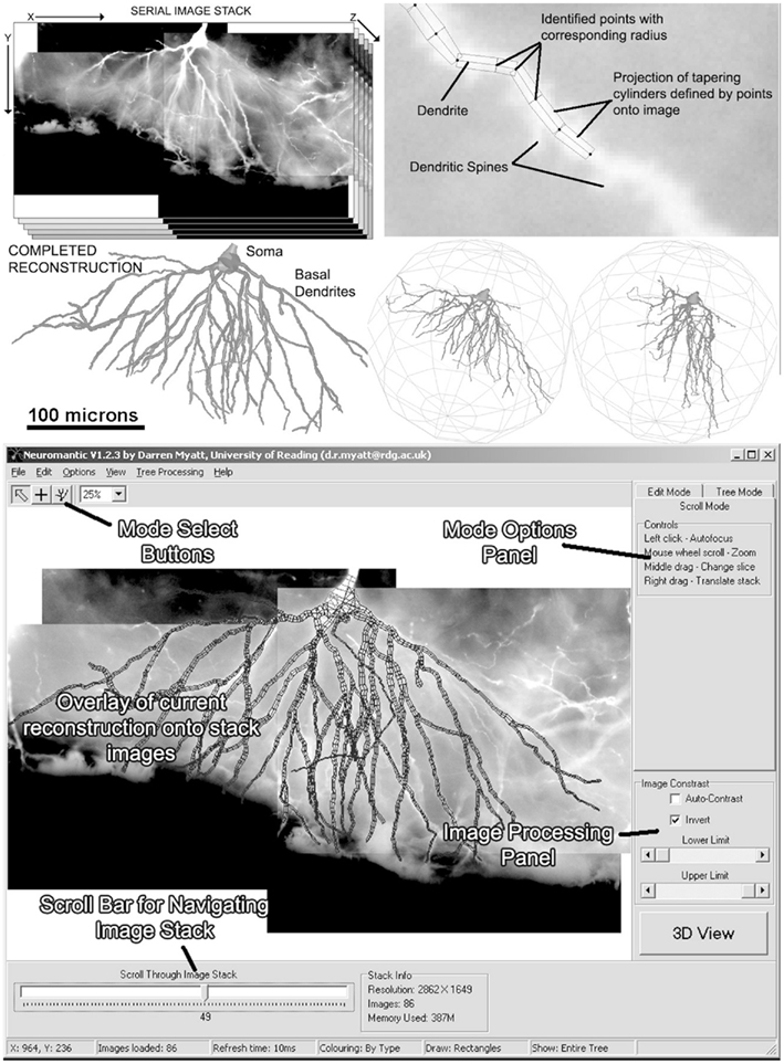
Figure 1. The process of semi-manual reconstruction and the Neuromantic application. The top panel illustrates the process of reconstruction from an image stack to a full 3D reconstruction, and the bottom panel displays the application interface with labels indicating the main features. Most of the functionality available via the interface is also replicated in mouse and keyboard shortcuts for efficiency.

Neuromantic also includes some useful real-time image processing options to aid reconstruction. With TLB stacks, where the neurites are dark on a light background, the luminosity may be inverted to allow more details to be observed in the neurites; the contrast may also be adjusted as desired through histogram stretching. These changes are only performed when drawing the visible image and do not affect the underlying stack data, thus preventing information loss.

2.1.1. Tracing algorithm

The semi-automatic reconstruction capabilities of Neuromantic are based on the LiveWire algorithm (Barrett and Mortensen, 1997; Falcao et al., 1998) for interactive segmentation of medical images, where the user selects start and end points on an image and the algorithm determines the “least cost” path between the two points. Originally designed for marking out boundaries in image data such as MRI scans, it was subsequently adapted in NeuronJ for tracing dendrites (Meijering et al., 2004) in 2D images. More recently, Meijering’s algorithm has been further automated on 2D images for estimating neurite length over a whole 2D image with multiple neurons (Zhang et al., 2007).

The algorithm uses Steerable Gaussian Filters (Freeman and Adelson, 1991) in order to identify pixels within the image stack that are likely to belong to dendrites. Additionally, it identifies the likely “flow” direction of the dendrites for each given pixel by analyzing the eigenvectors of the estimated Hessian.

Subsequently, the actual neurite path is calculated by applying Dijkstra’s graph optimization algorithm (Dijkstra, 1959) on the image pixels to find the lowest cost pixel-per-pixel route between the user-defined start and end points.

The algorithm may be readily extended to 3D (as previously implemented in other LiveWire variations for segmentation) by taking into account the new image geometry when expanding nodes. The image processing remains essentially the same, except that every image in the stack is now processed in the same way to estimate neuriteness and vector flow.

2.1.1.1. Image processing. The primary function of the image processing is to score pixels based on their likelihood that they belong to a neurite, as well as producing an estimate of the direction of each neurite for a given pixel. For the neurite tracing application, it is important for image processing to be computationally efficient, as the system needs to update fast enough for real-time user interaction. Steerable filters were therefore employed (Meijering et al., 2004), because calculating six 1-dimensional image convolutions scales linearly with respect to the number of image pixels.

Convolving the image I(x) with three linearly separable basis functions (Freeman and Adelson, 1991) produces the three basis-filtered images B_1,2,3:

where G(x) is a normalized Gaussian with standard deviation σ. From these images a Gaussianly smoothed estimate of the Hessian for pixel x is

However, following the example of Meijering et al. (2004), in this case a modified version of the Hessian is used, such that

This modified Hessian implicitly represents a more elongated version of the steerable filter. The eigenvalues and corresponding eigenvectors of the modified Hessian H^′(x) can then be used to calculate analytically the maximum response of a steerable filter at x.

The eigenvalues and eigenvectors of the modified Hessian can be calculated from those of the standard Hessian:

The measure of neuriteness, ρ(x), is calculated as

where λ(x) is the eigenvalue of the modified Hessian with the greatest absolute magnitude,

The normalizing term of λ_max in (4) is the greatest absolute eigenvalue of the correct sign over the entire image (which is negative when tracing light dendrites and positive when tracing dark dendrites). Previous work (Meijering et al., 2004; Zhang et al., 2007) has labeled this value as λ_min rather than λ_max, because only considering light dendrites on a dark background (thus referring to the negative eigenvalue with greatest magnitude). In the generalized case the use of λ_max is more intuitive.

The original equation (4) is designed to only respond to light dendrites on a dark background, such as those generated through fluorescence microscopy. The ability to follow either light or dark dendrites makes the algorithm applicable to standard transmitted light bright field and other forms of microscopy. Getting the image processing to score highly on dark dendrites instead of light can be simply achieved by changing the sign of the eigenvalues considered, in effect switching the definition of ρ(x) to

In both definitions (4) and (6), the neuriteness value is bounded such that ρ(x) ∈ [0,1].

The primary parameter affecting the estimation quality of ρ(x) is the standard deviation, σ, of the Gaussian filters. The value of σ is proportional to the radius of the dendrite that obtains maximum response with the steerable filter (Figure 2). If σ is too small compared to the radius of a given neurite then ρ(x) will become high on either side of the dendrite and low in the middle, and will effectively be perceived by the algorithm as two separate and parallel dendrites (third panel of Figure 2).

FIGURE 2

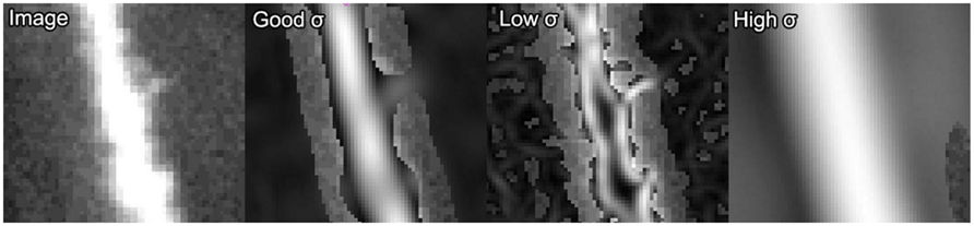
Figure 2. Example of ρ(x) response from the steerable filters for varying values of σ. From left-to-right: the original image, the ρ(x) response with an appropriate value of σ, the response with an inappropriately small value of σ and the response with an overly large σ. Areas where the original image show through indicate values of zero for ρ(x).

Conversely, a high value of σ will lead to poor tracking on thin dendrites as some curvature will be lost by the Gaussian smoothing (fourth panel of Figure 2). However, for a given value of σ, accurate traces can be made of quite a large range of dendritic radii, resulting in quite robust algorithm performance in practice.

The directional flow of the dendrite, v(x), is estimated by the eigenvector associated with the eigenvalue with the smaller absolute value.

2.1.1.2. Dijkstra routing algorithm. The Dijkstra algorithm (Dijkstra, 1959) can be used to calculate optimal routes between two given nodes on a weighted graph. It is effectively a best-first tree search, in which the node with the lowest cumulative cost is examined first at each stage.

The algorithm employs two lists, the open and closed list. The open list initially contains only the first node (or root node), which corresponds to the pixel in the image stack that the tracing will begin at, and the closed list is empty. The algorithm then proceeds as follows:

1. Take the node A with the lowest cumulative cost from the open list (or terminate if the list is empty). Move the node to the closed list.

2. Add to the open list any nodes connected to A that are not in the closed list, and calculate their cumulative cost, which is the sum of the cost of A and the cost of moving along that specific graph edge.

3. Repeat steps 1 and 2 until the desired destination node is added to the open list or the algorithm terminates unsuccessfully (if there is no route between the root node and the desired destination node).

In this way, once a given node has been considered, the optimal cost path from the source to that node is immediately known. Another useful property is that if a series of nodes x₁…x _n represent an optimal route, then a subset x₁…x _n−i (where i is a positive integer) must also be the optimal route between nodes 1 and n − i.

Extending the Dijkstra algorithm from two to three dimensions is straightforward: instead of adding just the 8 pixel-neighborhood of a pixel A to the list when A is expanded, the 9 pixels on the slices directly above and below to the open list are also added, as demonstrated in Figure 3. Even without altering the cost function, the algorithm then tends to correctly follow between slices as more in focus dendrite will have a higher neuriteness score.

FIGURE 3

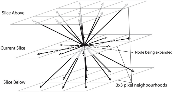
Figure 3. An illustration of how the routing algorithm is extended to 3D by adding nodes on 3 × 3 pixel neighborhoods for the slices directly above and below the specified node.

The cost function is fundamental to the neurite tracing algorithm, as it determines which overall route will be optimal. In general, the cost should be inversely related to the “likelihood” that the given pixel belongs to a neurite.

Let the vector x = {x, y, z} specify a given pixel in 3D within the image stack. The x, y coordinates specify the location within a given image, and the z coordinate specifies the stack image. Let x’ = {x, y} be the sub-vector of x containing only the x, y coordinates.

The first of the cost function terms used in Dijkstra algorithm is the neuriteness, C_λ (x), which is inversely proportional to how likely a given pixel is to belong to a neurite. The second term represents a measure of how well the current pixel-to-pixel move reflects the “flow” of the dendrite, as estimated using the eigenvectors of the Hessian matrix at that point.

Meijering’s cost function is a linear combination of these two terms, with a weighting parameter γ, and calculates the cost of moving from pixel x to y, C (x, y), as follows:

The neuriteness cost, C_λ (y), is calculated simply from the neuriteness function defined in Section 1 as

such that the cost of the pixel is inversely proportional to its neuriteness. The second term, which penalizes the movement when the neurite flow differs from the proposed pixel-to-pixel movement, is defined as

where

and

The vector flow term, C_v (x, y), is bounded in the interval 0–1, where a value of 0 indicates the pixel-to-pixel movement is completely parallel to the neurite flow on pixels x and y, and a value of 1 indicates that the movement is orthogonal to both flows.

Of the two terms, the neuriteness is considerably more important. The tracing algorithm still functions effectively when γ = 1, but completely fails as γ → 0.

Meijering’s original algorithm did not take into account normalization for diagonal pixels. The cost function for this step is multiplied by to account for the increased distance traveled compared to moving vertically or horizontally. Without this normalization the algorithm would be biased toward traveling diagonally. The diagonally corrected cost function then becomes:

For the expansion to 3 dimensions, changes in z are dealt with independently, such that if the z difference between pixels x and y is non-zero then the pixel cost is multiplied by a constant value, η. In this way, the routing may be penalized for jumping between different stack images frequently. The multiplicative z penalty, C_z (x, y), is defined as:

Integrating C_z into the above formulation yields the Neuromantic cost function:

Subsequent to optimizing pixel-by-pixel routing with the Dijkstra algorithm, the final solution is obtained by sub-sampling this route. The z value of each subsampled pixel is taken as the mean value of the pixels that make up that segment, rounded to the nearest integer.

One minor issue with strict graph optimization is that the algorithm is generally biased toward physically shorter routes (i.e., those traversing the fewest pixels). This was observed in Meijering et al. (2004), where dendrite length was consistently underestimated, although usually by a small proportion.

2.1.2. Patchwork approach

The image stacks used for this type of reconstruction can easily reach one Gigabyte in size, resulting in estimated 20 GB of RAM needed for proper operation, based on required 20 bytes per pixel and 8-bit grayscale images. Thus, image processing the entire stack would be expensive in terms of both time and space.

A practical solution to this problem is to process, in real-time, smaller patches of the image stack, rather than pre-processing the entire stack. Therefore, when the user initially clicks on the 3D start point for the dendrite, a stack of patches is added that is centered on that point (usually 128 × 128 pixels), encompassing several patches above and below the current Z coordinate (typically ±5). Overall, then, 2n + 1 patches must be analyzed, where n is the selected spread. Each patch is fully image-processed, and the neuriteness and image flow calculated and stored for each pixel, as well as sufficient memory allocated for routing information.

Neuromantic allocates new patches dynamically as the user moves the cursor along the neurite; when the mouse is moved over an area not containing a patch, a new patch stack is allocated and linked in the routing algorithms so that a trace may be created across any number of patches.

The optimal solution found using patchwork is not necessarily identical to the theoretical optimum calculated without it, although in most cases they coincide. For example, for a given set of patches, after a certain amount of processing every node in those patches will have been evaluated by the Dijkstra algorithm, leaving an empty Open list. If a new patch were added after this happened, no further routing would take place as all nodes would be already analyzed.

To avoid this problem, when a new patch is added all nodes that have already been routed to at the edge of any overlapping existing patch are re-added to the Open list, such that the routing may continue onto the new patch. However, because some nodes with a greater cost than the lowest nodes in the new patch may have already been expanded, the strict guarantee of optimality is lost. In practice, this may only have detectable effects on meandering dendrites moving from one patch to another and then back again, but it has no effect if the second patch is added before routing reaches the edge of the first one, which is the usual case.

2.2. Manual Reconstruction

An experiment was performed to examine the semi-manual reconstruction capability of Neuromantic, the time required to complete a reconstruction, and the statistical properties of these reconstructions compared with Neuron_Morpho and Neurolucida reconstructions of the same neuron.

The trial consisted of ten participants (postgraduate student volunteers at the University of Reading’s), each of whom reconstructed the basal dendrites of a CA1 rat hippocampal neuron (as described in Section 4).

All the participants worked with a luminosity-inverted version of the stack as the dendrite details were more apparent. They were also able to alter the contrast to highlight branches more effectively, but advised to keep it at one setting throughout the reconstruction.

Participants were given step-by-step instructions for adding new segments and branch points, and example images of how correctly segmented branches should look, enabling more effective identification, and tracing of dendrites with high spine density.

2.3. Semi-Automatic Reconstruction

The key to routing algorithm accuracy is the quality of its cost function. The cost function should be monotonically decreasing with increasing likelihood that the pixel belongs to a neurite.

We examined the effect of applying exponential function to the cost terms on the tracing quality. Integer exponents were selected because they would help penalize areas with low neuriteness and help reduce the incidence of shortcuts taken over non-neurite pixels. Also, they are highly efficient to compute, so the speed of the algorithm would not be significantly reduced.

The considered cost function is generalized to

where a and b are non-negative integers.

The original cost function is a specific case of the generalized function where a = 1, b = 1. The quality of tracing was explored for several values of a and b over a variety of neuronal tracing tasks, and the accuracy of the tracings compared to a carefully hand-segmented reconstruction.

2.3.1. Error metrics

Two main metrics were used in order to assess reconstruction accuracy – midline tracking (considering x, y) and depth error (considering z), (Myatt et al., 2006). The z axis was treated separately because the z axis is qualitatively different from the x/y axis in many microscopy techniques, particularly light microscopy. It is typical for the z resolution of the image stack to be significantly lower than the x, y resolution.

Let the series of 3D points representing the ground-truth be ω_1…n, where ω_i= {x, y, z}. Similarly, the estimated reconstruction is A piece-wise linear model of the estimated dendrite midline can then be generated by connecting straight segments between the specified 3D coordinates of and for j = 1…m − 1.

For each of the ground-truth segment points, ω_i, the closest point along this piece-wise linear midline may be determined: the parameters of that point, are assumed to be a linear combination of the parameters of the two segment points that defined it, and such that

where α ∈ [0, 1] was the proportional distance along the line. This allows the estimation of a value of the z coordinate at this point, although individual z values for each point are rounded to the nearest integer. The errors are then calculated based on parameter differences between ω_i and

Midline tracking error is the error, in pixels, from the x, y positions defined by ω_i and

Depth error is the error, in slices, between the depths defined by ω_i and Both depths are rounded to the nearest integer value, as the original hand segmentation is only accurate to ±0.5 slices.

2.3.2. Experiments varying cost function

Eight different cost functions combining different polynomial terms of the neuriteness and neurite flow were examined to investigate neurite tracing accuracy:

where N represents the neuriteness term C_λ (y) and V the vector flow term. The first condition of N alone was added to verify the necessity of the vector flow term, as it has a much less significant effect than the neuriteness term. The second condition represents the original cost function.

A z penalty multiplier of η = 1.3 was selected. The cost function, informed by the default setting in NeuronJ, was substantially biased toward the neuriteness term with γ = 0.9.

For comparison, the final paths were subsampled by a factor of 5.

2.3.3. Significance testing

To be recommended, a given cost function variant must perform significantly better than the standard function N + V. The performance of each cost function on all benchmark neurites was ranked applying Wilcoxon rank sum test (Wilcoxon, 1945) with significance level α = 0.05.

The Bonferroni correction for multiple comparisons was applied (Miller, 1991), to minimize spurious significant results. This overly conservative approach increases the false negative probability, as the different costs functions are not truly independent.

The null hypothesis, H₀, is that there is no significant consistent difference between the tracing quality produced by different cost functions, whereas the alternative hypothesis is that the cost function has some consistent effect on tracing quality.

In the case of testing the varying values of η, each other value will be compared against a value of η = 1.0, as this represents the default case of no biasing for moving between different image slices.

2.4. Data

The benchmark data used to evaluate manual reconstruction as well as semi-automatic tracking came from 200 μm brain sections from adult, male, Sprague-Dawley rats (Desmond et al., 1990) stained using a modified rapid-Golgi method (Desmond and Levy, 1982). A manually selected CA1 pyramidal neuron from hippocampal CA1 area was imaged using an Olympus BX51 microscope with an Olympus Arch x60 dry objective. The resulting image set consists of 5 stacks stitched together using the Volume Integration and Alignment System (VIAS) freeware software (Rodriguez et al., 2003). Every stack contains 86 images, each with a resolution of 2862 × 1649. Using 8-bit color depth, the total memory required to hold the stack is 387 MB.

The original Neuron_Morpho and Neurolucida reconstructions from (Brown et al., 2005) were kindly made available to us. To constrain the duration of experiments, only the basal tree was considered. The two original reconstructions were therefore edited in Neuromantic to remove their apical dendrites. This can be achieved easily in Neuromantic by holding down the ALT key and clicking on any apical dendritic segment, selecting all apical dendrites. Pressing delete will then remove all such segments. Of these edited reconstructions, the Neuron_Morpho basal tree had 2573 segments, and the Neurolucida reconstruction 2258 segments.

For the semi-automatic reconstruction experiments five branches were selected as benchmarks and manually reconstructed by the first author to obtain the ground-truth against which the semi-automatic reconstruction could be assessed.

The second set of benchmarks for semi-automatic reconstruction comes from a guinea pig piriform cortex neuron labeled with Neurobiotin, (Libri et al., 1994) and imaged with a Nikon Eclipse E1000 with a Nikon x20 dry objective in a single field of view, with a z resolution of 0.8 μm. The image stack has a resolution of 3840 × 3072 pixels, and contains 99 slices. This neuron had undergone significant deformation from shrinkage during histology, yielding highly meandering dendritic paths: although an artifact, these dendrites are very difficult to trace due to both the low contrast and shape, and thus represent a very challenging benchmark. The dendrites frequently double back on themselves, meaning that it is exceedingly easy for a tracing algorithm to miss sections by jumping from one part to another.

Five branches were carefully segmented using the semi-manual capabilities of Neuromantic as test cases. Analogously to Meijering et al. (2004), the midline was identified while using a highly zoomed version of the stack with bicubic image interpolation enabled to maximize accuracy.

Example images from the two benchmark stacks are shown in Figure 4, along with the ten selected test dendrites.

FIGURE 4

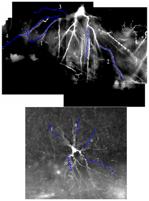
Figure 4. An example image from both benchmark image stacks, with the position of the ten benchmark dendrites marked upon them. The luminosity is inverted in both cases (the stacks are naturally dark dendrites on a light background), and the luminosity histogram has been stretched to improve the contrast with the background.

3. Results

The number of reconstructed segment per time produced by participants varied from 861 and 4549, and the overall time taken from 140 to 290 min. The segments added per minute ranged from 4.5 to 15.7, with a mean value of 10.2. For comparison, Brown et al. (2005) reported that each entire pyramidal neuron took approximately 20 h (1200 min) to reconstruct with both applications. Therefore the Neurolucida reconstruction (with 5759 segments) yielded approximately 4.8 segments/min, whereas the Neuron_Morpho reconstruction (with 7499 segments) gave 6.2 segments/min.

The number of segments per time is used here as an index indicative of the ease of use of reconstruction software, eliminating variations due to the average segment length. However, it is worth noting that the amount of segments in semi-manual reconstructions produced by each participant varied significantly, despite the fact that the introductory demonstration included a recommended segment size in order to reduce this issue. This is mainly attributed to the varying desire of the participants to complete the task as quickly as possible, and seems unavoidable in a trial of this kind without imposing some physical segment length limit within the software itself.

A variety of statistical measures from the reconstructions were calculated using L-Measure (Scorcioni et al., 2008).

3.1. Morphological Comparison of Reconstructions

Figure 5 shows a rendering of the ten reconstructions generated by the participants in the experiment, along with the cut-down Neuron_Morpho and Neurolucida reconstruction. The basic morphology is similar for each, although there is significant variance with respect to the presence of the smaller branches.

FIGURE 5

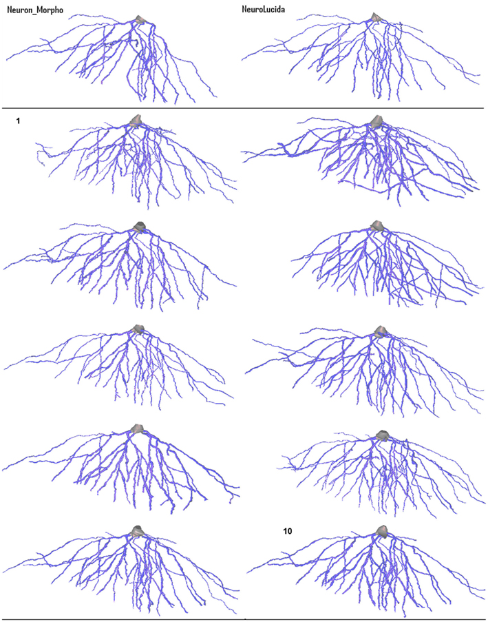
Figure 5. Variation in morphology of the 10 basal tree reconstructions created by the participants in the experiment (they are in ascending order from left-to-right). The Neuron_Morpho reconstructions and Neurolucida reconstructions presented in Brown et al. (2005) are shown to allow visual comparison.

The most obvious gross morphological difference between the Neuron_Morpho and Neurolucida reconstructions is that the former lacks the large branch furthest to the right. All Neuromantic reconstructions contain at least part of this branch.

Significant variation in radius estimation can be clearly seen over the reconstructions: visually reconstruction 5 appears to have the thinnest dendrites (closest to the original Neurolucida reconstruction). Reconstruction 2, on the other hand, demonstrates the widest dendrites, and should therefore have the largest overall volume and surface area. These observations are confirmed by the statistical analysis.

3.2. Statistical Analysis of Reconstructions

Segment data were post-processed in order to remove obvious reconstruction errors (e.g., tracing an obvious length of axon rather than dendrite, tracing a wildly out-of-focus dendrite, initiation of the reconstructions at different points on the soma). This resulted in minor discrepancy between the numbers of segments used for calculation of speed of reconstruction (original raw numbers of segments used in Table 1) and the number of segments used for calculating dendritic tree statistics (Tables 2 and 3). However, this difference had a negligible effect on the considered dendritic branch statistics.

TABLE 1

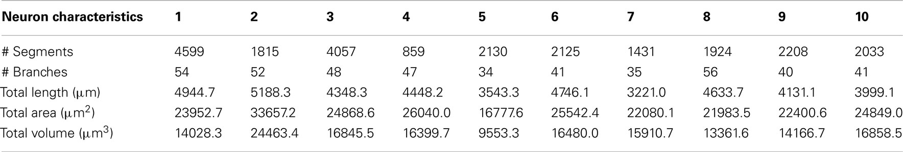
Table 1. Gross neuron statistics for each of the ten reconstructions created by the participants.

TABLE 2

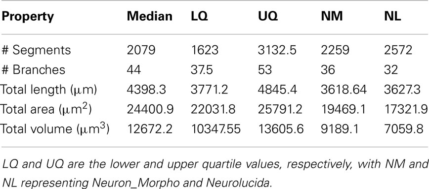
Table 2. The median and interquartile range of the experimental reconstructions compared to the Neuron_Morpho and Neurolucida reconstructions.

TABLE 3

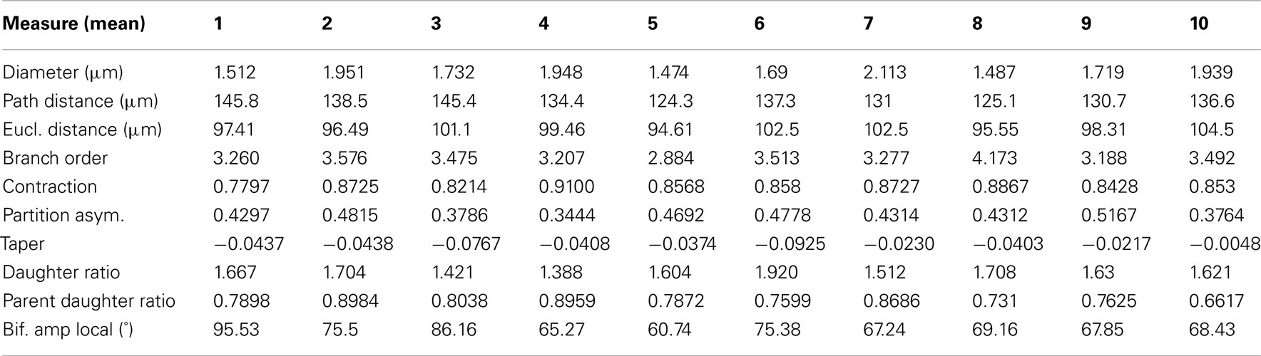
Table 3. The mean branch statistics for each of the ten reconstructions performed by the participants.

3.2.1. Gross neuron statistics

The total reconstructed dendritic surface area and volume, defined as the sum over all segments of respectively, segment surface and volume, were based on the assumption that each segment is a uniform cylinder (as opposed to a tapering one), Table 1.

The interquartile range for overall volume is around 3000 μm³, which is about 25% of the median value. However, such variation is not unexpected, as other investigations into inter-user variance on different systems have consistently found very significant variation between both different operators on the same system and the same operator on different systems (Jaeger, 2000; Kaspirzhny et al., 2002). The interquartile range for overall surface area is approximately 4000μm² (17% of the median value); consistent with the volume being quadratic function of the radius, rather than a linear one (as with surface area).

The variations in the quality of a reconstruction come from two major sources: the number of identified and segmented branches, and the quality of the segmentation of each branch (midline and radius estimation). Some gross properties, such as the total number of branches, are only attributable to one of these factors (branch identification), whereas the overall volume, for example, is a function of both.

The measurement of the dendritic radius contributing to the quality of branch segmentation is always the most variable aspect of neuronal reconstructions: due to the integration of the image volume with the Point Spread Function the edges between the dendrites and the background are blurred, and thus the choice of diameter tends to be subjective. Estimation of radii can vary significantly between different labs performing neuronal reconstruction (Scorcioni et al., 2004).

For this experiment, participants were instructed to estimate the dendrite edge as where the brightest luminosity of the pixels first began to decrease (since the participants were working with a luminosity-inverted stack, the dendrites were lighter than the background). On the other hand, the reconstruction procedure used in (Brown et al., 2005) in Neuron_Morpho and Neurolucida employed a measuring scheme of 4 pixels on either side of the darkest pixels. Consequently, one has to be cautious not to draw quantitative conclusions when comparing the relative volumes of the reconstructions.

Table 2 shows the median and interquartile range over all reconstructions for the metrics in Table 1.

In summary, these data suggest that the Neuromantic interface makes it simple to navigate the image data and identify dendrites that have not yet been segmented. This might be due to the use of an inverted image stack making dendritic details clearer or the variety of options available for overlaying the current reconstruction.

3.2.2. Branch statistics

Table 3 contains the mean value of branch statistics for all the reconstructions, whereas Table 4 shows the median and lower/upper quartiles over all reconstructions, along with the corresponding Neurolucida/Neuron_Morpho values for comparison.

TABLE 4

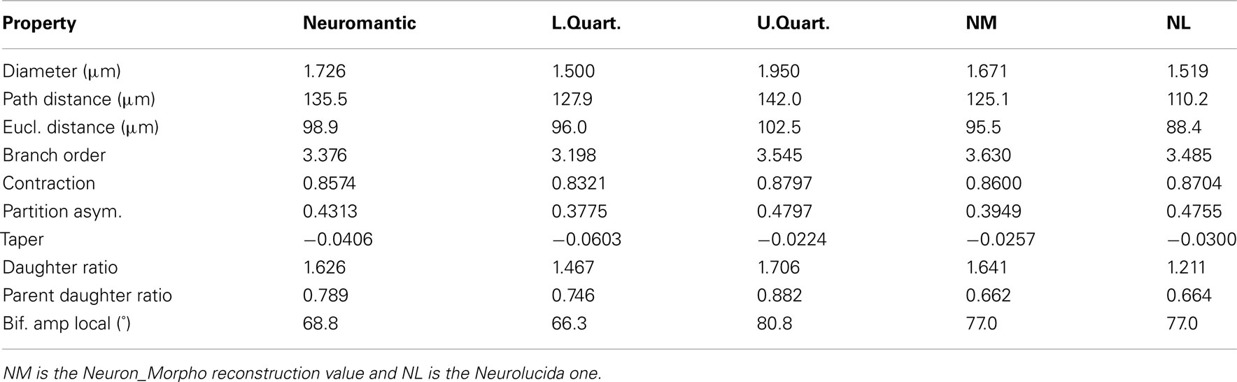
Table 4. The median and interquartile branch statistics for each of the ten reconstructions performed by the participants.

The mean diameter of the Neuron_Morpho and Neurolucida reconstructions falls within the interquartile range observed in the experiment (0.45 μm), with the proportional difference between the median and the original reconstructions being just over 10% at maximum.

The median path, and Euclidean mean, distances for branches, however, do not fall within 10% of either the Neurolucida or Neuron_Morpho reconstructions reflecting the generally larger number of branches identified by the participants.

Contraction (always between 0 and 1) is a measure of dendritic meandering, with 1 indicating perfectly straight dendrites and decreasing values increasing “wiggle.” The interquartile range of the experimental contraction values (≈0.05) encompasses the associated values of both original reconstructions. The median value observed in the experiment is also within <5% of both the original values.

For the partition asymmetry, the Neuron_Morpho and Neurolucida values again lie within the experimental interquartile range, and the median within <10% of both values. Interestingly, though, the Neuron_Morpho and Neurolucida values differ significantly by around <20% on this metric; likely attributable to the missing right hand branch in the Neuron_Morpho reconstruction (Figure 5). Also, partition asymmetry, like branch order, is somewhat sensitive to the presence/absence of minor branches.

The taper measure used here is the mean decrease in diameter per unit length. The experimental reconstructions tended to have greater mean taper rates than the original reconstructions, and the interquartile range of this metric was large at 0.04.

The daughter ratio is the ratio of the radius of the wider daughter branch from a bifurcation to the thinner branch (and thus is always ≥1). Here, a large difference is observed between the Neuron_Morpho and Neurolucida reconstructions (1.64 and 1.21, respectively), with the Neuromantic interquartile range encompassing the Neuron_Morpho value but not the Neurolucida one, and the Neuromantic median being highly similar to the Neuron_Morpho value (at 1.63). It is possible that the differing interfaces bias operators into segmenting bifurcations in different ways, and Neuromantic’s basic method for semi-manual reconstruction is much more similar to Neuron_Morpho than Neurolucida’s.

As for the parent daughter ratio (the diameter of the daughter branch divided by that of the parent branch), the interquartile range includes neither the Neuron_Morpho nor the Neurolucida reconstructions. This may be partly due to a tendency for the inexperienced participants to systematically overestimate the radius leading to larger parent daughter ratio scores.

The local bifurcation angles measured in the experiment were also significantly different than the original reconstructions. The Neuron_Morpho and Neurolucida values were both highly similar (with less than a degree’s difference), and are encompassed by the experimental interquartile range (≈14°). As the bifurcation angle is only calculated based upon the angle between the parent and daughter segments, there is significant scope for subjective difference as to the parent segment placement.

Both of the original reconstructions were segmented by the same individual, thus minimizing subjective inter-user differences. Therefore, it is to be expected that the Neuron_Morpho and Neurolucida reconstructions would be more similar to each other than to Neuromantic ones.

Some of the reconstruction variability may be attributed to the fact that the participants were non-experts, hence reflecting some of the participants’ incorrect understanding of the actual task, rather than issues with the application itself (based on a short debriefing session afterward). Each participant increased in speed over the course of the experiment as they became more used to visually interpreting the image stacks and repeating the basic process of segmenting the neurons.

3.3. The effect of cost function on tracing accuracy

The results reported illustrate the effect of modifying the cost function on the x/y tracking. The corresponding effect on z tracking, was examined but found negligible (results not shown).

Table 5 shows the mean square x/y tracking error (as defined in Section 1) for each cost function over all ten benchmarks.

TABLE 5

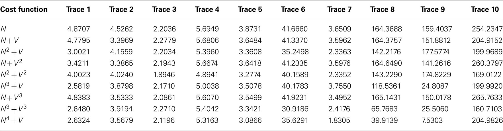
Table 5. The mean square x/y tracking error for each of the ten benchmark problems over all nine cost functions.

Significant variation is observed between cost functions. Particularly, much larger errors are seen in the second set of benchmarks 6–10, as it is possible for the routing algorithms to miss out significant sections of the neurite because of their meandering nature. Figure 6 shows typical shortcut errors made when tracing benchmark 10.

FIGURE 6

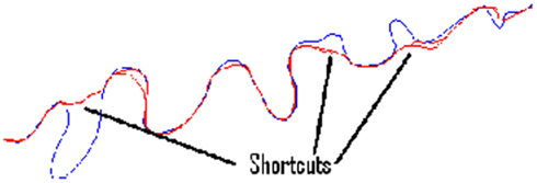
Figure 6. The ground-truth tracing for benchmark neurite 10 (rotated 90° anticlockwise), along with examples of the tracing errors caused by taking shortcuts.

Table 6 displays the mean (ascending x/y tracking error) ranking of each cost function over all ten benchmarks. The Bonferroni corrected value of α is 0.05/8 = 0.0063, implying statistical significance for the N⁴ + V cost function. However, 4 out of the 8 alternative cost functions had p-values lower than 0.05. The likelihood of such an event occurring by chance is 0.037%, so some Type II errors (false negatives) have probably been made. In general, though, cost functions with a neuriteness exponent of greater than one are likely providing real and consistent improvements, whereas changes to the vector flow exponent are insignificant.

TABLE 6

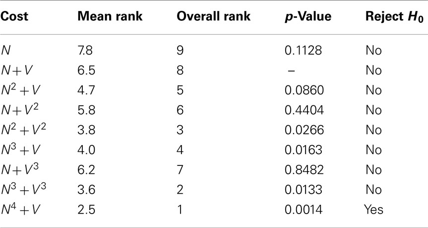
Table 6. The mean quality ranking for each cost function based on x/y tracking alone, as well as the p-values obtained from statistical testing.

As expected, the neuriteness term exponent, a, is significantly more important than the associated vector flow exponent b. Increasing the vector flow exponent improves quality on x/y tracking to a much lesser extent, consistently with the neuriteness being the most significant term in the cost function. Therefore, these results indicate that cost functions using higher exponents are generally to be preferred for x/y tracking to the original cost function N + V.

Table 7 shows the effect on the overall length estimation of the benchmark dendrite as a result of varying the cost function.

TABLE 7

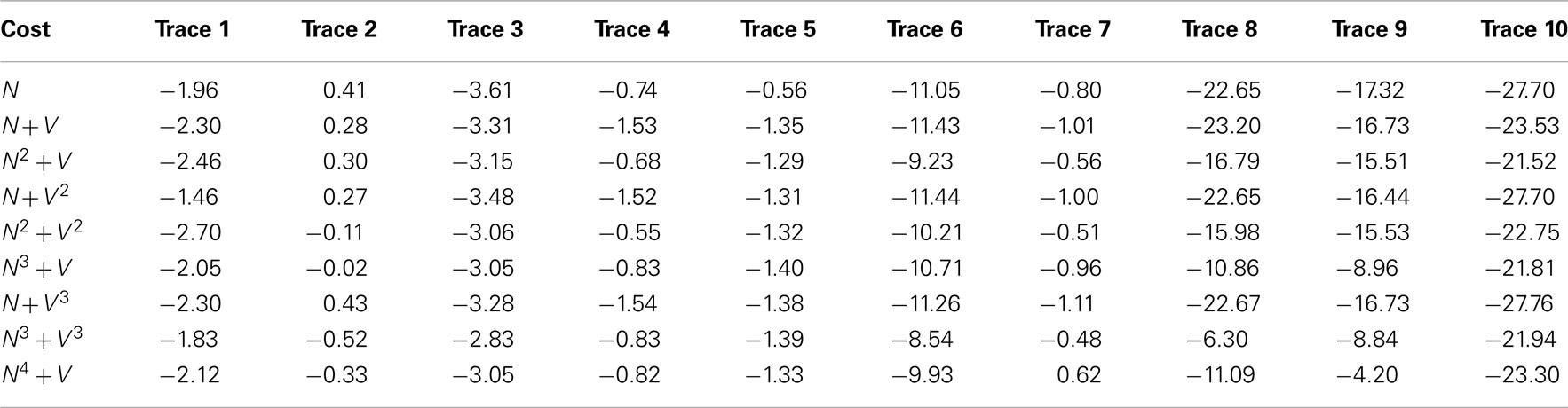
Table 7. The percentage length errors over the benchmarks as a result of varying the cost function associated with the routing algorithm.

As expected from previous work, the actual length tends to be underestimated, due to Dijkstra’s algorithm preference for physically shorter routes. For the normal dendrites (benchmarks 1–5), though, the errors tend to be consistently less than 4% of the overall length. When considering the meandering dendrites, however, the length estimation errors are generally much larger, sometimes up to 20% of the overall length, which is much less acceptable and would have a very significant effect on simulation if left uncorrected. Such large errors, as explained previously in relation to x/y tracking, result from the routing taking shortcuts over tight curves. However, this tracing algorithm is part of a semi-automatic method, and errors of this magnitude are trivial to spot visually and account for when performing the tracing. Thus, smaller values are still preferable as they mean less user intervention.

4. Conclusion

Neuromantic is a freeware application for producing three dimensional reconstruction of neurons. Its performance was demonstrated in manual and semi-automated reconstructions from non-deconvolved Transmitted Light Brightfield (TLB) image stacks. In these cases, lighting intensity varies across the image, making the data unsuitable for global thresholding to segregate dendrites from background. Also, the numerous out-of-focus artifacts mean that the data is not a true 3D voxel representation of the neuron. Significantly more image processing is thus required than for confocal stacks to extract accurate neuronal morphology.

Non-deconvolved stacks were considered, as effective deconvolution is often difficult on Golgi stained or Biocytin labeled and stained stacks. However, Neuromantic may be applied equally well to the reconstruction of dendrites from deconvolved image stacks.

The application was compared to a similar freeware system, Neuron_Morpho, and a commercially available package, Neurolucida, indicating comparable speed of use and inter-user variation consistent with that reported for other comparable studies.

Our informal survey of Neuromantic users indicates appreciation of its lightweight feel and simple interface for basic visualization and editing. The ability of dynamic image loading offers possibility to work smoothly with very large image stacks with moderate and widely available computer platforms. Semi-automated reconstruction from any given point requires simply clicking on an existing point and tracing the branch without the need, common in other systems, to open context menus to label points. Similarly, the diverse and user-friendly options of automated point selection, offer a quick way of investigating alternative reconstructions which often require modification of already completed reconstructions. For example, Neuromantic enables easy connectivity changes and immediate visual edits. Both operations require cvapp (Cannon et al., 1998) when working with Neuron_Morpho. Such features, over long usage term, may save hundreds of labor hours. Although other systems offer 3D visualization of the underlying image stack (Rodriguez et al., 2003), Neuromantic efficient memory management yields smoother manipulation of large stacks, whereas more sophisticated programs may struggle on computers with standard graphics card.

The perceived optimal trade-off between utility and ease of learning was also a factor that motivated the selection of Neuromantic as the official editing tool in the DIADEM challenge (diademchallenge.org). Neuromantic was also adopted by the DIADEM organizers to prepare the challenge data (Brown et al., 2011) and test the scoring metric (Gillette et al., 2011a). The results of DIADEM highlighted a need for a user-friendly editing and visualization platform, which Neuromantic fills in this regard (Peng et al., 2011). Moreover, the open source release of Neuromantic allows developers to combine this interface and algorithm with the advances that resulted from DIADEM competition and other recent developments (Donohue and Ascoli, 2011).

To address the known problems with inter-user variance on semi-manual reconstructions, the Neuromantic 3D image stacks extension to semi-automatic tracing (Meijering et al., 2004) was introduced. In order to mitigate the computational effort and memory requirements when tracing dendrites through large stacks of high-resolution images, the semi-automated tracing employs patchwork representation of the image, processing, routing, and allocating data dynamically during the user interaction.

The method was evaluated in terms of reconstruction consistency, examining the effect of the routing algorithm’s cost function form on the accuracy of dendrite midlines over a range of benchmarks. Increasing the exponents of the cost function two terms significantly improved tracing quality. The term relating to the likelihood of a given pixel belonging to a dendrite was significantly more important than the term relating to directional flow.

The modification to the Dijkstra cost function, suggested by these results, produced a consistent improvement in tracing accuracy, allowing the application to automatically deal with more complex cases such as meandering dendrites. Furthermore, it also reduced required user interaction, thus decreasing the overall time needed to generate accurate 3D neuronal models.

The semi-automatic mode uses just three parameters of which only one (the standard deviation of the steerable Gaussian) requires adjustment based on the widths of reconstructed dendrites, with minimal effect on reconstruction quality, while default value of the remaining two parameters provide overall accurate reconstructions. The small number of parameters and ease of their setting is consistent with recently recommended good practice in neurite reconstruction algorithm design (Meijering, 2010). Although other systems (e.g., those presented at the DIADEM competition) offer higher levels of automation, the semi-automatic capability of Neuromantic certainly enhance its user friendliness.

To conclude, Neuromantic is suggested as a useful open source tool for reconstructing dendritic trees. It provides great flexibility and a good balance between speed of operation and resultant quality. Neuromantic thus is a useful addition to the repertoire of available tools for neuronal reconstruction that might appeal to some researchers.

Conflict of Interest Statement

The authors declare that the research was conducted in the absence of any commercial or financial relationships that could be construed as a potential conflict of interest.

Acknowledgments

This work was supported by EPSRC Grant GR/S55897/01 and EP/F033036/1 to Slawomir J. Nasuto. Giorgio A. Ascoli acknowledges support from NIH R01 NS39600. We thank Kerry Brown for providing the TLB image stack used in this paper as a benchmark, as well as the Neurolucida and Neuron_Morpho reconstructions. Furthermore, we thank Nancy Desmond for providing the sample containing the rat hippocampal sample, and Andy Constanti for donating the guinea pig piriform cortex sample.

Footnotes

1. ^DiademChallenge.Org
2. ^sourceforge.net/p/neuromantic

References

Ascoli, G. A. (2006). Mobilizing the base of neuroscience data: the case of neuronal morphologies. Nat. Rev. Neurosci. 7, 318–324.

Pubmed Abstract | Pubmed Full Text | CrossRef Full Text

Ascoli, G. A., Donohue, D., and Halavi, M. (2007). NeuroMorpho.Org – A central resource for neuronal morphologies. J. Neurosci. 27, 9247–9251.

Pubmed Abstract | Pubmed Full Text | CrossRef Full Text

Ascoli, G. A., Krichmar, J., Scorcioni, R., Nasuto, S. J., and Senft, S. (2001). Computer generation and quantitative morphometric analysis of virtual neurons. Anat. Embryol. 204, 283–301.

Pubmed Abstract | Pubmed Full Text | CrossRef Full Text

Barrett, W. A., and Mortensen, E. N. (1997). Interactive live-wire boundary extraction. Med. Image Anal. 1, 331–341.

Pubmed Abstract | Pubmed Full Text | CrossRef Full Text

Bas, E., and Erdogmus, D. (2011). Principal curves as skeletons of tubular objects: locally characterizing the structures of axons. Neuroinformatics 9, 181–191.

Pubmed Abstract | Pubmed Full Text | CrossRef Full Text

Brown, K. M., Barrionuevo, G., Canty, A. J., De Paola, V., Hirsch, J. A., Jefferis, G. S., Lu, J., Snippe, M., Sugihara, I., and Ascoli, G. A. (2011). The DIADEM data sets: representative light microscopy images of neuronal morphology to advance automation of digital reconstructions. Neuroinformatics 9, 143–157.

Pubmed Abstract | Pubmed Full Text | CrossRef Full Text

Brown, K. M., Donohue, D. E., D’Alessandro, G., and Ascoli, G. A. (2005). A cross-platform freeware tool for digital reconstruction of neuronal arborizations from image stacks. Neuroinformatics 3, 343–359.

Pubmed Abstract | Pubmed Full Text | CrossRef Full Text

Cannon, R. C., Turner, D. A., Pyapali, G. K., and Wheal, H. V. (1998). An on-line archive of reconstructed hippocampal neurons. J. Neurosci. Methods 84, 49–54.

Pubmed Abstract | Pubmed Full Text | CrossRef Full Text

Chothani, P., Mehta, V., and Stepanyants, A. (2011). Automated tracing of neurites from light microscopy stacks of images. Neuroinformatics 9, 263–278.

Pubmed Abstract | Pubmed Full Text | CrossRef Full Text

Denk, W., Strickler, J. H., and Webb, W. W. (1990). Two-photon laser scanning fluorescence microscopy. Science 248, 73–76.

Pubmed Abstract | Pubmed Full Text | CrossRef Full Text

Desmond, N. L., Heydenreich, M. S., and Levy, W. B. (1990). Quantitative characterization of the hippocampal CA1 pyramidal cell dendritic field in stratum moleculare. Anat. Rec. 226, 26A.

Desmond, N. L., and Levy, W. B. (1982). A quantitative anatomical study of the granule cell dendritic fields of the rat dentate gyrus using a novel probabilistic method. J. Comp. Neurol. 212, 131–145.

Pubmed Abstract | Pubmed Full Text | CrossRef Full Text

Dijkstra, E. (1959). A note on two problems in connexion with graphs. Numer. Math. 1, 269–270.

CrossRef Full Text

Donohue, D., and Ascoli, G. A. (2011). Automated reconstruction of neuronal morphology: an overview. Brain Res. Rev. 67, 94–102.

Pubmed Abstract | Pubmed Full Text | CrossRef Full Text

Falcao, A. X., Udupa, J. K., Samarasekera, S., and Sharma, S. (1998). User-steered image segmentation paradigms: live wire and live lane. Graph. Models 60, 233–260.

CrossRef Full Text

Freeman, W. T., and Adelson, E. H. (1991). The design and use of steerable filters. IEEE Trans. Pattern Anal. Mach. Intell. 13, 891–906.

CrossRef Full Text

Gillette, T. A., Brown, K. M., and Ascoli, G. A. (2011a). The DIADEM metric: comparing multiple reconstructions of the same neuron. Neuroinformatics 9, 233–245.

CrossRef Full Text

Gillette, T. A., Brown, K. M., Svoboda, K., Liu, Y., and Ascoli, G. A. (2011b). DIADEMchallenge.Org: a compendium of resources fostering the continuous development of automated neuronal reconstruction. Neuroinformatics 9, 303–304.

CrossRef Full Text

Jaeger, D. (2000). “Accurate reconstruction of neuronal morphology,” in Computational Neuroscience: Realistic Modeling for Experimentalists, ed. E. De Schutter (Boca Raton: Lewis Publishers, Inc.), 159–178.

Kaspirzhny, A. V., Gogan, P., Horcholle-Bossavit, G., and Tyc-Dumont, S. (2002). Neuronal morphology data bases: morphological noise and assessment of data quality. Network 13, 357–380.

Pubmed Abstract | Pubmed Full Text | CrossRef Full Text

Kaufmann, E. W., and Moser, W. H. (2000). Dendritic anomalies in disorders associated with mental retardation. Cereb. Cortex 10, 981–991.

Pubmed Abstract | Pubmed Full Text | CrossRef Full Text

Libri, V., Constanti, A., Calaminici, M., and Nistic, G. (1994). A comparison of the muscarinic response and morphological properties of identified cells in the guinea-pig olfactory cortex in vitro. Neuroscience 59, 331–347.

Pubmed Abstract | Pubmed Full Text | CrossRef Full Text

Liu, Y. (2011). The DIADEM and beyond. Neuroinformatics 9, 99–102.

Pubmed Abstract | Pubmed Full Text | CrossRef Full Text

Lu, J. (2011). Neuronal tracing for connectomic studies. Neuroinformatics 9, 159–166.

Pubmed Abstract | Pubmed Full Text | CrossRef Full Text

Meijering, E. (2010). Neuron tracing in perspective, cytometry part A. 77A, 693–704.

Meijering, E., Jacob, M., Sarria, J. C. F., Steiner, P., Hirling, H., and Unser, M. (2004). Design and validation of a tool for neurite tracing and analysis in fluorescence microscopy images. Cytometry 58A, 167–176.

Miller, R. G. Jr. (1991). Simultaneous Statistical Inference. New York: Springer-Verlag.

Myatt, D. R., Nasuto, S. J., and Maybank, S. J. (2006). “Towards the automatic reconstruction of dendritic trees using particle filters,” in Proceedings of Nonlinear Statistical Signal Processing Workshop 2006 (on CD-ROM), Cambridge.

Narayanaswamy, A., Wang, Y., and Roysam, B. (2011). 3-D image pre-processing algorithms for improved automated tracing of neuronal arbors. Neuroinformatics 9, 219–231.

Pubmed Abstract | Pubmed Full Text

Nasuto, S. J., Knape, R., Krichmar, J. L., and Ascoli, G. A. (2001). Relation between neuronal morphology and electrophysiology in the Kainate lesion model of Alzheimer’s Disease. Neurocomputing 38–40, 1477–1487.

CrossRef Full Text

Peng, H., Long, F., Zhao, T., and Myers, E. (2011). Proof-editing is the bottleneck of 3D neuron reconstruction: the problem and solutions. Neuroinformatics 9, 103–105.

Pubmed Abstract | Pubmed Full Text | CrossRef Full Text

Rodriguez, A., Ehlenberger, D., Kelliher, K., Einstein, M., Henderson, S. C., Morrison, J. H., Hof, P. R., and Wearne, S. L. (2003). Automated reconstruction of three-dimensional neuronal morphology from laser scanning microscopy images. Methods 30, 94–105.

Pubmed Abstract | Pubmed Full Text | CrossRef Full Text

Ropireddy, D., Scorcioni, R., Lasher, B., Buzsáki, G., and Ascoli, G. (2011). Axonal morphometry of hippocampal pyramidal neurons semi-automatically reconstructed after in-vivo labeling in different CA3 locations. Brain Struct. Funct. 216, 1–15.

Pubmed Abstract | Pubmed Full Text | CrossRef Full Text

Scorcioni, R., Lazarewicz, M. T., and Ascoli, G. A. (2004). Quantitative morphometry of hippocampal pyramidal cells: differences between anatomical classes and reconstructing laboratories. J. Comp. Neurol. 473, 177–193.

Pubmed Abstract | Pubmed Full Text | CrossRef Full Text

Scorcioni, R., Polavaram, S., and Ascoli, G. A. (2008). L-Measure: a web-accessible tool for the analysis, comparison and search of digital reconstructions of neuronal morphologies. Nat. Protoc. 3, 866–876.

Pubmed Abstract | Pubmed Full Text | CrossRef Full Text

Senft, S. L. (2011). A brief history of neuronal reconstruction. Neuroinformatics 9, 119–128.

Pubmed Abstract | Pubmed Full Text | CrossRef Full Text

Svoboda, K. (2011). The past, present and future of single neuron reconstruction. Neuroinformatics 9, 97–98.

Pubmed Abstract | Pubmed Full Text | CrossRef Full Text

Türetken, E., González, G., Blum, C., and Fua, P. (2011). Automated reconstruction of dendritic and axonal trees by global optimization with geometric priors. Neuroinformatics 9, 279–302.

Pubmed Abstract | Pubmed Full Text | CrossRef Full Text

van Elburg, R. A. J., and van Ooyen, A. (2010). Impact of dendritic size and dendritic topology on burst firing in pyramidal cells. PLoS Comput. Biol. 6, e1000781. doi:10.1371/journal.pcbi.1000781

CrossRef Full Text

Wang, Y., Narayanaswamy, A., Tsai, C. L., and Roysam, B. (2011). A broadly applicable 3-D neuron tracing method based on open-curve snake. Neuroinformatics 9, 193–217.

Pubmed Abstract | Pubmed Full Text | CrossRef Full Text

Whalley, B. J., Postlethwaite, M., and Constanti, A. (2005). Further characterization of muscarinic agonist-induced epileptiform bursting activity in immature rat piriform cortex, in vitro. Neuroscience 134, 549–566.

Pubmed Abstract | Pubmed Full Text | CrossRef Full Text

Wilcoxon, F. (1945). Individual comparisons by ranking methods. Biometrics 1, 80–83.

CrossRef Full Text

Zhang, Y., Zhou, X., Degterev, A., Lipinski, M., Adjeroh, D., Yuan, J., and Wong, S. T. C. (2007). Automated neurite extraction using dynamic programming for high-throughput screening of neuron-based assays. Neuroimage 35, 1502–1515.

Pubmed Abstract | Pubmed Full Text | CrossRef Full Text

Zhao, T., Xie, J., Amat, F., Clack, N., Ahammad, P., Peng, H., Long, F., and Myers, E. (2011). Automated reconstruction of neuronal morphology based on local geometrical and global structural models. Neuroinformatics 9, 247–261.

Pubmed Abstract | Pubmed Full Text | CrossRef Full Text