Neuronvisio: a graphical user interface with 3D capabilities for NEURON

1. Introduction

While it is possible to formalize a set of differential equations to model a neuron or a neuronal network, the complexity of such a task becomes more daunting as the models become larger. Several simulators have been developed to facilitate this process. Some simulation tools are limited to modeling phenomenological neurons, like XPP (Ermentrout and Mahajan, 2003), Brian (Goodman and Brette, 2009), and NEST (Gewaltig and Diesmann, 2007), others are also able to simulate biophysical neurons, e.g., NEURON (Carnevale and Hines, 2006), GENESIS (Bower and Beeman, 1998), and MOOSE (Ray and Bhalla, 2008).

The NEURON simulation environment is one of the most widely used tools in computational neuroscience. It focuses on the building and simulation of electrical models of multicompartment neurons and neuronal networks. NEURON’s Graphical User Interface (GUI) is based on the discontinued InterViews library, and does not offer any 3D visualization capability. Since the visualization of complex neurons is restricted to their representation in 2D plots, information about the geometry of the model is not available to the modeler.

While this is not a problem if the model does not have any substantial geometry information, e.g., point like Integrate and Fire neuron (Lapicque, 1907) or spiking neurons (Izhikevich, 2003), a three-dimensional representation can help to better understand the models based on reconstructed neurons.

Simulations of complex models tend to require a long time to complete, producing a rich dataset which is generally analyzed at a later stage. Since the type of analyses performed are dependent on the simulation outcome, it is difficult to know a priori which kind of analyses will be needed. Hence, the ability to store simulation results means that simulations do not need to be repeated, wasting CPU-time and energy.

We have developed Neuronvisio with four main features in mind: (i) the ability to plug in with NEURON, (ii) the ability to display and inspect the detailed 3D geometry, (iii) the ability to save and re-load simulation results, (iv) the ability to browse, download, compile, and load NEURON models, available in ModelDB.

2. Implementation

Neuronvisio is designed to enhance the NEURON simulation environment by providing tools to assist in the building and running of complex models. Neuronvisio is written in Python (Dubois, 2007), allowing integration with NEURON through the python interface (Hines et al., 2009). User interaction with a model is managed directly by NEURON. It makes use of all NEURON data structures to avoid duplication and minimize overhead.

Neuronvisio uses Mayavi technology (Varoquaux et al., 2008) to offer interactive high-quality visualization in three dimensions. Since the geometry is drawn using the mayavi pipeline, the user has access to a rich set of options available to customize the visualization, directly through the Envisage GUI (Varoquaux et al., 2008).

Several Graphical User Interface library were tested during the design phase. GTK was rejected since it is unable to integrate Mayavi. While Mayavi provides thread integration with both wxWidget and PyQT4, the latter was selected for the richness of the library.

The plotting routines are provided by matplotlib library (Hunter, 2007), which is one of the most advanced 2D and 3D plotting libraries. All the plots created with Neuronvisio are standard matplotlib figures, which can be interactively manipulated using the classic matplotlib calls. Neuronvisio has following dependencies: PyQt4¹, ipython², mayavi2³, matplotlib⁴, setuptools⁵, pytables⁶, and NEURON compiled with python support (Hines et al., 2009).

The latest release of Neuronvisio is available from the PiPy Neuronvisio page http://pypi.python.org/pypi/neuronvisio, while the development code (released under GNU Public License version 3), and online documentation can be obtained at http://neuronvisio.org.

3. Working with Neuronvisio

Neuronvisio is shipped with an executable python script, neuronvisio, which can be launched either directly from the console, where it will create a new IPython session (Perez and Granger, 2007), or can be launched within a pre-existing IPython session, using the magic %run command. The script takes an optional argument which can be either a main hoc file, or a previous simulation saved in HDF format (The HDF Group, 2010).

Alternatively, the launch of Neuronvisio can be integrated directly into the model-loading python script. Two possible usage are available: the interactive manner with the GUI, using the controls class, or the batch mode, using the manager class.

3.1. Loading a Model

Using the interactive mode, Neuronvisio can be loaded from an active session of IPython, invoked used

ipython

One should import the module controls and instantiate a Controls object type to start the Neuronvisio GUI:

from neuronvisio.controls import Controls
controls = Controls()

The main window of Neuronvisio will be ready to accept inputs as shown in Figure 1.

FIGURE 1

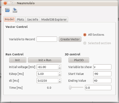
Figure 1. Neuronvisio Controls main interface. From this interface it is possible to initialize and launch simulations, or to start the 3D viewer. The “Model” tab allows simulation duration (tstop), numerical integration interval (dt), and resting potential values (mV) to be assigned.

It is now possible to create a new model, interactively using the console, or to load pre-existing one using a script. The suggested manner in which to load a pre-existing model written in Python is to integrate Neuronvisio into the main model script, inserting the two lines (number 12 and 13) as shown in the listing 1.

Listing 1: Medium Model example with Neuronvisio integration

"""
Cell model taken from the paper:
NEURON and Python
Hines et al.
Frontiers in Neuroinformatics
(2009)
DOI 10.3389/neuro.11/001.2009
"""

from itertools import chain

# Importing Neuronvisio
from neuronvisio.controls import Controls
controls = Controls()

# Importing the hoc interpreter
from neuron import h

# topology
soma = h.Section(name=’soma’)
apical = h.Section(name=’apical’)
basilar = h.Section(name=’basilar’)
axon = h.Section(name=’axon’)

apical.connect(soma, 1, 0)
basilar.connect(soma, 0, 0)
axon.connect(soma, 0, 0)

# geometry
soma.L = 30
soma.nseg = 1
soma.diam = 30

apical.L = 600
apical.nseg = 23
apical.diam = 1

basilar.L = 200
basilar.nseg = 5
basilar.diam = 2

axon.L = 1000
axon.nseg = 37
axon.diam = 1

# biophysics
for sec in h.allsec():
     sec.Ra = 100
     sec.cm = 1

soma.insert(’hh’)
apical.insert(’pas’)
axon.insert(’hh’)
basilar.insert(’pas’)

for seg in chain (apical, basilar):
   seg.pas.g = 0.0002
   seg.pas.e = -65

# ––––––––––- Instrumentation
 ––––––––––-
# synaptic input
syn = h.AlphaSynapse(0.5, sec=soma)
syn.onset = 0.5
syn.gmax = 0.05
syn.e = 0

3.2. Loading a Model from ModelDB

ModelDB (Hines et al., 2004) is a lightly curated repository of computational models, published in literature. While ModelDB accepts models in a variety of formats, those in NEURON format comprise a significant proportion, above 300 to date.

Neuronvisio incorporates the facility to quickly browse and load the models stored in ModelDB.

A listing of all NEURON models available on ModelDB is available in XML format, recording model characteristics and properties. An updated list is released with every new version of Neuronvisio. Between releases, it can be automatically updated by the user, through a script provided with the Neuronvisio source code. The XML file is parsed at run time and the content is loaded in a Qt tree widget, available in the ModelDB explorer tab, as shown in Figure 2. It is possible to browse models by year of publication, author, title, or a unique id number. Additionally, columns can be ordered alphabetically, and to assist in model selection, a keywords-based search is also provided.

FIGURE 2

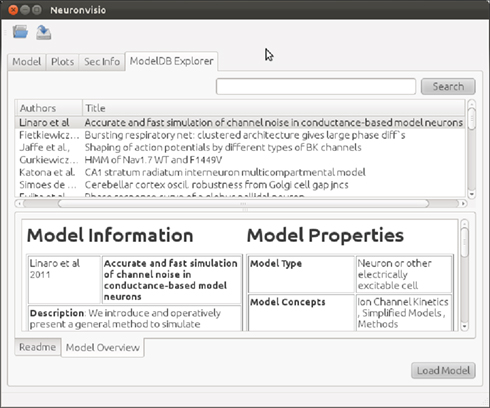
Figure 2. ModelDB Explorer tab. The ModelDB Explorer tab retrieves the list of NEURON models available in ModelDB. The two tabs in the lower panel provide a “Model Overview” and “README” information. Models can be selected in this panel. The Load Model button downloads, extracts, and compiles the selected model, loading it into the current session.

Each model entry presents two main information tabs: the Model Overview and the Readme tab. The former presents a summary of model characteristics, including information such as enumeration of channels by type (e.g., Calcium vs. Potassium), specifying cell type (e.g., medium spiny neuron vs. pyramidal neuron), the brain region, abstract of the paper. The README tab provides the README file associated with the model, if available, where the authors usually describe the model and how to perform simulations.

Any of the models selected on the ModelDB explorer tab can be loaded in Neuronvisio using the Load button. The software will fetch it from the web, extract, and compile the model’s files, and then launch it in the current session, allowing the user the possibility to explore and simulate it.

3.3. Simulating a Model with Neuronvisio

Most of the NEURON models available on ModelDB are written using the Hoc language, the legacy scripting language used before Python integration into NEURON. In the following section, we explain how to load models written in Hoc into Neuronvisio, using the pyramidal neuron from Mainen et al. (1995), id 8210 in ModelDB. This example model is distributed with Neuronvisio source code.

To use Neuronvisio with a hoc model, it is sufficient to import the module controls as for python, and then load the hoc model.

from neuronvisio.controls import Controls
from neuron import h
controls = Controls()
controls.load(’path/to/my_model.hoc’)

The simulation can be launched using the main Neuronvisio window (Figure 1), where it is possible to set the duration of the simulation (time stop), change the increment for the numerical integration (dt), and decide which resting membrane voltage should be used during the simulation. Due to the threaded implementation, Neuronvisio can be used simultaneously with the neuron.gui module.

To plot the simulation results, it is necessary to record at least one variable, usually the voltage, creating a HocVector (the data structure which NEURON uses to store the computed values of the variable). By default, Neuronvisio records the chosen variable in all the sections of the multicompartment model. It is possible to record the variable only from a specific section, by identifying it from the 3D representation and choosing Selected section. The vectors can be created entering the name of the variable, e.g., v for voltage, in the Variable to Record and click on Create Vector. One can launch the simulation clicking Init + Run on the “Model” tab, Figure 1.

3.4. Plotting and Saving a Simple Model

The recorded vectors are visible in the “Plot” tab, where the user can decide to plot any recorded variable within any section. Existing figures can be modified to include new points or lines, or new figures can be created. The Neuronvisio Qt4 main thread is integrated with the Qt matplotlib back-end, allowing interactive user-directed figure customization with the standard matplotlib commands. Figure 3 shows how to use to plot the vectors.

FIGURE 3

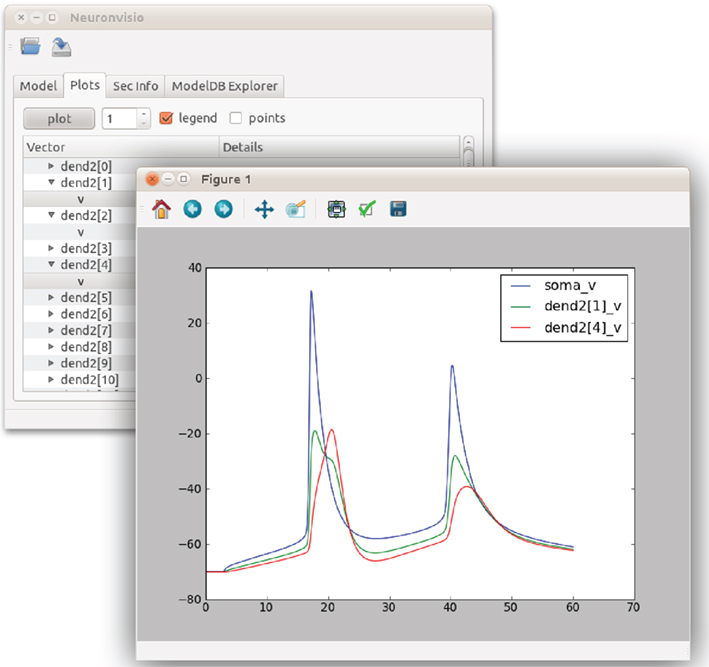
Figure 3. Matplotlib integration in Neuronvisio. The graph shows the time courses of the depolarization of the pyramidal Neuron, using the model from Mainen et al. (1995). The voltage of soma is plotted in blue, while two dendrites are plotted in red and green. The voltage (y-axis) is in millivolts and the time (x-axis) is in milliseconds.

3.5. 3D Representation and Animation Widow

Interactive 3D representations available through Neuronvisio allow full rotation and zoom for any NEURON model. A point-and-click selection allows inspection of section properties such as geometrical dimensions and biophysical properties.

To illustrate the 3D capabilities of Neuronvisio, we stimulate the example model injecting a current, using an IClamp mechanism, at time 3 ms in the soma, with a duration of 40 ms, and an amplitude of 0.25 nA.

Listing 2: Main file to load the pyramidal neurons

# Importing the NeuronVisio
from neuronvisio.controls import Controls
controls = Controls()
from neuron import h

# Load the script
h.load_file("demo.hoc")
## Insert an IClamp
st = h.IClamp(0.5, sec=h.soma)
st.amp = 0.25
st.delay = 3
st.dur = 40

The 3D representation can be used to investigate the evolution of any of the variables of the model. Figure 4 shows the depolarization of the pyramidal neuron. Using the time-slider in the “Model” tab under the “3D control” (Figure 1), it is possible to follow the depolarization of the sections through time. In this case the depolarization is initiated in the soma, and it is transmitted toward the dendrites.

FIGURE 4

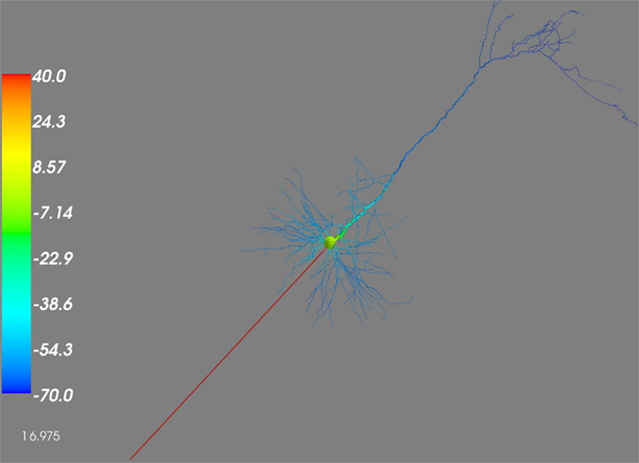
Figure 4. 3D rendering of the depolarization through the Pyramidal Neuron. The figure illustrates the depolarization state of the pyramidal neuron, at time 16.975 ms. The depolarization is initiated at the soma (yellow at +20 mV), and transmitted toward the dendrites (blue at −70 mv). The left color scale ranges from −70 mV (blue) through to +40 mV (red).

3.6. Saving User Customized Vectors

Numerical results of complex simulations are invaluable since: (i) their computational cost is expensive, requiring a lot of CPU/time and RAM, (ii) they deliver rich datasets, which can be analyzed in numerous ways, with most analysis being result-driven.

To record and analyze large models and complex simulations, the HocVector data structure intrinsic to NEURON may be not as flexible as required. The modeler may need a dedicated data structure to record several variables of interest, each of which are unique to a specific simulation. For example, in multiscale modeling, NEURON variables may be required to take as input the variables that are the output from a biochemical model. To track the interactions betweens the two parallel modeling systems, dedicated variables need to be created using a general python data structure. This is necessary because the variables are not computed in NEURON internally, therefore cannot be tracked by the classic vector object.

Another example comprises neuronal network simulations, where dedicated custom variable could follow a subset of the entire network, or any other variable which is not directly computed by NEURON.

For these reasons, a modular structure compliant with the Hierarchical Data Format (HDF; version 5), is used to store the simulation results. The HDF format was developed by an international consortium (The HDF Group, 2010) and provides the ability to store large amount of data in array form. A schema-free type is used to allocate the data, where the only requirement is to organize the data in a tree structure, consisting of nodes and leaves.

The main advantage of using HDF is that it allows indexed access of data. This permits the loading of large files, but retrieves only the specific nodes of the tree required by the Operating System. Therefore simulation results obtained from supercomputers or cluster computation can be reloaded using a lower specification computers, with a standard capacity RAM. This allows models of Terabyte dimensions to be launched on personal computers.

The organization of the storage file in Neuronvisio is shown in Figure 5. The data tree comprises two branches; the geometry branch (/geometry) stores the NeuroML representation of the morphology of the model, the results branch (/results) stores computed arrays of the simulations. The HocVectors are saved in the VecRef structure. The GenericRef node acts as placeholder for data structure customization, highlighting the extensibility of the design. The BaseRef class can be used to store any custom arrays not expressed as NEURON HocVectors. Every BaseRef object is contained in a group, which is specified by the group_id attribute. This attribute is automatically set to the name of the class, MyRef in this example. It is used in the selection interface presented to the user to assign the independent variable against which computed values should be plotted.

FIGURE 5

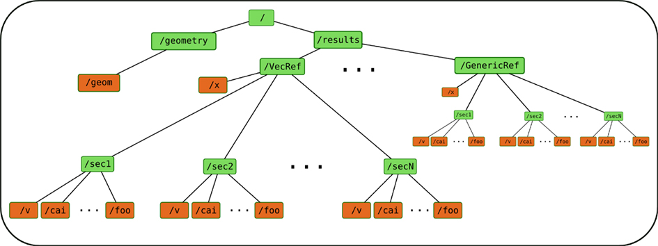
Figure 5. Structure of the HDF5 file used to store the computational results of a simulation. The data tree is composed of two branches: the geometry branch stores the NeuroML representation, the results branch stores computed arrays resulting from the simulations.

To subclass BaseRef, a class must be created, as shown 3:

Listing 3: Subclassing BaseRef into a custom myRef class

from neuronvisio.manager import BaseRef

class MyRef(BaseRef):
  def __init__(self, sec_name=None,
 vecs=None, detail=None):
      BaseRef.__init__(self)
      self.sec_name = sec_name
      self.vecs = vecs
      self.detail = detail

The class can then be used to create several myRef objects which will contain the section name, a dictionary, vecs; variables names act as a key and the value could either be a python list, a Numpy array, or an HocVector.

Listing 4: Creating a myRef object to save custom vectors

myRef = MyRef(sec_name=sec_name,
        vecs=vecs,
        detail=detail)

Every new myRef has to be added to the manager object, using the manager.add_ref method which takes two arguments: the myRef object and the x variable. (X is the independent variable, usually the time). If a custom time vector is not required, and the result-array has the length of the NEURON time, this can be retrieved using manager.groups[’t’].

Listing 5 shows how to import the Manager class, add the new sub-classed MyRef and save it.

Listing 5: Subclass BaseRef in myRef, creating vectors to record voltage and a custom dictionary vecs to record custom arrays, append them to the manager object and save the simulation results.

from neuronvisio.manager import Manager,
 BaseRef

# Subclassing BaseRef
class MyRef(BaseRef):
  def __init__(self, sec_name=None,
 vecs=None, detail=None):

      BaseRef.__init__(self)
      self.sec_name = sec_name
      self.vecs = vecs
      self.detail = detail

# Your model here
# ….

# Creating manager obj and vectors
 for the voltage
manager = Manager()
manager.add_all_vecRef(’v’) # Recording the
 voltage in each section

# Adding custom array, organized in a
 vecs dictionary
vecs = {’var1’ : numpy_array_var1,
       ’var2’ : numpy_array_var2}

myRef = MyRef(sec_name=sec_name,
       vecs=vecs)

# x is the independent variable, usually
 time
manager.add_ref(myRef, x)
# Logic to run the simulation
# ….

# Saving the vectors
filename = ’storage.h5’
manager.save_to_hdf(filename)

3.7. Reloading Stored Simulation Results

Large simulations are often run as batch jobs on computing clusters, with resulting data saved and analyzed at a later stage. It is possible to use this approach in Neuronvisio with the two methods of the controls class: save_to_hdf(filename), to save the results, and load_from_hdf(filename), to re-load them. The geometry of the neuron will be re-instantiated in NEURON and the simulation results will be re-mapped to the Neuronvisio data structure. It is be then possible to analyze the evolution of variables using the 3D viewer and to plot them directly from the Neuronvisio GUI, as if the simulation has just been performed.

4. Discussion

Developing complex multicompartment models is a difficult task which poses several problems, ranging from the description of the same differential equation for each section, to the handling of the cable equation optimization. Simulators such as NEURON and GENESIS can be used to create and run complex models in a more robust and simple manner. Around such simulators, an ecosystem of other complimentary software has been developed. One example is neuroConstruct (Gleeson et al., 2007), a software tool which can be used to create networks of multicompartment neurons and allows export to NEURON, GENESIS, and NeuroML. Another example is PyNN (Davison et al., 2008), which offers a standardized approach to the creation of networks of artificial neurons, which are to be run on several simulators, including NEURON. NeuroConstruct is written in Java and cannot interact directly with the NEURON kernel in real time, consequently models must be exported and then run in NEURON. PyNN is focused on the network level and cannot be currently used for multicompartment models.

We developed Neuronvisio to be highly integrated with NEURON and to solve three additional issues that arise when dealing with complex simulations: model visualization, automatic creation and plotting of vectors, and the storage of long running simulation results. These are not addressed satisfactorily by existing software. To facilitate download and launch a new model, we have integrated Neuronvisio, allowing one to download and load a model with a single click. Thus, Neuronvisio can be used as a tool to quickly interact with complex models, and may be suitable as a learning tool in computational neuroscience education.

The integration with ModelDB is modular by design, and in the future other databases able to export their models in NEURON compatible format, such as DOCQS (Sivakumaran et al., 2003) or Neuromorpho (Halavi et al., 2008), could also be incorporated.

When developing complex geometrical models, a quick, and accurate visualization is essential. The Neuronvisio 3D visualization and “Info” tab have been designed for this purpose. The existing “Model View” in NEURON displays a 2D model and list its global properties. The improved 3D visualization offered by Neuronvisio allows an interactive view, where the model can be rotated and enlarged. It is also possible to select a section, and examine it geometric and biophysical properties.

To simplify the process of launching a simulation and recording results, the instantiation of the HocVectors was automated, tracking all the variables in all sections of the model. User selection of variables to be tracked can be customized using the Neuronvisio manager API. The vectors can then be plotted using the integrated matplotlib plotting library and easily retrieved from the manager object for further analysis.

Complex models and simulations require the development of ad hoc solutions. These should not however compromised a clean design to store results. Neuronvisio stores results using the HDF standard in a custom modular file, which can incorporate user-specified arrays of any size. This file can then be reloaded, to recreate the same model structure, allowing one to analyze, plot, and explore the results in 3D space.

Conflict of Interest Statement

The authors declare that the research was conducted in the absence of any commercial or financial relationships that could be construed as a potential conflict of interest.

Acknowledgments

The authors would like to thank Gael Varoquaux for the help with the Mayavi library, Michael Hines, and Ted Carnevale for the timely answers on the NEURON forum and Nick Juty for extensively proofreading the manuscript.

Footnotes

1. ^http://www.riverbankcomputing.co.uk/software/pyqt/download
2. ^http://ipython.org
3. ^http://code.enthought.com/projects/mayavi/
4. ^http://matplotlib.sourceforge.net/
5. ^http://pypi.python.org/pypi/setuptools
6. ^http://www.pytables.org/

References

Bower, J., and Beeman, D. (1998). The Book of GENESIS: Exploring Realistic Neural Models with the General Neural Simulation System. New York: Springer-Verlag.

Carnevale, N. T., and Hines, M. L. (2006). The NEURON Book. Cambridge: Cambridge University Press.

Davison, A., Brüderle, D., Eppler, J., Kremkow, J., Muller, E., Pecevski, D., Perrinet, L., and Yger, P. (2008). PyNN: a common interface for neuronal network simulators. Front. Neuroinform. 2:11.

CrossRef Full Text

Dubois, P. F. (2007). Guest editor’s introduction: python: batteries included. Comput. Sci. Eng. 9, 7–9.

CrossRef Full Text

Ermentrout, B., and Mahajan, A. (2003). Simulating, analyzing, and animating dynamical systems: a guide to XPPAUT for researchers and students. Appl. Mech. Rev. 56, B53.

CrossRef Full Text

Gewaltig, M., and Diesmann, M. (2007). NEST (neural simulation tool). Scholarpedia J. 2, 1430.

CrossRef Full Text

Gleeson, P., Steuber, V., and Silver, R. (2007). Neuroconstruct: a tool for modeling networks of neurons in 3D space. Neuron 54, 219–235.

Pubmed Abstract | Pubmed Full Text | CrossRef Full Text

Goodman, D., and Brette, R. (2009). The brain simulator. Front. Neurosci. 3:2.

CrossRef Full Text

Halavi, M., Polavaram, S., Donohue, D., Hamilton, G., Hoyt, J., Smith, K., and Ascoli, G. (2008). NeuroMorpho.Org implementation of digital neuroscience: dense coverage and integration with the NIF. Neuroinformatics 6, 241–252.

Pubmed Abstract | Pubmed Full Text | CrossRef Full Text

Hines, M., Davison, A., and Muller, E. (2009). NEURON and python. Front. Neuroinform. 3:1.

CrossRef Full Text

Hines, M., Morse, T., Migliore, M., Carnevale, N., and Shepherd, G. (2004). ModelDB: a database to support computational neuroscience. J. Comput. Neurosci. 17, 7–11.

Pubmed Abstract | Pubmed Full Text | CrossRef Full Text

Hunter, J. D. (2007). Matplotlib: a 2D graphics environment. Comput. Sci. Eng. 9, 90–95.

CrossRef Full Text

Izhikevich, E. (2003). Simple model of spiking neurons. IEEE Trans. Neural Netw. 14, 1569–1572.

Pubmed Abstract | Pubmed Full Text | CrossRef Full Text

Lapicque, L. (1907). Recherches quantitatives sur l’excitation électrique des nerfs traitée comme une polarisation. J. Physiol. Pathol. Gen. 9, 620–635.

Mainen, Z., Joerges, J., Huguenard, J., and Sejnowski, T. (1995). A model of spike initiation in neocortical pyramidal neurons. Neuron 15, 1427–1439.

Pubmed Abstract | Pubmed Full Text | CrossRef Full Text

Perez, F., and Granger, B. (2007). IPython: a system for interactive scientific computing. Comput. Sci. Eng. 9, 21–29.

CrossRef Full Text

Ray, S., and Bhalla, U. (2008). PyMOOSE: interoperable scripting in python for MOOSE. Front. Neuroinform. 2:6.

Pubmed Abstract | Pubmed Full Text | CrossRef Full Text

Sivakumaran, S., Hariharaputran, S., Mishra, J., and Bhalla, U. (2003). The database of quantitative cellular signaling: management and analysis of chemical kinetic models of signaling networks. Bioinformatics 19, 408–415.

Pubmed Abstract | Pubmed Full Text | CrossRef Full Text

The HDF Group. (2010). Hierarchical Data Format Version 5, 2000-2010. Available at: http://www.hdfgroup.org/HDF5

Varoquaux, G., Vaught, T., and Millman, J. (eds). (2008). “Mayavi: Making 3D Data Visualization Reusable,” in Proceedings of the 7th Python in Science Conference, Pasadena, 51–56.