Memory-Efficient Analysis of Dense Functional Connectomes

1. Introduction

Graph-based analysis of dense connectomes allows for spatially precise mapping of fMRI-based functional connectivity patterns but is associated with considerable computational demands (van den Heuvel et al., 2008; Hayasaka and Laurienti, 2010; de Reus and Van den Heuvel, 2013; Fornito et al., 2013). As a result, some previous studies have been conducted at reduced spatial resolution (Buckner et al., 2009; Valencia et al., 2009; Zuo et al., 2012). However, most previous studies have not used dense connectomes at all, neither at the full nor at a reduced resolution. Instead, relatively coarse parcellations (or multiple regions of interests) were used to define network nodes (e.g., Salvador et al., 2005; Achard et al., 2006; Supekar et al., 2008; Fair et al., 2009; He et al., 2009; Supekar et al., 2009; Dosenbach et al., 2010; Fornito et al., 2011; Schoonheim et al., 2012; Agosta et al., 2013; Brier et al., 2014; Suo et al., 2015; Rocca et al., 2016). While the analysis of such parcellated connectomes offers many advantages and led to impactful findings, their spatial sensitivity is rather limited, as the use of region-level nodes typically involves the aggregation of fMRI time series from the incorporated voxels, at the cost of more detailed spatial information (Wang et al., 2010; Scheinost et al., 2012; Stanley et al., 2013). Such analyes are thus highly dependent on parcellation quality because regional and functional boundaries need to be relatively consistent to obtain meaningful results (Smith et al., 2011, 2013; Zuo and Xing, 2014; Jiang et al., 2015; Jiang and Zuo, 2016). In this regard, the suitability of a given parcellation also depends on the application because functional boundaries may vary between individuals (Biswal et al., 2010; Kelly et al., 2012), in the context of different tasks (Lohmann et al., 2016; Mišić and Sporns, 2016), or in association with dysfunction and disease (Matthews and Hampshire, 2016).

Dense connectomes, in contrast to parcellated connectomes, are less prone to these problems because the parcellation inherent to the data is used to define graphical nodes, so that the mixing of multiple, potentially dissimilar signals is avoided. To make the analysis of dense connectomes more computationally efficient, some efforts have recently been directed toward acceleration, e.g., through parallel computing (based on multi-core CPUs (Tomasi and Volkow, 2011; Loewe et al., 2014), GPUs (Wang et al., 2013), Intel^® Xeon Phi™ coprocessors (Wang et al., 2015), specialized vector hardware (Minati et al., 2014), or CPU instruction set extensions (Loewe et al., 2014)), or alternative measures of internodal association (Loewe et al., 2014; Minati et al., 2014).

By focusing on time efficiency, however, memory- and storage-related aspects are sometimes overlooked. With high-resolution data, a single connectivity matrix can easily surpass the available main memory of most computers. For example, at an isometric resolution of 2 mm, about 200,000 gray matter voxels exist in MNI template space. Using 4 bytes per element, the corresponding voxel-level connectivity matrix, or dense connectome (Van Essen and Ugurbil, 2012), would thus require about 149 GiB. Of course, there are some straightforward ways to reduce memory usage. As a side effect of the recently introduced grayordinate space, all gray matter can be represented by about 100,000 grayordinates because cortical data are modeled in surface space (Glasser et al., 2013), so that a grayordinate-based dense connectome would require only about 37.3 GiB. Due to matrix symmetry, it would further be sufficient to store only the upper or lower triangular part of a functional connectivity matrix, reducing memory occupancy by about 50%. Although the memory required to explicitly store connectivity matrices can be reduced in this way, they still remain too large for many applications, especially when considering high-resolution data or analyses across multiple subjects or conditions.

Here, we propose an object-based matrix representation that achieves a very low memory footprint by computing matrix elements on demand instead of explicitly storing them. In doing so, the memory required for a dense connectome reduces to the amount needed to store the underlying time series data. Even for data that exhibit a very high temporal resolution, this approach allows for immense reductions in memory requirements.

2. Materials and Methods

In the literature on functional connectivity, the terms matrix, graph, and connectome are often used somewhat interchangeably so that the exact meaning is often dependent on the context. Typically, based on a set of separate brain sites defined as nodes, pairwise statistical associations between the nodes' corresponding time series are used to derive a functional connectivity matrix. From a graph-theoretical perspective, this matrix can also be regarded as an undirected weighted graph or network, which is often binarized based on a connectivity threshold. Formally, an undirected binary graph G_B consists of two sets, a set of nodes and a set of pairwise internodal connections, or edges. G_B can be represented as an adjacency matrix B, where b_ij = 1 indicates that an edge exists between the two nodes i and j. The term connectome, originally defined in terms of structural brain connectivity (Sporns et al., 2005; Sporns, 2011), is now commonly used in a more ambiguous fashion often referring to brain connectivity graphs or networks of any kind (e.g., binary or weighted graphs, derived from structural, functional, or effective connectivity) and on multiple scales (e.g., microscopic, macroscopic, or at the systems level).

In the context of MRI, one can further distinguish between dense, i.e., voxel- or grayordinate-based, and parcellated connectomes (see e.g., Akil et al., 2011; Marcus et al., 2011; Glasser et al., 2013). In the latter, nodes are not individual voxels or grayordinates, but rather parcels, each of which typically comprises many voxels or grayordinates. Note that in this context dense connectomes could also be viewed as parcellated connectomes with atomic parcels. Note also that the use of the term “dense” here is distinct from its typical use to denote “dense” matrices as opposed to “sparse” matrices, even though a dense connectome can be represented by a dense connectivity matrix.

In this article, we describe our work with dense connectomes in mind. Of course, the proposed methods could be applied to parcellated connectomes as well, but, due to a much smaller number of nodes, such analyses are typically less challenging regarding computational efficiency.

The remainder of this section consists of three parts. We begin with a discussion of possible implementation variants for an object-based matrix representation, focusing on memory requirements and computation time. Next, programs for an example application (degree computation starting out from nodal time series data) based on the proposed matrix object implementation variants are described. The last part deals with the comparison of these programs with each other and with four additional programs based on external tools to assess the computational performance of the different implementation variants with respect to both time and memory efficiency.

2.1. Matrix Representation

Essentially, to design an object-based representation of a functional connectivity matrix (dense connectome), only three methods are required for interfacing with the object: a constructor (to create an object), an accessor (to access matrix elements), and a destructor (to free the resources acquired by the object during its lifetime when the object is destroyed). Let us consider the expected memory requirements and computation time of three storage schemes for such an object, which we will refer to as full-stored, half-stored, and on-demand.

2.1.1. Memory Requirements

In the full-stored scheme, upon object construction all pairwise internodal connectivity values are precomputed based on the nodes' corresponding time series data and the full connectivity matrix is stored in main memory. This requires memory in the order of N² + NT, where N is the number of nodes and T is the number of points in time for storing the full matrix and the time series data.

In the half-stored scheme, taking advantage of matrix symmetry, only the upper (or lower) triangular elements of the matrix are stored in order to save memory. This requires memory in the order of N(N − 1)/2 + NT.

In the on-demand scheme, a matrix element is computed on demand, i.e., once that specific element is accessed. This requires memory in the order of NT (the amount of memory needed for the underlying time series data).

Note that in the full- and half-stored schemes the time series data are needed during object construction only. After that, the memory required for the time series data could be deallocated if not otherwise needed. In contrast, in the on-demand scheme, the time series data need to be kept in memory until the object is destroyed. Nevertheless, because in the considered application domain N is much greater than T, the on-demand scheme provides superior memory efficiency compared to both other schemes.

2.1.2. Computation Time

To speed up execution, we consider (1) parallelization through concurrent computations on multiple CPU cores based on multi-threading, (2) data locality optimization (within each thread) through tiling, (3) vectorization through SIMD¹ instruction set extensions (within each thread), (4) using the tetrachoric correlation coefficient r_t instead of Pearson's r to estimate functional connectivity (the latter being used by the majority of previous studies).

2.1.2.1. Multi-threading

To benefit from parallelization by dividing the computations across multiple cores, parallelization through multi-threading (based on Pthreads) is employed in the half-stored scheme so that each of k threads computes (approximately) E/k matrix elements, where E = N(N − 1)/2 is the total number of matrix elements. For the on-demand scheme, parallelization through multi-threading cannot be implemented by the object for obvious reasons. However, it can be implemented by the client or application code, i.e., the code that uses the object (at the cost of additional programming efforts).

2.1.2.2. Data locality optimization

To benefit from data locality, the order in which the matrix elements are computed can be determined in an attempt to minimize the number of cache misses. For the half-stored scheme, we adopted a cache-oblivious tiling (COBL) approach to achieve this (Frigo et al., 1999; Prokop, 1999). Implementation details can be found in Loewe et al. (2014). For the on-demand scheme, data locality optimization has not been attempted, since, on the part of the matrix object, information on the order of accesses is not available in advance. Note that such information is often available on the part of the application code, but inter-dependencies between application code and implementation details of the matrix object should be avoided because the object implementation could change in the future. However, we discuss a special case below (see Section 2.1.3).

2.1.2.3. Vectorization

An fMRI data set can be represented by a data matrix ${\text{X}}^{N\times T}=(x_{ik})$, where 1 ≤ i ≤ N and 1 ≤ k ≤ T. By x_i = (x_i1, x_i2, ⋯, x_iT), i.e., the ith row of X, we denote the time series of the ith node. Using Pearson's r as a connectivity measure, the sample correlation matrix is given by ${\mathbf{\text{R}}}^{N\times N}=(r_{ij})$, where each matrix element can be computed as the mean of the products of the standard scores using

$r_{ij}=\frac{1}{T-1}{\displaystyle \sum _{k=1}^T}\left(\frac{x_{ik}-{\overline{x}}_i}{s_{x_i}}\right)\left(\frac{x_{jk}-{\overline{x}}_j}{s_{x_j}}\right)=\frac{z_i·z_j}{T-1},$

where ${\overline{x}}_i$, s_xi, and z_i (with z_i = (z_i1, z_i2, …, z_iT) and $z=\frac{x-\overline{x}}{s_x}$) are the sample mean, the corrected sample standard deviation, and the vector of standard scores corresponding to x_i, respectively. This equation can be rearranged to

$r_{ij}={\displaystyle \sum _{k=1}^T}\left(\frac{x_{ik}-{\overline{x}}_i}{\sqrt{(T-1)s_{x_i}^2}}\right)\left(\frac{x_{jk}-{\overline{x}}_j}{\sqrt{(T-1)s_{x_j}^2}}\right)=z_i^{\prime }·z_j^{\prime },$

where $s_{x_i}^2$ is the unbiased sample variance of x_i and $z_i^{\prime }$ is given by $z_i^{\prime }=(z_{i1}^{\prime },z_{i2}^{\prime },\dots ,z_{iT}^{\prime })$ with

$z_{ik}^{\prime }=\frac{x_{ik}-{\overline{x}}_i}{\sqrt{(T-1)s_{x_i}^2}}=\frac{x_{ik}-{\overline{x}}_i}{\sqrt{\sum _{l=1}^T{(x_{il}-{\overline{x}}_i)}^2}}.$

To compute R (formed by all pairwise correlation coefficients), we first compute $z_i^{\prime }$ for every node (pre-normalization; linear complexity) before computing $r_{i,j}=z_i^{\prime }·z_j^{\prime }$ for every node pair (quadratic complexity), which saves one division per pair compared to computing z_i and $\frac{z_i·z_j}{T-1}$, respectively.

Depending on the processor's capabilities, AVX or SSE2 instructions are used for SIMD-based vectorization. SIMD instructions allow for data-level parallelism by carrying out the same operation on multiple data elements simultaneously, using 256-bit (AVX) or 128-bit (SSE2) wide SIMD registers. For implementation details see Loewe et al. (2014).

2.1.2.4. Tetrachoric correlation estimation

Based on two binary variables x_b and y_b, the tetrachoric correlation coefficient r_t (Pearson, 1900) estimates the correlation of the two latent continuous-valued variables x_c and y_c, which are assumed to underlie x_b and y_b. Originally, r_t has been devised for those cases in which x_b and y_b are observable while x_c and y_c are not. As recently proposed, it can also be used as a computationally efficient, although less accurate, alternative to Pearson's r as a functional connectivity estimate (Loewe et al., 2014). The use of r_t for this purpose requires data reduction in the temporal domain: each nodal time series is initially binarized based on its median (Loewe et al., 2013, 2014). Assuming bivariate normality, the correlation between two original (real-valued) time series can then be estimated very efficently based on the binarized time series by the tetrachoric correlation coefficient, exploiting SSE2 and the POPCNT instruction for SIMD-based vectorization for the necessary computations. If these instructions are not supported by the processor, an alternative, albeit less efficient, implementation based on a 16-bit lookup table can be used instead. For implementation details see Loewe et al. (2014). An additional advantage is that a binarized time series, being stored in the bits of integer variables, requires only a fraction of the memory that the original time series requires. This compression seems to render data locality optimization unnecessary for most data sets, presumably because the entire binarized time series data set can be stored in the CPU cache.

Note that the considerations made above for the half-stored scheme are also valid for the full-stored scheme. However, we decided to forego an actual implementation of this scheme within our framework at this point since it exhibits the highest memory requirements and a full-stored matrix representation is easily achieved based on already available software (for example, Matlab's corrcoef).

2.1.3. Cache-Based Implementation

To accomodate situations where all matrix elements need to be traversed, but the order of traversal is essentially arbitrary, a cache-based storage scheme was additionally devised. In this scheme, upon construction, the matrix object is initialized such that a cache of user-specified size is maintained internally. While client code uses iterator functions to traverse the elements, the object internally fills its cache when necessary.

Since the order of traversal is determined by the object, both data locality (COBL) and multi-threading can be exploited when the cache is filled. Thus, similar to the half-stored scheme, data locality optimization and multi-threading can be implemented by the matrix object, which reduces the programmer's efforts when implementing applications, compared to the on-demand scheme. As mentioned above, for the on-demand scheme multi-threading has to be implemented by application code, and data locality optimization cannot be used at all, if inter-dependencies between matrix object implementation and client code are to be avoided. On the other hand, it is not possible to parallelize the traversal when using the cache-based variant, which could be a significant disadvantage in some situations.

2.2. Application: Degree Centrality

In this section, the task of node degree computation based on nodal time series data will serve as an example application to assess the performance of the different matrix object implementations with respect to both time and memory efficiency. The node degree, or degree centrality, is a simple graph-theoretical metric aimed at investigating the importance of individual nodes in a binary graph (Nieminen, 1974; Freeman, 1979). It is defined for each node as the number of other nodes to which it is connected. More formally, given a binary graph G_B, the degree k_i of a node i is defined as $k_i=\sum _j^{\left|N\right|}{b}_{i,j}$, where i, j ∈ N, i ≠ j, and N is the set of nodes. In the neuroimaging literature, centrality measures have been used as a means to identify and analyze network hubs in the human brain (Buckner et al., 2009; Lohmann et al., 2010; Tomasi and Volkow, 2010, 2012; Wink et al., 2012; Zuo et al., 2012; Di Martino et al., 2013; van den Heuvel and Sporns, 2013; Binnewijzend et al., 2014; Markett et al., 2014, 2016; Schaefer et al., 2014).

2.2.1. Programs

Combining the storage schemes half-stored, on-demand, and cache-based with the two functional connectivity estimates, Pearson's r and tetrachoric correlation coefficient r_t, we arrive at six matrix object configurations. We will denote these by FCMAT/s/$\widehat{\rho }$, where s indicates the storage scheme with s ∈ {half-stored, on-demand, cache-based}, and $\widehat{\rho }$ indicates the functional connectivity estimate² with $\widehat{\rho }\in \left\{r,r_t\right\}$.

For typical fMRI data sets, data locality optimization turned out not to be beneficial if r_t is used as the functional connectivity estimate. Only for a very large number of points in time is a benefit observed. Presumably, this is because the binarized time series, due to efficient bitwise storage, take up far less memory than the original time series, thus enabling efficient CPU cache usage without additional optimizations. This is why the cache-based variant is not combined with r_t here. For the same reasons, data locality optimization is used for FCMAT/half-stored/r, but not for FCMAT/half-stored/r_t.

The matrix object variants were implemented in C. The programs for degree computation based on the matrix object were also written in C, but Matlab integration is provided via MEX. A corresponding open source software package is available for download³. In addition, four programs for degree computation based on Matlab functions or Matlab-based third-party software have been created. These programs use corrcoef (Matlab built-in), corr (Matlab Statistics Toolbox), IPN_fastCorr, and IPN_calLCAM (from the Matlab toolbox “IPN_voxelGraph” by Xi-Nian Zuo available at Matlab File Exchange⁴) for matrix computation, respectively. Note that “IPN_voxelGraph” is now part of a new, much more extensive toolbox called “Connectome Computation System”⁵ (Xu et al., 2015).

In principle, each program first derives a weighted graph G (correlation matrix) from the data, then derives a binary graph G_B (adjacency matrix) from G based on a functional connectivity threshold, and finally determines the degree k_i of each node i in G_B. Note that these basic steps are not necessarily performed explicitly.

The programs based on corrcoef, corr, and IPN_fastCorr use a full-stored matrix representation as they first compute an N × N correlation matrix. This matrix is thresholded to derive a binary adjacency matrix. Then, degrees are obtained by summation over rows (or columns) of the adjacency matrix.

The programs using FCMAT/half-stored/* first create the matrix object, which, upon creation, computes and internally stores the upper triangle of the correlation matrix based on the input data. In doing so, multi-threading, data locality optimization, and vectorization are used. Data locality optimization is used only in combination with Pearson's r for the reasons stated above. The matrix elements are then traversed using the object's accessor method (traversal is parallelized using multiple threads). Upon access, the appropriate pre-computed element is returned by the matrix object. If an element exceeds the threshold, the degree of the corresponding nodes is incremented.

The programs using FCMAT/on-demand/* first create the matrix object, which, upon creation, pre-normalizes or binarizes the input data. The matrix elements are then traversed using the object's accessor method (traversal is parallelized using multiple threads). Upon access, the appropriate element is computed, and returned by the matrix object. If an element exceeds the threshold, the degree of the corresponding nodes is incremented. Neither the correlation matrix nor the adjacency matrix is explicitly stored.

The program using FCMAT/cache-based/r first creates the matrix object, which, upon creation, initializes the internal cache. The matrix elements are then traversed using the iterator functions. When the next matrix element is requested during traversal, the matrix object checks if the next element is in the cache and retrieves it from there, if that is the case. If not, the cache is filled by computing the next “tile of matrix elements” exploiting multi-threading, data locality optimization, and vectorization in the process. The matrix element along with its coordinates is then returned by the matrix object. Thresholding and incrementation of the appropriate degrees are conducted during traversal in the same way as for the other variants, with the notable exception that the traversal (and hence also thresholding and degree incrementation) is not parallelized.

The program using IPN_calLCAM does not follow any of the schemes described above. Based on a pre-defined correlation threshold, it employs a block-wise approach to construct a sparse adjacency matrix directly from the data (Zuo et al., 2012). The adjacency matrix is efficiently stored using Matlab's sparse matrix functionality. Explicit storage of the full correlation matrix is thus avoided, while memory requirements during adjacency matrix construction depend on the selected block size, and memory requirements for the final adjacency matrix depend on its sparsity. To efficiently compute the correlation values for each block, IPN_calLCAM internally uses IPN_fastCorr. Note that IPN_calLCAM is not applicable to analyses that use the (weighted) connectivity matrix rather than the adjacency matrix.

2.2.2. Benchmarks

Benchmarks were conducted using Matlab (R2011b) on two machines, a desktop computer with an Intel Core i7-3960X CPU (3.30 GHz, 6 cores, hyper-threading disabled) and 64 GB of main memory running Linux (openSUSE 13.1, Kernel 3.11), and a server with two Intel Xeon E5-2697 v2 CPUs (2.7 GHz, 12 cores, hyper-threading enabled) and 256 GB of main memory running Linux (Ubuntu 12.04.5 LTS, Kernel 3.13). The C/MEX routines that are part of the programs that use the matrix object were compiled using the GNU C compiler gcc (optimization level 3; version 4.8.1 and 4.6.3 on the desktop and the server system, respectively). To assess the memory usage of the programs, we used the function monMem⁶, which, in turn, uses the Linux proc file system to monitor Matlab's resident memory size during program execution.

Three input data sets with a different number of nodes (60,000, 120,000, and 240,000) and T = 256 points in time were generated using pseudo-random single-precision floating point numbers. Storage of the full matrix (assuming 4 byte per element) would require 13.4, 53.6, and 214.6 GiB of memory for 60,000, 120,000, and 240,000 nodes, respectively. The correlation threshold was chosen such that the density of the resulting binary graph was approximately 0.01. For IPN_calLCAM, we used 10 (for the data sets with 60,000 and 120,000 nodes) and 25 blocks (for the data set with 240,000 nodes). The number of threads was varied between 1 and 6 on the desktop computer and between 1 and 48 on the server. For the programs based on the FCMAT variants the number of threads was controlled via the corresponding parameter. For the programs based on corrcoef, corr, IPN_fastCorr, and IPN_calLCAM the number of threads was controlled using the Matlab function maxNumCompThreads.

3. Results

To assess the performance of the different FCMAT variants, we used the computation of node degrees based on nodal time series data as an example application. Experiments were conducted on the two machines described above. Note that, depending on the number of nodes of the input data set and the available main memory, some tests could not be conducted due to insufficient memory on the respective systems. In correspondence with the number of logical processors on each system, the number of threads was varied between 1 and 6 on the desktop computer and between 1 and 48 on the server.

In Figure 1, the main results regarding memory requirements and computation time are illustrated. Here, only the best result is reported for each program, i.e., the result based on the number of threads for which the elapsed time was shortest for that program. This seemed the most appropriate since some programs continually gained performance from additional threads, while for other programs additional threads turned out to be detrimental to their performance after a certain optimal number of threads was exceeded. The performance gained by each program through multi-threading and the cache effectiveness in terms of cache misses are illustrated in Figures 2 and 3, respectively.

FIGURE 1

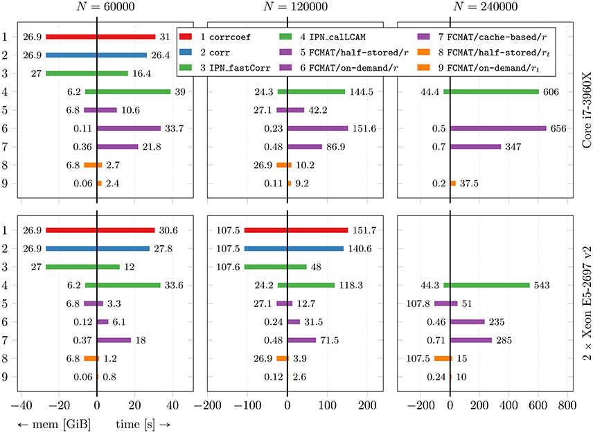
Figure 1. Performance comparison with respect to time and memory efficiency. The compared programs for degree computation are based on corrcoef (1), corr (2), IPN_fastCorr (3), IPN_calLCAM (4) and the proposed functional connectivity matrix object FCMAT using the half-stored (5 and 8), the on-demand (6 and 9) and the cache-based variant (7). The programs 1-7 use Pearson's r as a functional connectivity estimate; the programs 8 and 9 use the tetrachoric correlation coefficient r_t. Comparisons were conducted on two machines, a desktop computer with an Intel Core i7-3960X CPU and 64GB of main memory, and a server with two Intel Xeon E5-2697 v2 CPUs and 256GB of main memory. The number of threads was varied between 1 and 6 on the desktop computer and between 1 and 48 on the server. For each program, only the best result is reported, i.e., the result based on the number of threads for which the elapsed time was shortest for that program. See Figure 2 for more detailed results regarding the performance gained by each program through multi-threading. The reported results are averages from 10 runs. For details see text. The number of timepoints T was fixed at T = 256. N: number of nodes; mem [GiB]: peak memory in GiB; time [s]: elapsed time in seconds.

FIGURE 2

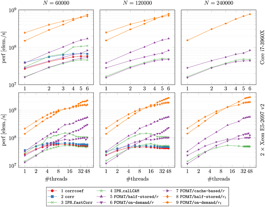
Figure 2. Performance gained through multi-threading. The compared programs for degree computation and the two machines on which the comparisons were conducted are the same as in Figure 1. The reported results are averages from 10 runs on each machine. The number of timepoints T was fixed at T = 256. N: number of nodes; perf [elem./s]: performance in number of computed elements per second.

FIGURE 3

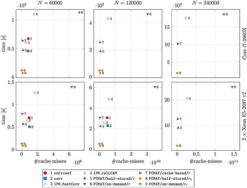
Figure 3. Speed vs. cache misses. The compared programs for degree computation and the two machines on which the comparisons were conducted are the same as in Figures 1 and 2. The reported results are averages from 10 runs on each machine. The number of timepoints T was fixed at T = 256. N: number of nodes; time [s]: elapsed time in seconds.

3.1. Memory Requirements and Maximum Performance

The benchmarks showed that the programs based on corrcoef (1), corr (2), and IPN_fastCorr (3) had the highest memory requirements of all programs (Figure 1), which was expected because they employ full matrix storage. However, they used more memory than expected (Table 1). More specifically, the peak memory of these three programs was about two times higher than expected. Instead of approximately 4(N² + NT) bytes it was about twice that much, for example, approximately 27 GiB instead of the expected 13.5 GiB for N = 60,000. Of these three programs, IPN_fastCorr executed fastest, sometimes up to 3× faster than corrcoef, while corr was only slightly faster than corrcoef (Figure 1).

TABLE 1

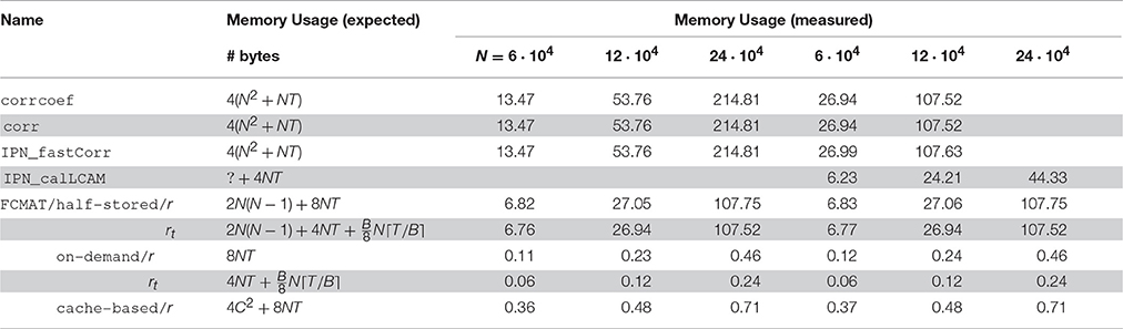
Table 1. Expected and measured memory usage.

The memory requirements of IPN_calLCAM (4) depend on the number of blocks S, so that it is possible to reach lower memory requirements at the cost of increased computation time (due to additional overhead) by choosing a greater number of blocks. Using S = 10, S = 10, and S = 25, the program peaked at approximately 6.2, 24.3, and 44.4 GiB for N = 60,000, N = 120,000, and N = 240,000, respectively. For N = 60,000, IPN_calLCAM executed about 10–30% slower than corrcoef (depending on the system), while it was about 20% faster for N = 120,000 on the server (Figure 1).

The programs based on FCMAT/half-stored/r (5) and FCMAT/half-stored/r_t (8) showed the expected memory requirements, which were significantly reduced compared to the programs based on full storage, but still very high. They peaked at about about 7, 27, and 108 GiB for N = 60,000, N = 120,000, and N = 240,000, respectively. Here, the expected memory requirements were computed as

$\underset{\text{resulting matrix}}{\underbrace{2N(N-1)}}+\underset{\text{original data}}{\underbrace{4NT}}+\underset{\text{normalized data}}{\underbrace{4NT}} \text{bytes}$

for FCMAT/half-stored/r, and

$\underset{\text{resulting matrix}}{\underbrace{2N(N-1)}}+\underset{\text{original data}}{\underbrace{4NT}}+\underset{\text{binarized data}}{\underbrace{\frac{B}{8}N\lceil T/B\rceil }} \text{bytes}$

where B is the number of bits per integer variable, for FCMAT/half-stored/r_t (Table 1). Depending on the system and the number of nodes, FCMAT/half-stored/r and FCMAT/half-stored/r_t ran between 3 and 12× and 11 and 39× faster than corrcoef (Figure 1).

The memory requirements of the programs based on FCMAT/on-demand/r (6) and FCMAT/on-demand/r_t (9) remained below 0.5 GiB for all three data sets. Specifically, the former peaked at approximately 0.12, 0.23, and 0.46 GiB corresponding to the expected 4NT (original data) + 4NT (normalized data) bytes, while the latter peaked at approximately 0.06, 0.12, and 0.24 GiB, corresponding to 4NT (original data) + $\frac{B}{8}N\lceil T/B\rceil$ (binarized data) bytes, for N = 60,000, N = 120,000, and N = 240,000, respectively. Depending on the system and the number of nodes, FCMAT/on-demand/r executed 1.8–3.6× slower than the corresponding half-stored variant FCMAT/half-stored/r, while FCMAT/on-demand/r_t executed up to 1.5× faster than its half-stored pendant FCMAT/half-stored/r_t (Figure 1).

The program based on FCMAT/cache-based/r (7) peaked at approximately 0.36 (N = 60,000), 0.48 (N = 120,000), and 0.71 GiB (N = 240,000) corresponding to the expected 4C² + 8NT bytes (using a cache tile size of C = 8192). On the desktop, depending on the number of nodes, FCMAT/cache-based/r executed about 1.6–1.9× faster than the corresponding on-demand variant and about 2.1× slower than the corresponding half-stored variant. On the server, depending on the number of nodes, it executed about 1.2–3× slower than the on-demand variant and about 5.5× slower than the half-stored variant (Figure 1).

3.2. Performance Gain through Multi-Threading

After reaching a performance maximum at a certain number of threads, the programs using corrcoef, corr, IPN_fastCorr, and IPN_calLCAM exhibited stagnating and even decreasing performance upon adding more computational threads (Figure 2, especially on the server). A similar observation can be made for FCMAT/cache-based/r, although performance seems to reach a plateau state of maximum performance, such that additional threads do not improve performance further but no performance decrease is observed either. On a related note, FCMAT/cache-based/r is significantly faster than FCMAT/on-demand/r for smaller numbers of threads, but this advantage is lost in the course of more threads being added (Figure 2, especially on the Xeon system). This is because FCMAT/on-demand/r sustains a relatively constant high performance gain per thread over the entire range of the number of threads. A similar observation can be made for FCMAT/on-demand/r_t and FCMAT/half-stored/r_t (Figure 2, both systems).

3.3. Cache Misses

To assess how well the attempted data locality optimization worked (especially with regard to FCMAT/cache-based/r), we compared the programs' computation time with the number of cache misses (Figure 3). Note that these measurements were conducted using only one thread.

Comparing the programs using FCMAT/*/r, the on-demand variant had the greatest number of cache misses and correspondingly exhibited the lowest performance (with respect to computation time). The other two variants exhibited a similar number of cache misses (both had significantly fewer cache misses than the on-demand variant), but the half-stored variant still ran faster than the cache-based variant, while both ran significantly faster than the on-demand variant. Similarly, the programs using corrcoef and corr exhibited a similar number of cache misses, but the latter outperformed the former. Furthermore, corrcoef was about as fast as FCMAT/cache-based/r and corr was about as fast as FCMAT/half-stored/r, although corrcoef and corr exhibited more cache misses than the other two. The program using IPN_fastCorr exhibited a lower number of cache misses than both corrcoef and corr but higher than FCMAT/half-stored/r and FCMAT/cache-based/r. Its performance ranked between that of corrcoef and corr. The number of cache misses for IPN_calLCAM was comparable with that of corrcoef and corr, but it was significantly slower than both.

4. Discussion

Dense connectomes allow for spatially more fine-grained connectivity analyses, but are associated with significant computational demands (van den Heuvel et al., 2008; Hayasaka and Laurienti, 2010; de Reus and Van den Heuvel, 2013; Fornito et al., 2013). Available computing resources are often insufficient to meet these demands, so that dense connectome analyses become infeasible (e.g., Smith et al., 2014). In an attempt to address this issue, we presented an object-based functional connectivity matrix representation (FCMAT) and corresponding implementation variants, tailored for the analysis of dense functional connectomes. Based on theoretical considerations and benchmarks, different implementation variants of this object and four additional programs (based on available Matlab functions and Matlab-based third-party software) were compared with regard to their computational efficiency in terms of both memory requirements and computation time.

The most memory-efficient FCMAT variant avoids explicit matrix storage by computing matrix elements on demand based on the underlying time series data (FCMAT/on-demand/*). Since, in the considered application domain, the number of nodes is much greater than the number of scans, the memory requirements of a dense connectome are effectively reduced by orders of magnitude compared to explicit storage of the connectivity matrix.

However, explicit storage has an advantage over on-demand computation when it comes to computation time because data locality optimization can be employed. Accordingly, the implementation using explicit matrix storage, FCMAT/half-stored/*, is the fastest of the presented variants. It is also faster than the alternatives based on explicit storage (full-stored), corrcoef (Matlab built-in), corr (Matlab Statistics Toolbox), and IPN_fastCorr (from the Matlab toolbox “IPN_voxelGraph” by Xi-Nian Zuo)⁷. Of these, IPN_fastCorr was significantly faster than the other two. Regarding memory requirements, FCMAT/half-stored/* has an advantage over the full-stored programs because it exploits matrix symmetry in order to save memory. Nevertheless, the memory requirements of FCMAT/half-stored/* are still too high for many applications.

In addition to FCMAT/half-stored/* and FCMAT/on-demand/*, a third, cache-based variant, FCMAT/cache-based/r, was implemented in an attempt to combine the advantages of the first two. Regarding time efficiency, this variant is at an advantage over the on-demand variant, in that it can use data locality optimization, which is reflected in the observed reduction in cache misses. It is, however, at a disadvantage compared to the half-stored variant, because of the overhead that results from maintaining the cache. Regarding memory efficiency, the cache-based scheme requires far less memory than the half-stored scheme although not quite as little as the on-demand scheme (assuming a sensible choice for the cache size). Depending on the application, the cache-based scheme may thus provide a reasonable compromise between explicit storage and on-demand computation, by being more memory-efficient than the former, but faster than the latter. However, while the computation of the matrix elements by the matrix object can be parallelized (during cache fills), the traversal of these elements by the client code can not be parallelized. If additional, potentially expensive, computations need to be conducted during matrix traversal, this drawback can tip the balance in favor of one of the other implementations for some applications (see Amdahl, 1967). In this context, the number of cores of the system also needs to be taken into account. As the benchmarks illustrate, the on-demand variant should be chosen over the cache-based variant on a system with many cores because the impact of this issue increases with the degree of parallelization.

Considering the example application used for benchmarking, each of the created programs for node degree computation (implicitly or explicitly) derives a binary adjacency matrix from the connectivity matrix based on a threshold. Depending on the thresholding scheme used (e.g., based on graph density), an additional run through the data may be necessary to determine the threshold in terms of absolute correlation before the degree map can be computed. For those programs that do not operate on the explicitly stored connectome (IPN_calLCAM, FCMAT/on-demand/* and FCMAT/cache-based/r), this entails that the correlation values need to be computed twice. This example makes clear that, especially in situations where the matrix or connectome will be used more than once (e.g., when subjected to multiple analyses), explicit storage should be used if it is affordable (with respect to the available main memory) in order to save computation time.

Although the present programs provide a highly efficient way of conducting analyses, there are some limitations that should be noted. First, in cases of extremely large multi-subject data sets (in terms of number of subjects or scans), too much memory may still be required for these methods to be applied because the time series data of all subjects could already be too large to be stored in main memory. In some cases, the analysis procedure could be adapted to hold only a sufficiently small partition of the data in memory at any given time. Second, the current implementation only supports Pearson's r and r_t. In the case of dense connectomes, the number of nodes and therefore edges is a lot higher than the number of scans, so that the underlying population correlation ρ cannot be estimated very accurately using r or r_t (e.g., Varoquaux and Craddock, 2013). The extension of FCMAT to support other, possibly better estimates is a subject for future work. Finally, while FCMAT provides the basis for the efficient analysis of dense connectomes, the tools for the analyses themselves (for example, graph-theoretical analyses or statistical inference), still need to be implemented (on top of it), which, depending on the analysis in question, may prove to be a lot more difficult.

To summarize, when considering the computational burden of dense functional connectome analysis, the manner in which connectivity matrices are represented plays an important role. We show here that a set of complementary implementation variants of an object-based matrix representation (FCMAT) provide a highly efficient foundation for dense connectome analysis. If affordable in terms of available memory, explicit matrix storage should be used, since it provides the best performance in terms of CPU time. However, if its memory requirements render the use of explicit storage infeasible, on-demand computation or cache-based iteration provide memory-efficient alternatives. In particular, the on-demand and cache-based implementation variants allow for the analysis of larger data sets on commonly available hardware, which may not have been possible before, based on explicit storage. With the ever-growing need for maximal spatial precision and resolution among large sets of subjects in fMRI connectivity analyses, the development of efficient tools such as these is paramount to the advancement of our understanding of the human brain.

Author Contributions

KL conceived of the study. KL and CB wrote the software. KL carried out the benchmarks. KL wrote the manuscript. SD, MS, RK, and CB edited the manuscript. All authors read and approved the final manuscript.

Funding

This work was in part supported by Deutsche Forschungsgemeinschaft SFB 779 (A14N).

Conflict of Interest Statement

The authors declare that the research was conducted in the absence of any commercial or financial relationships that could be construed as a potential conflict of interest.

Footnotes

1. ^A single instruction can be applied to multiple data in parallel using CPU instruction set extensions such as SSE2 (Streaming SIMD Extensions, version 2) or AVX (Avanced Vector eXtensions).

2. ^The symbol ρ was chosen because the functional connectivity estimates that are used here, r and r_t, are, in fact, correlation estimates (estimating a hypothetical population correlation ρ). This involves the simplistic assumption of time series stationarity (Hutchison et al., 2013; Zalesky et al., 2014) of the involved time series and also the assumption of bivariate normality between every two time series (Hlinka et al., 2011).

3. ^http://www.kristianloewe.com/software and https://github.com/kloewe/conan.

4. ^http://www.mathworks.com/matlabcentral/fileexchange/32553-ipn-voxelgraph.

5. ^https://github.com/zuoxinian/CCS.

6. ^https://github.com/kloewe/util-m.

7. ^http://www.mathworks.com/matlabcentral/fileexchange/32553-ipn-voxelgraph.

References

Achard, S., Salvador, R., Whitcher, B., Suckling, J., and Bullmore, E. (2006). A resilient, low-frequency, small-world human brain functional network with highly connected association cortical hubs. J. Neurosci. 26, 63–72. doi: 10.1523/JNEUROSCI.3874-05.2006

PubMed Abstract | CrossRef Full Text | Google Scholar

Agosta, F., Sala, S., Valsasina, P., Meani, A., Canu, E., Magnani, G., et al. (2013). Brain network connectivity assessed using graph theory in frontotemporal dementia. Neurology 81, 134–143. doi: 10.1212/WNL.0b013e31829a33f8

PubMed Abstract | CrossRef Full Text | Google Scholar

Akil, H., Martone, M., and Van Essen, D. (2011). Challenges and opportunities in mining neuroscience data. Science (New York, NY) 331:708. doi: 10.1126/science.1199305

PubMed Abstract | CrossRef Full Text | Google Scholar

Amdahl, G. M. (1967). “Validity of the single processor approach to achieving large scale computing capabilities,” in Proceedings of the April 18-20, 1967, Spring Joint Computer Conference (New York, NY: ACM), 483–485. doi: 10.1145/1465482.1465560. Available online at: http://dl.acm.org/citation.cfm?id=1465560

CrossRef Full Text

Binnewijzend, M. A., Adriaanse, S. M., Flier, W. M., Teunissen, C. E., Munck, J. C., Stam, C. J., et al. (2014). Brain network alterations in alzheimer's disease measured by eigenvector centrality in fmri are related to cognition and csf biomarkers. Hum. Brain Mapp. 35, 2383–2393. doi: 10.1002/hbm.22335

PubMed Abstract | CrossRef Full Text | Google Scholar

Biswal, B., Mennes, M., Zuo, X., Gohel, S., Kelly, C., Smith, S., et al. (2010). Toward discovery science of human brain function. Proc. Natl. Acad. Sci. U.S.A. 107:4734. doi: 10.1073/pnas.0911855107

PubMed Abstract | CrossRef Full Text | Google Scholar

Brier, M. R., Thomas, J. B., Fagan, A. M., Hassenstab, J., Holtzman, D. M., Benzinger, T. L., et al. (2014). Functional connectivity and graph theory in preclinical alzheimer's disease. Neurobiol. Aging 35, 757–768. doi: 10.1016/j.neurobiolaging.2013.10.081

PubMed Abstract | CrossRef Full Text | Google Scholar

Buckner, R., Sepulcre, J., Talukdar, T., Krienen, F., Liu, H., Hedden, T., et al. (2009). Cortical hubs revealed by intrinsic functional connectivity: mapping, assessment of stability, and relation to alzheimer's disease. J. Neurosci. 29, 1860–1873. doi: 10.1523/JNEUROSCI.5062-08.2009

PubMed Abstract | CrossRef Full Text

de Reus, M. A., and Van den Heuvel, M. P. (2013). The parcellation-based connectome: limitations and extensions. Neuroimage 80, 397–404. doi: 10.1016/j.neuroimage.2013.03.053

PubMed Abstract | CrossRef Full Text | Google Scholar

Di Martino, A., Zuo, X.-N., Kelly, C., Grzadzinski, R., Mennes, M., Schvarcz, A., et al. (2013). Shared and distinct intrinsic functional network centrality in autism and attention-deficit/hyperactivity disorder. Biol. Psychiatry 74, 623–632. doi: 10.1016/j.biopsych.2013.02.011

PubMed Abstract | CrossRef Full Text | Google Scholar

Dosenbach, N., Nardos, B., Cohen, A., Fair, D., Power, J., Church, J., et al. (2010). Prediction of individual brain maturity using fMRI. Science 329, 1358–1361. doi: 10.1126/science.1194144

PubMed Abstract | CrossRef Full Text | Google Scholar

Fair, D., Cohen, A., Power, J., Dosenbach, N., Church, J., Miezin, F., et al. (2009). Functional brain networks develop from a local to distributed organization. PLoS Comput. Biol. 5:e1000381. doi: 10.1371/journal.pcbi.1000381

PubMed Abstract | CrossRef Full Text | Google Scholar

Fornito, A., Yoon, J., Zalesky, A., Bullmore, E. T., and Carter, C. S. (2011). General and specific functional connectivity disturbances in first-episode schizophrenia during cognitive control performance. Biol. Psychiatry 70, 64–72. doi: 10.1016/j.biopsych.2011.02.019

PubMed Abstract | CrossRef Full Text | Google Scholar

Fornito, A., Zalesky, A., and Breakspear, M. (2013). Graph analysis of the human connectome: promise, progress, and pitfalls. Neuroimage 80, 426–444. doi: 10.1016/j.neuroimage.2013.04.087

PubMed Abstract | CrossRef Full Text | Google Scholar

Freeman, L. (1979). Centrality in social networks conceptual clarification. Soc. Netw. 1, 215–239. doi: 10.1016/0378-8733(78)90021-7

CrossRef Full Text | Google Scholar

Frigo, M., Leiserson, C., Prokop, H., and Ramachandran, S. (1999). “Cache-oblivious algorithms,” in Proceedings 40th IEEE Symposium on Foundations of Computer Science (FOCS'99, New York, NY) (Piscataway, NJ: IEEE Press), 285–297. doi: 10.1109/sffcs.1999.814600

CrossRef Full Text

Glasser, M. F., Sotiropoulos, S., Wilson, J., Coalson, T., Fischl, B., Andersson, J., et al. (2013). The minimal preprocessing pipelines for the human connectome project. Neuroimage 80, 105–124. doi: 10.1016/j.neuroimage.2013.04.127

PubMed Abstract | CrossRef Full Text | Google Scholar

Hayasaka, S., and Laurienti, P. (2010). Comparison of characteristics between region-and voxel-based network analyses in resting-state fMRI data. Neuroimage 50, 499–508. doi: 10.1016/j.neuroimage.2009.12.051

PubMed Abstract | CrossRef Full Text | Google Scholar

He, Y., Wang, J., Wang, L., Chen, Z. J., Yan, C., Yang, H., et al. (2009). Uncovering intrinsic modular organization of spontaneous brain activity in humans. PLoS ONE 4:e5226. doi: 10.1371/journal.pone.0005226

PubMed Abstract | CrossRef Full Text | Google Scholar

Hlinka, J., Palus, M., Vejmelka, M., Mantini, D., and Corbetta, M. (2011). Functional connectivity in resting-state fMRI: is linear correlation sufficient? Neuroimage 54, 2218–2225. doi: 10.1016/j.neuroimage.2010.08.042

PubMed Abstract | CrossRef Full Text | Google Scholar

Hutchison, R. M., Womelsdorf, T., Allen, E. A., Bandettini, P. A., Calhoun, V. D., Corbetta, M., et al. (2013). Dynamic functional connectivity: promise, issues, and interpretations. Neuroimage 80, 360–378. doi: 10.1016/j.neuroimage.2013.05.079

PubMed Abstract | CrossRef Full Text | Google Scholar

Jiang, L., Xu, T., He, Y., Hou, X.-H., Wang, J., Cao, X.-Y., et al. (2015). Toward neurobiological characterization of functional homogeneity in the human cortex: regional variation, morphological association and functional covariance network organization. Brain Struct. Funct. 220, 2485–2507. doi: 10.1007/s00429-014-0795-8

PubMed Abstract | CrossRef Full Text | Google Scholar

Jiang, L., and Zuo, X.-N. (2016). Regional homogeneity a multimodal, multiscale neuroimaging marker of the human connectome. Neuroscientist 22, 486–505. doi: 10.1177/1073858415595004

PubMed Abstract | CrossRef Full Text | Google Scholar

Kelly, C., Biswal, B. B., Craddock, R. C., Castellanos, F. X., and Milham, M. P. (2012). Characterizing variation in the functional connectome: promise and pitfalls. Trends Cogn. Sci. 16, 181–188. doi: 10.1016/j.tics.2012.02.001

PubMed Abstract | CrossRef Full Text | Google Scholar

Loewe, K., Grueschow, M., and Borgelt, C. (2013). “Mining local connectivity patterns in fMRI data,” in Towards Advanced Data Analysis by Combining Soft Computing and Statistics, vol. 285 of Studies in Fuzziness and Soft Computing, eds C. Borgelt, M. Ángeles Gil, J. Sousa, and M. Verleysen (Berlin; Heidelberg: Springer), 305–317. doi: 10.1007/978-3-642-30278-7_24

CrossRef Full Text

Loewe, K., Grueschow, M., Stoppel, C., Kruse, R., and Borgelt, C. (2014). Fast construction of voxel-level functional connectivity graphs. BMC Neurosci. 15:78. doi: 10.1186/1471-2202-15-78

PubMed Abstract | CrossRef Full Text | Google Scholar

Lohmann, G., Margulies, D. S., Horstmann, A., Pleger, B., Lepsien, J., Goldhahn, D., et al. (2010). Eigenvector centrality mapping for analyzing connectivity patterns in fmri data of the human brain. PLoS ONE 5:e10232. doi: 10.1371/journal.pone.0010232

PubMed Abstract | CrossRef Full Text | Google Scholar

Lohmann, G., Stelzer, J., Zuber, V., Buschmann, T., Margulies, D., Bartels, A., et al. (2016). Task-related edge density (ted)a new method for revealing dynamic network formation in fMRI data of the human brain. PLoS ONE 11:e0158185. doi: 10.1371/journal.pone.0158185

PubMed Abstract | CrossRef Full Text | Google Scholar

Marcus, D., Harwell, J., Olsen, T., Hodge, M., Glasser, M., Prior, F., et al. (2011). Informatics and data mining tools and strategies for the human connectome project. Front. Neuroinformatics 5:4. doi: 10.3389/fninf.2011.00004

PubMed Abstract | CrossRef Full Text | Google Scholar

Markett, S., Montag, C., Heeren, B., Saryiska, R., Lachmann, B., Weber, B., et al. (2016). Voxelwise eigenvector centrality mapping of the human functional connectome reveals an influence of the catechol-o-methyltransferase val158met polymorphism on the default mode and somatomotor network. Brain Struct. Funct. 221:2755. doi: 10.1007/s00429-015-1069-9

PubMed Abstract | CrossRef Full Text | Google Scholar

Markett, S., Reuter, M., Montag, C., Voigt, G., Lachmann, B., Rudorf, S., et al. (2014). Assessing the function of the fronto-parietal attention network: insights from resting-state fmri and the attentional network test. Hum. Brain Mapping 35, 1700–1709. doi: 10.1002/hbm.22285

PubMed Abstract | CrossRef Full Text | Google Scholar

Matthews, P. M., and Hampshire, A. (2016). Clinical concepts emerging from fMRI functional connectomics. Neuron 91, 511–528. doi: 10.1016/j.neuron.2016.07.031

PubMed Abstract | CrossRef Full Text | Google Scholar

Minati, L., Zacà, D., D'Incerti, L., and Jovicich, J. (2014). Fast computation of voxel-level brain connectivity maps from resting-state functional mri using l1-norm as approximation of pearson's temporal correlation: Proof-of-concept and example vector hardware implementation. Med. Eng. Phys. 36, 1212–1217. doi: 10.1016/j.medengphy.2014.06.012

CrossRef Full Text | Google Scholar

Mišić, B., and Sporns, O. (2016). From regions to connections and networks: new bridges between brain and behavior. Curr. Opin. Neurobiol. 40, 1–7. doi: 10.1016/j.conb.2016.05.003

PubMed Abstract | CrossRef Full Text | Google Scholar

Nieminen, J. (1974). On the centrality in a graph. Scand. J. Psychol. 15, 332–336. doi: 10.1111/j.1467-9450.1974.tb00598.x

PubMed Abstract | CrossRef Full Text | Google Scholar

Pearson, K. (1900). Mathematical contributions to the theory of evolution. VII. on the correlation of characters not quantitatively measurable. Philos. Trans. R. Soc. Lond. 195, 1–47. doi: 10.1098/rsta.1900.0022

CrossRef Full Text

Prokop, H. (1999). Cache-oblivious Algorithms. MA thesis, Massachusets Institute of Technology, Cambridge, MA.

Rocca, M. A., Valsasina, P., Meani, A., Falini, A., Comi, G., and Filippi, M. (2016). Impaired functional integration in multiple sclerosis: a graph theory study. Brain Struct. Funct. 221, 115–131. doi: 10.1007/s00429-014-0896-4

PubMed Abstract | CrossRef Full Text | Google Scholar

Salvador, R., Suckling, J., Coleman, M., Pickard, J., Menon, D., and Bullmore, E. (2005). Neurophysiological architecture of functional magnetic resonance images of human brain. Cereb. Cortex 15, 1332–1342. doi: 10.1093/cercor/bhi016

PubMed Abstract | CrossRef Full Text | Google Scholar

Schaefer, A., Burmann, I., Regenthal, R., Arélin, K., Barth, C., Pampel, A., et al. (2014). Serotonergic modulation of intrinsic functional connectivity. Current Biol. 24, 2314–2318. doi: 10.1016/j.cub.2014.08.024

PubMed Abstract | CrossRef Full Text | Google Scholar

Scheinost, D., Benjamin, J., Lacadie, C. M., Vohr, B., Schneider, K. C., Ment, L. R., et al. (2012). The intrinsic connectivity distribution: a novel contrast measure reflecting voxel level functional connectivity. NeuroImage 62, 1510–1519. doi: 10.1016/j.neuroimage.2012.05.073

PubMed Abstract | CrossRef Full Text | Google Scholar

Schoonheim, M. M., Hulst, H. E., Landi, D., Ciccarelli, O., Roosendaal, S. D., Sanz-Arigita, E. J., et al. (2012). Gender-related differences in functional connectivity in multiple sclerosis. Multiple Sclerosis J. 18, 164–173. doi: 10.1177/1352458511422245

PubMed Abstract | CrossRef Full Text | Google Scholar

Smith, S., Miller, K., Salimi-Khorshidi, G., Webster, M., Beckmann, C., Nichols, T., et al. (2011). Network modelling methods for fMRI. Neuroimage 54, 875–891. doi: 10.1016/j.neuroimage.2010.08.063

PubMed Abstract | CrossRef Full Text | Google Scholar

Smith, S. M., Hyvärinen, A., Varoquaux, G., Miller, K. L., and Beckmann, C. F. (2014). Group-pca for very large fmri datasets. NeuroImage 101, 738–749. doi: 10.1016/j.neuroimage.2014.07.051

PubMed Abstract | CrossRef Full Text | Google Scholar

Smith, S. M., Vidaurre, D., Beckmann, C. F., Glasser, M. F., Jenkinson, M., Miller, K. L., et al. (2013). Functional connectomics from resting-state fMRI. Trends Cogn. Sci. 17, 666–682. doi: 10.1016/j.tics.2013.09.016

PubMed Abstract | CrossRef Full Text | Google Scholar

Sporns, O. (2011). The human connectome: a complex network. Ann. N. Y. Acad. Sci. 1224, 109–125. doi: 10.1111/j.1749-6632.2010.05888.x

PubMed Abstract | CrossRef Full Text | Google Scholar

Sporns, O., Tononi, G., and Kötter, R. (2005). The human connectome: a structural description of the human brain. PLoS Comput. Biol. 1:e42. doi: 10.1371/journal.pcbi.0010042

PubMed Abstract | CrossRef Full Text | Google Scholar

Stanley, M. L., Moussa, M. N., Paolini, B., Lyday, R. G., Burdette, J. H., and Laurienti, P. J. (2013). Defining nodes in complex brain networks. Front. Comput. Neurosci. 7:169. doi: 10.3389/fncom.2013.00169

PubMed Abstract | CrossRef Full Text | Google Scholar

Suo, X., Lei, D., Li, K., Chen, F., Li, F., Li, L., et al. (2015). Disrupted brain network topology in pediatric posttraumatic stress disorder: a resting-state fMRI study. Hum. Brain Mapp. 36, 3677–3686. doi: 10.1002/hbm.22871

PubMed Abstract | CrossRef Full Text | Google Scholar

Supekar, K., Menon, V., Rubin, D., Musen, M., and Greicius, M. D. (2008). Network analysis of intrinsic functional brain connectivity in alzheimer's disease. PLoS Comput. Biol. 4:e1000100. doi: 10.1371/journal.pcbi.1000100

PubMed Abstract | CrossRef Full Text | Google Scholar

Supekar, K., Musen, M., and Menon, V. (2009). Development of large-scale functional brain networks in children. PLoS Biol. 7:e1000157. doi: 10.1371/journal.pbio.1000157

PubMed Abstract | CrossRef Full Text | Google Scholar

Tomasi, D., and Volkow, N. (2010). Functional connectivity density mapping. Proc. Natl. Acad. Sci. U.S.A. 107:9885. doi: 10.1073/pnas.1001414107

PubMed Abstract | CrossRef Full Text | Google Scholar

Tomasi, D., and Volkow, N. (2011). Functional connectivity hubs in the human brain. Neuroimage 57, 908–917. doi: 10.1016/j.neuroimage.2011.05.024

PubMed Abstract | CrossRef Full Text | Google Scholar

Tomasi, D., and Volkow, N. D. (2012). Aging and functional brain networks. Mol. Psychiatry 17, 549–558. doi: 10.1038/mp.2011.81

PubMed Abstract | CrossRef Full Text | Google Scholar

Valencia, M., Pastor, M., Fernández-Seara, M., Artieda, J., Martinerie, J., and Chavez, M. (2009). Complex modular structure of large-scale brain networks. Chaos 19, 023119–023119. doi: 10.1063/1.3129783

PubMed Abstract | CrossRef Full Text | Google Scholar

van den Heuvel, M., Stam, C., Boersma, M., and Hulshoff Pol, H. (2008). Small-world and scale-free organization of voxel-based resting-state functional connectivity in the human brain. Neuroimage 43, 528–539. doi: 10.1016/j.neuroimage.2008.08.010

PubMed Abstract | CrossRef Full Text | Google Scholar

van den Heuvel, M. P., and Sporns, O. (2013). Network hubs in the human brain. Trends Cogn. Sci. 17, 683–696. doi: 10.1016/j.tics.2013.09.012

PubMed Abstract | CrossRef Full Text | Google Scholar

Van Essen, D., and Ugurbil, K. (2012). The future of the human connectome. Neuroimage 62, 1299–1310. doi: 10.1016/j.neuroimage.2012.01.032

PubMed Abstract | CrossRef Full Text | Google Scholar

Varoquaux, G., and Craddock, R. C. (2013). Learning and comparing functional connectomes across subjects. NeuroImage 80, 405–415. doi: 10.1016/j.neuroimage.2013.04.007

PubMed Abstract | CrossRef Full Text | Google Scholar

Wang, J., Zuo, X., and He, Y. (2010). Graph-based network analysis of resting-state functional MRI. Front. Syst. Neurosci. 4:16. doi: 10.3389/fnsys.2010.00016

PubMed Abstract | CrossRef Full Text | Google Scholar

Wang, Y., Anderson, M. J., Cohen, J. D., Heinecke, A., Li, K., Satish, N., et al. (2015). “Full correlation matrix analysis of fmri data on Intel® Xeon Phi™ coprocessors,” in Proceedings of the International Conference for High Performance Computing, Networking, Storage and Analysis (New York, NY: ACM), 23. doi: 10.1145/2807591.2807631. Available online at: http://dl.acm.org/citation.cfm?id=2807631

CrossRef Full Text

Wang, Y., Du, H., Xia, M., Ren, L., Xu, M., Xie, T., et al. (2013). A hybrid cpu-gpu accelerated framework for fast mapping of high-resolution human brain connectome. PLoS ONE 8:e62789. doi: 10.1371/journal.pone.0062789

PubMed Abstract | CrossRef Full Text | Google Scholar

Wink, A. M., de Munck, J. C., van der Werf, Y. D., van den Heuvel, O. A., and Barkhof, F. (2012). Fast eigenvector centrality mapping of voxel-wise connectivity in functional magnetic resonance imaging: implementation, validation, and interpretation. Brain Connect. 2, 265–274. doi: 10.1089/brain.2012.0087

PubMed Abstract | CrossRef Full Text | Google Scholar

Xu, T., Yang, Z., Jiang, L., Xing, X.-X., and Zuo, X.-N. (2015). A connectome computation system for discovery science of brain. Sci. Bull. 60, 86–95. doi: 10.1007/s11434-014-0698-3

CrossRef Full Text | Google Scholar

Zalesky, A., Fornito, A., Cocchi, L., Gollo, L. L., and Breakspear, M. (2014). Time-resolved resting-state brain networks. Proc. Natl. Acad. Sci. U.S.A. 111, 10341–10346. doi: 10.1073/pnas.1400181111

PubMed Abstract | CrossRef Full Text | Google Scholar

Zuo, X., Ehmke, R., Mennes, M., Imperati, D., Castellanos, F., Sporns, O., et al. (2012). Network centrality in the human functional connectome. Cereb. Cortex 22, 1862–1875. doi: 10.1093/cercor/bhr269

PubMed Abstract | CrossRef Full Text | Google Scholar

Zuo, X.-N., and Xing, X.-X. (2014). Test-retest reliabilities of resting-state fMRI measurements in human brain functional connectomics: a systems neuroscience perspective. Neurosci. Biobehav. Rev. 45, 100–118. doi: 10.1016/j.neubiorev.2014.05.009

PubMed Abstract | CrossRef Full Text | Google Scholar