Bioinspired Architecture Selection for Multitask Learning

1. Introduction

The Hebbian learning in neural networks consists in establishing new synapses according to new lived experiences. Thus, this learning is directly related to the so-called structural plasticity which is the brain's ability to alter their physical structure in response to the learning of new information, skills, or habits. This means that when a human being modifies the knowledge about a particular field with new information (both from the same field and from other related fields), new neural connections are established and others are inhibited. This is how human beings can improve knowledge on a specific topic: by incorporating new experiences or related knowledge.

In this context, Multitask Learning (MTL) is a type of machine learning that tries to mimic the structural plasticity of human beings (Baxter, 1993; Caruana, 1995, 1998; Silver and Mercer, 2001). By using a shared representation, the MTL method learns simultaneously a problem (called the main task) along with other related problems (called secondary tasks). Thus, the artificial neural connections obtained by MTL are different from those obtained when the main task is learned by means of a single task learning (STL) scheme. This often leads to a better model for the main task, because there exists a transfer of information from the secondaries to the main task, i.e., the learning of the main task is modified by the information of the secondary tasks. However, in real world applications, it is not always easy to find tasks related with the main one, or to evaluate whether the relationship between them can produce a positive information transfer. Moreover, for machine learning, it is extremely difficult to determine whether the simultaneously training of several tasks can produce a better performance for one of them (considered the main task), in comparison with the result obtained when it is individually trained. This is because a task can contain information that can be helpful or harmful.

In Bueno-Crespo et al. (2015), a method to select related tasks with the main one is presented. Now, this method is used as a part of a new procedure to completely design MTL architectures. A particular pruning connections procedure leads to a positive transfer of information from the secondary tasks to the main task because only the most relevant connections are preserved. In this sense, the proposed method performs a complete design of the MTL networks. To achieve this, the method takes advantage of the benefits of Extreme Learning Machine algorithm (ELM) (Huang et al., 2006), specifically the Optimally Pruned ELM (OP-ELM) (Miche et al., 2010), and the Architecture Selection based on ELM (ASELM) procedures (Bueno-Crespo et al., 2013).

The rest of the paper is organized as follows: Section 2. describes the ASELM algorithm to design Multilayer Perceptrons (MLP). A summarized description of MTL is presented in Section 3. The proposed method is described in Section 4. Section 5 shows the results and finally, conclusions and prospective works close the paper.

2. Architecture Selection Using Extreme Learning Machine

The Extreme Learning Machine (ELM) is based on the concept that if the MLP input weights are fixed to random values, the MLP can be considered as a linear system and the output weights can be easily obtained by using the pseudo-inverse of the hidden neurons outputs matrix H for a given training set. Although related ideas were previously analyzed in other works (Pao et al., 1994; Igelnik and Pao, 1997), Huang was the author who formalized it (Huang and Chen, 2007; Huang et al., 2011). He demonstrated that the ELM is an universal approximator for a wide range of random computational nodes, and all the hidden node parameters can randomly be generated according to any continuous probability distribution without any prior knowledge. Thus, given a set of N input vectors, a MLP can approximate N cases with zero error, $\sum _{i=1}^N\left|\right|{\text{y}}_i-{\text{t}}_i\left|\right|=0$, being ${\text{y}}_i\in {ℝ}^m$ the output network for the input vector ${\mathbf{\text{x}}}_i\in {ℝ}^n$ with target vector ${\text{t}}_i\in {ℝ}^m$. Thus, there exist ${\beta }_j\in {ℝ}^m$, ${\mathbf{\text{w}}}_j\in {ℝ}^n$ and b_j ∈ ℝ such that,

$\begin{array}{rc}{\text{y}}_i={\displaystyle \sum _{j=1}^M}{\beta }_{j}f({\text{w}}_j·{\text{x}}_i+b_j)={\text{t}}_i,i=1,\dots ,N.& (1)\end{array}$

where ${\beta }_j={\left[{\beta }_{j1},{\beta }_{j2},\dots ,{\beta }_{jm}\right]}^T$ is the weight vector connecting the jth hidden node with the output nodes, ${\mathbf{\text{w}}}_j={\left[w_{j1},w_{j2},\dots ,w_{jn}\right]}^T$ is the weight vector connecting the jth hidden node with the input nodes, and b_j is the bias of the jth hidden node.

For a network with M hidden nodes, the previous N equations can be expressed by

$\begin{array}{rc}\text{H}\text{B}=\text{T},& (2)\end{array}$

where

$\begin{array}{l}\text{ H}({\text{w}}_1,\dots ,{\text{w}}_M,b_1,\dots ,b_M,{\text{x}}_1,\dots ,{\text{x}}_N)=\\ ={\left[\begin{array}{ccc}f({\text{w}}_1·{\text{x}}_1+b_1)& \dots & f({\text{w}}_M·{\text{x}}_1+b_M)\\ ⋮& \dots & ⋮\\ f({\text{w}}_1·{\text{x}}_N+b_1)& \dots & f({\text{w}}_M·{\text{x}}_N+b_M)\end{array}\right]}_{N\times M}& (3)\end{array}$

$\begin{array}{rc}\text{B}={\left[\begin{array}{c}{\beta }_1^T\\ ⋮\\ {\beta }_M^T\end{array}\right]}_{M\times m}\mathrm{\text{and }}\text{T}={\left[\begin{array}{c}{\text{t}}_1^T\\ ⋮\\ {\text{t}}_N^T\end{array}\right]}_{N\times m}& (4)\end{array}$

where H ∈ ℝ^N×M is the hidden layer output matrix of the MLP, B ∈ ℝ^M×m is the output weight matrix, and T ∈ ℝ^N×m is the target matrix of the N training cases. Thus, as w_j and b_j with j = 1, …, N, are randomly selected, the MLP training is given by the solution of the least square problem of Equation (2), i.e., the optimal output weight layer is $\widehat{\mathbf{\text{B}}}={\mathbf{\text{H}}}^{‡}\mathbf{\text{T}}$, where H^‡ is the Moore-Penrose pseudo-inverse (Serre, 2002).

ELM for training MLPs can be therefore summarized as shown in Algorithm 1.

ALGORITHM 1

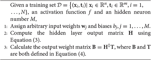
Algorithm 1 Extreme Learning Machine (ELM)

ELM provides a fast and efficient MLP training (Huang et al., 2006), but it needs to fix the number of hidden neurons to obtain a good generalization capability. In order to avoid the exhaustive search for the optimal value of M, several pruned methods have been proposed (Mateo and Lendasse, 2008; Miche et al., 2008a,b; Rong et al., 2008; Miche and Lendasse, 2009; Miche et al., 2010). Among them, the most commonly used is the ELM Optimally Pruned (OP-ELM) (Miche et al., 2010). The OP-ELM sets a very high initial number of hidden neurons (M≫N) and, by using Least Angle Regression algorithm (LARS) (Similä and Tikka, 2005), sorts the neurons according to their importance to solve the problem (Equation 2). The pruning of neurons is done by utilizing Leave-One-Out Cross-Validation (LOO-CV) and choosing the combination of neurons (which have been previously sorted by the LARS algorithm) that provides lower LOO error. The LOO-CV error is efficiently computed using the Allen's formula (Miche et al., 2010). For more detail, a summary of the OP-ELM algorithm is shown in Algorithm 2 (García-Laencina et al., 2011).

ALGORITHM 2

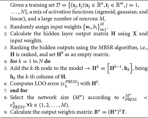
Algorithm 2 Optimally Pruned-ELM (OP-ELM)

Recently, a new method to design MLP architectures has been presented in Bueno-Crespo et al. (2013). It is called ASELM (“Architecture Selection Using Extreme Learning Machine”) and is based on the OP-ELM. Thus, once the initial MLP architecture is defined, the OP-ELM optimally discards those hidden neurons whose combination of input variables is not relevant to the target task. Because of the binary value of the input weights, the selection of hidden nodes implies also the selection of those relevant connections between the input and hidden layers. Thus, only input connections corresponding to selected hidden neurons and with input weights values equal to 1 will be part of the final architecture. A summary of the ASELM algorithm is shown below (Algorithm 3).

ALGORITHM 3

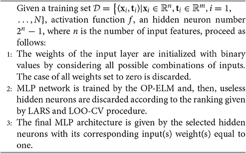
Algorithm 3 Architecture Selection ELM (ASELM)

3. Multitask Learning Architecture

The MTL architecture for a neural network is similar to the classical scheme STL (Single Task Learning). They differ in that MTL scheme has an output for each task to be learned, whereas STL scheme has a separate network for each one (Figure 1). Thus, when we speak about MTL, we are referring to a type of learning where a main task and other tasks (considered as secondary tasks) are learned all at once in order to help learning of the main one.

FIGURE 1

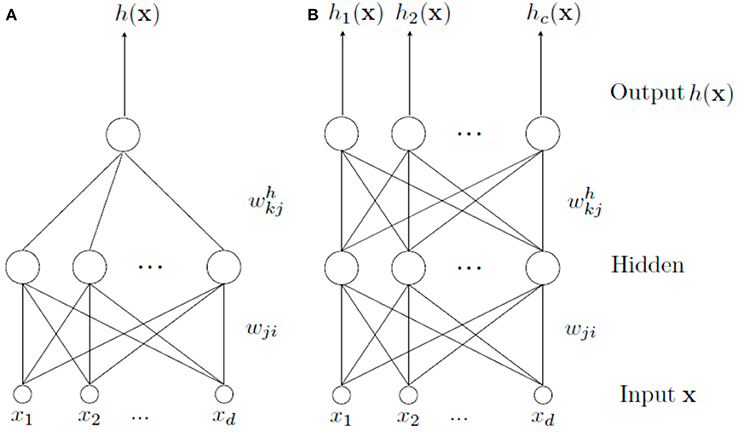
Figure 1. Different learning schemes. In (A), a STL architecture is shown. It is used to solve a single task alone. In (B), a set of tasks are learned simultaneously by means of a MTL architecture. In this case, there is a common part (from the input to the hidden layer) and a specific part (from the hidden layer to the output) for each task.

In a MTL scheme, there is a common part shared by all tasks and a specific one for each task. The common part is formed by the weights connections from the input features to the hidden layer, allowing common internal representation for all tasks (Caruana, 1993). Thanks to this internal representation, learning can be transferred from one task to another (Caruana, 1998). The specific part, formed by the weights that connect the hidden layer to the output layer, specifically allows modeling each task from the common representation. The main problem with this type of learning is to find tasks related to the main one. Even in case of finding them, it may be difficult to know the kind of relationship they have, because it can be a positive or negative influence to learn the main task.

4. Proposed Method

The method proposed in this paper is called MTL_ASELM since it is based on the ASELM to design MTL architectures. To do this, it is necessary to introduce a couple of modifications to the original method so as to adapt it to MTL. Firstly, the targets of secondary tasks will be used as new input features (removing them from the outputs of the classic MTL scheme) so that a similar architecture to that shown in Figure 1A is obtained. There is only a single output corresponding to the main task and an input vector composed now by the original input features and the targets of secondary tasks. This network is designed and trained using ASELM which, as it was commented before, realizes a selection of hidden nodes that implies also the selection of those relevant connections between the input and hidden layer. The selection of relevant secondary tasks is now performed since they are part of the input vector.

In a second stage, a MTL architecture is created. The secondary tasks selected in the previous stage as the most relevant to learn the main task are included as output components in the MTL neural network. A scheme of the proposed method can be seen in Figure 2.

FIGURE 2

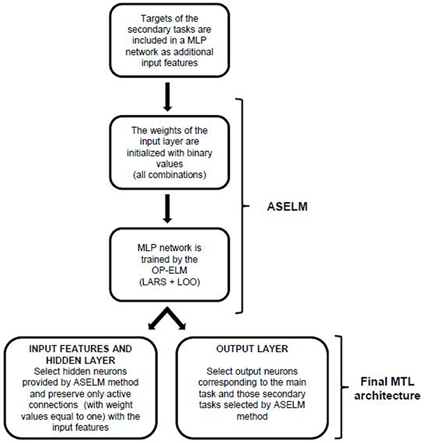
Figure 2. Flowchart of the proposed method.

This idea of exchanging outputs for inputs is not new. Caruana proposed that some inputs may work better as outputs, i.e., as new secondary tasks (Caruana, 1998). This idea is very interesting in machine learning and it has been used, for example, for developing efficient procedures to classify patterns with missing data (García-Laencina et al., 2010, 2013).

MTL_ASELM method allows pruning to take place both at the hidden layer and the output layer, at the same time that provides a unique solution. This uniqueness comes from the binary initialization of the hidden weights, which eliminates the random component thereof.

To further clarify the MTL_ASELM method, the following section includes an example of how the method is applied step by step to solve a particular problem (Logic Domain problem).

5. Experiments

In order to show the goodness of the MTL_ASELM method for designing an MTL architecture, results of classification test obtained with the single-task learning (STL), classic multitask learning (MTL), and MTL_ASELM have been compared. While the MTL_ASELM architecture is directly obtained by the proposed method, the best architecture for STL and MTL has been selected by cross-validation. For experiments, the three architectures are trained using the stochastic back-propagation with a cross-validation with 10-fold × 30 initializations. “Logic Domain,” “Monk's Problems,” “Telugu,” “Iris Data,” and “User Knowledge Modeling” datasets, will be used to show the performance of the method. These data sets are available at the UCI ML Repository (Asuncion and Newman, 2007), excepting “Logic Domain” problem (McCracken, 2003). Specific details about results for each dataset are described below.

“Logic Domain” dataset is used to see how MTL architecture is created by the MTL_ASELM method. This dataset is a toy problem specially designed for multitask learning. In this problem, targets are represented by the combination of four real variables (from seven inputs: x₁,…,x₇), considering the first task as the main task, and the others as secondary ones.

Table 1 shows the logical expression for each task. Note, that the main task (T_p) is only determined by the first four features of the problem. The secondary tasks share one or more variables with the main one. Nevertheless, only the second secondary task (T_Sec2) shares a common logic subexpression (x₃ > 0.5 ∨ x₄ > 0.5) with the main task.

TABLE 1

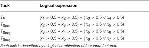
Table 1. Description of the “Logic Domain” tasks.

Initially, the neural network architecture is composed by M = 1023 (2ⁿ − 1, with n = 10; seven input features + three extra features corresponding to three secondary tasks) hidden units (see Figure 3). This suppose a large enough hidden layer number according to the ELM theory. Once this model is trained with ASELM method, the result is quite significant. The ASELM selects only two hidden neurons as the most relevant to learn the main task (Bueno-Crespo et al., 2013). By relevance order, these hidden weights are w₁₉₄ = [0 0 1 1 0 0 0 0 1 0] and w₇₆₈ = [1 1 0 0 0 0 0 0 0 0] corresponding to hidden neuron number 194 and 768, respectively. For simplicity, we will be referred to them as first neuron or w₁ and second neuron or w₂. From w₁, it can be observed that the first selected hidden neuron is only connected to input features x₃ and x₄, as well as the second secondary task (T_Sec2). From w₂, it follows that only x₁ and x₂ contribute to learning through their connection to the second hidden neuron (see Figure 3).

FIGURE 3

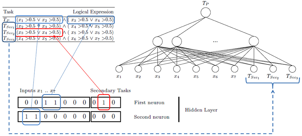
Figure 3. Logic Domain problem. Scheme to learn the main task using secondary tasks as inputs. 1023 neurons in the hidden layer have been generated. After ASELM is applied only two hidden neurons are selected whose weight vectors are shown in black boxes. The first neuron has three connections corresponding to the input features x₃ and x₄ and the second secondary task (T_Sec2). The second neuron is represented only by the input features x₁ and x₂.

This means that only T_Sec2 is influencing in the learning of the T_P through the first neuron that learns the input features x₃ and x₄, which is an expected result according to the previous comment indicating the relationship between T_p and T_sec2 (see Table 1). The second selected hidden neuron is only composed by the input features x₁ and x₂, without any input connection from the secondary tasks. Figure 4 shows the final architecture given by ASELM method.

FIGURE 4

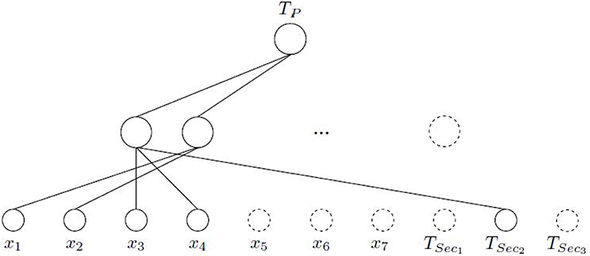
Figure 4. Logic Domain problem. Intermediate scheme where connections are pruned after ASELM. It can be observed how the input features x₅, x₆, and x₇, all hidden nodes least two, and secondary tasks T_Sec1 and T_Sec3 are removed because they are irrelevant for the learning of the T_P.

Next, a MTL architecture is created considering as outputs those corresponding to the main task and secondary ones selected in the previous stage. The latter are incorporated into the output layer preserving the connections established by the ASELM. In our case, only T_Sec2 has been selected. Figure 5 shows the final MTL_ASELM architecture. MTL_ASELM has removed the input features x₅, x₆, and x₇, and has selected only 2 neurons in the hidden layer from the 1023 neurons initially considered.

FIGURE 5

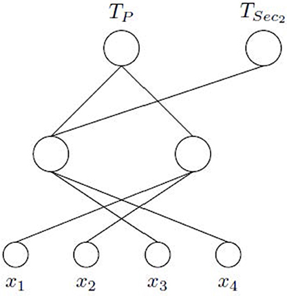
Figure 5. Logic Domain problem. Final architecture obtained with MTL_ASELM. T_P shares a hidden layer neuron with T_Sec2, which learns the common part of both tasks.

Figure 6 shows the MTL_ASELM schemes for other studied datasets. “Monk's Problems” dataset is a collection of three toy problems that present the same domain (six input features). In this problem, the targets associated to each task are described by the logical relations. Thus, Monk 1 (T_P) is described by (x₁ = x₂) ∨ (x₅ = 1); in Monk 2 (T_Sec1) exactly two identities from x₁ = 1, x₂ = 1, x₃ = 1, x₄ = 1, x₅ = 1, x₆ = 1 must be satisfied; and in Monk 3 (T_Sec2), (x₅ = 3 and x₄ = 1) or (x₅ ≠ 4 and x₂ ≠ 3) have to be fulfilled. MTL_ASELM selects 14 neurons in the hidden layer from a total of 255. Figure 6A presents the first five neurons and the last one for the selected architecture. For example, if we observe the first neuron, it connects the input feature x₅ with the outputs of T_P and T_Sec1, but not with T_Sec2. It can be observed that target associated to T_P and T_Sec1 match the value of x₅, what does not happen for T_Sec2.

FIGURE 6

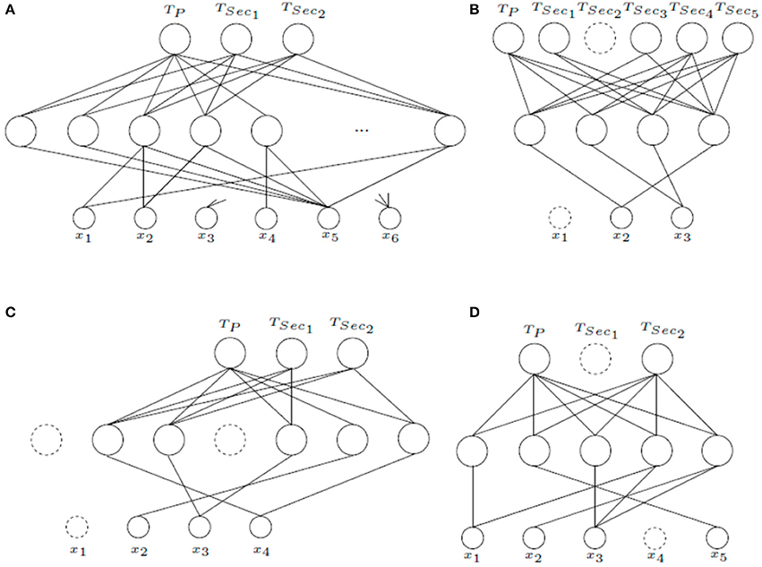
Figure 6. Final MTL_ASELM architectures for “Monk's Problems” (A), “Telugu” (B), “Iris Data” (C), and “User Knowledge Modeling” (D).

“Telugu” language dataset represents one of six languages designated a classical language of India. This datasets consists of three input features that represent language formants. For “Telugu,” MTL_ASELM selects 4 neurons in the hidden layer from a total of 255 initial neurons. Figure 6B shows the final architecture obtained. As can be seen, this architecture uses only two of the three input features, what is quite interesting because in dialects with fewer than six vowels, two formants are only required to classify (Pal and Majumder, 1977).

“Iris Data” (Figure 6C) represent a dataset of three types of flowers represented by four input features. For this dataset, 5 neurons are selected in the hidden layer from a total of 63 neurons. It can be observed that the input feature x₁ has been removed. The results show that the proposed method has a much more simplified architecture than classical multitask learning, although the classification test is similar due to the simplicity of the problem (see Table 2).

TABLE 2

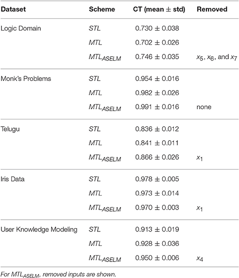
Table 2. Classification Test “CT” (mean ± standard deviation) with different schemes on several datasets.

“User Knowledge Modeling” (Figure 6D) is the real dataset about the students' knowledge status about the subject of Electrical DC Machines. The target is represented by four levels (very low, low, middle, and high). To give a multitasking approach a pairwise combination has been made (T_P = (very low ∨ low), T_Sec1 = (low ∨ middle), and T_Sec2 = (middle ∨ high)). It can be observed that T_Sec1 is removed. It is because T_Sec2 is more important to T_P, since T_Sec2 represents its opposite. Finally, 5 neurons are selected in the hidden layer from a total of 127 initial neurons.

Table 2 shows the classification accuracy results for all the data sets. Because the Logic Domain is an easy problem to solve for an MLP in an STL scheme, the number of samples has been reduced to 50 so that multitask learning can be appreciated. With all training samples, the result between STL and MTL_ASELM is practically invaluable. Taking into account this reduction of samples for the Logic Domain problem, MTL_ASELM presents better classification accuracy than STL and MTL. However, STL is better than the classic MTL, since MTL presents a completely interconnected scheme that is positively influenced by the related task (T_Sec2) and negatively by unrelated tasks (T_Sec1 y T_Sec3). This is not a general rule but it is an empirical result that shows that there are tasks that help the main task and others that are harmful.

For the rest of the data sets, the MTL_ASELM always provides the best results on average with a low standard deviation. This robustness in the solution is due to the particular initialization of the hidden weights that MTL_ASELM realizes.

To validate this assertion, a non-parametric statistical test has been performed. Specifically, the Wilcoxon Signed Ranks Test is used (Kruskal, 1957). A peer review has been performed. Comparing MTL_ASELM to STL, the p-value obtained is 0.078, which indicates that there are significant differences to 92%, being the best MTL_ASELM. Likewise, when applying the test with MTL_ASELM against classic MTL, the p = 0.080 indicates that there are significant differences to 92%, being MTL_ASELM better than MTL. However, there are no significant differences between STL and MTL, since the p = 0.683.

6. Discussion and Future Work

This paper presents a method to select tasks to be used in a MTL scheme providing information about weight connection, hidden nodes, input features, and most helpful secondary tasks for the learning of the main task. This method has been named MTL_ASELM because it is based on the ASELM algorithm (Bueno-Crespo et al., 2013), which proves to be an efficient method and single solution for the complete design of a MLP (input features, weights connections, and hidden nodes). By using secondary tasks as input features, MTL_ASELM applies the ASELM on the initial network which only has a single output corresponding to the main task. Thus, irrelevant nodes and connections are eliminated, what implies a selection of features (among which are the secondary tasks). After this stage, a final network is built with a dimension in the output layer equal to the number of secondary tasks selected as relevant plus one. Thus, the main drawback of multitask learning is eliminated, i.e., the negative influence of unrelated tasks. In addition, the modification of ASELM method to adapt it for a multitask scheme is achieved not only to eliminate connections from inputs features to hidden layer, but also from hidden to output layer. It is worth highlighting that, as well as ASELM, the MTL_ASELM method provides a single solution. This is due the fact that a binary initial selection of the hidden weights substitutes any random initialization process. Another important advantage is that it requires no parameter to be configured by the user. In the experiments section, it has been observed over real problems that the method MTL_ASELM gets a simplified solution with good generalization capabilities, in comparison to those obtained by a fully connected solution given by the classic MTL scheme.

Authors are working on extending the method to other learning models, such as Radial Basis Functions (RBF). Applying MTL_ASELM to regression problems is another research field since the ASELM is optimized for classification according to Huang et al. (2010). This limitation of the present method is due to the nature of ELM method, which is based on the pseudoinverse calculation. In this regard, we are working to use the sequential calculation pseudoinverse of Moore-Penrose (Van Heeswijk et al., 2011; Tapson and Van Schaik, 2013). Another line of research is to extend this method in the field of Deep Learning since new works on MultiTask Learning have lately appeared, most of them within the scope of Deep Learning (Liu et al., 2015; Thanda and Venkatesan, 2017).

Author Contributions

AB: Proposed method, software programming, experiments, reviews, results, and conclusions. RMML: Introduction, software programming, contributions of ideas and reviews. RME: Method description, contributions of ideas and reviews. JS: Work direction, architecture selection, contributions of ideas, reviews, conclusions, and future work.

Conflict of Interest Statement

The authors declare that the research was conducted in the absence of any commercial or financial relationships that could be construed as a potential conflict of interest.

The handling Editor declared a shared affiliation, though no other collaboration, with several of the authors RMML and JS, and the handling Editor states that the process met the standards of a fair and objective review.

Acknowledgments

This work has been supported by Spanish MINECO under grant TIN2016-78799-P (AEI/FEDER, UE). This paper is an extension of the one presented at the IWINAC 2015 conference (6th INTERNATIONAL WORK-CONFERENCE on the INTERPLAY between NATURAL and ARTIFICIAL COMPUTATION). Dedicated to the memory of Ph.D. Pedro José García-Laencina.

References

Asuncion, A., and Newman, D.-J. (2007). UCI Machine Learning Repository. Irvine, CA: Department of Information and Computer Science, University of California. Available online at: http://archive.ics.uci.edu/ml/

Google Scholar

Baxter, J. (1993). The evolution of learning algorithms for artificial neural networks. Complex Syst.

Google Scholar

Bueno-Crespo, A., García-Laencina, P. J., and Sancho-Gómez, J.-L. (2013). Neural architecture design based on extreme learning machine. Neural Netw. 48, 19–24. doi: 10.1016/j.neunet.2013.06.010

PubMed Abstract | CrossRef Full Text | Google Scholar

Bueno-Crespo, A., Menchón-Lara, R.-M., and Sancho-Gómez, J.-L. (2015). “Related tasks selection to multitask learning schemes,” in International Work-Conference on the Interplay between Natural and Artificial Computation (Elche: Springer), 213–221. doi: 10.1007/978-3-319-18833-1_23

CrossRef Full Text | Google Scholar

Caruana, R. (1995). Learning many related tasks at the same time with backpropagation. Adv. Neural Inform. Process. Syst. 7, 657–664.

Google Scholar

Caruana, R. (1998). “Multitask learning,” in Learning to Learn (Springer), 95–133.

Google Scholar

Caruana, R.-A. (1993). “Multitask connectionist learning,” in Proceedings of the 1993 Connectionist Models Summer School (Boulder).

Google Scholar

García-Laencina, P.-J., Bueno-Crespo, A., and Sancho-Gómez, J.-L. (2011). “Design and training of neural architectures using extreme learning machine,” in Neurocomputing: Learning, Architectures and Modeling, ed E. T. Mueller (Nova Science Publishers), 119–145.

García-Laencina, P.-J., Sancho-Gómez, J.-L., and Figueiras-Vidal, A.-R. (2010). Pattern classification with missing data: a review. Neural Comput. Appl. 19, 263–282. doi: 10.1007/s00521-009-0295-6

CrossRef Full Text | Google Scholar

García-Laencina, P.-J., Sancho-Gómez, J.-L., and Figueiras-Vidal, A.-R. (2013). Classifying patterns with missing values using multi-task learning perceptrons. Expert Syst. Appl. 40, 1333–1341. doi: 10.1016/j.eswa.2012.08.057

CrossRef Full Text | Google Scholar

Huang, G.-B., and Chen, L. (2007). Convex incremental extreme learning machine. Neurocomputing 70, 3056–3062. doi: 10.1016/j.neucom.2007.02.009

CrossRef Full Text | Google Scholar

Huang, G.-B., Ding, X., and Zhou, H. (2010). Optimization method based extreme learning machine for classification. Neurocomputing 74, 155–163. doi: 10.1016/j.neucom.2010.02.019

CrossRef Full Text | Google Scholar

Huang, G.-B., Wang, D., and Lan, Y. (2011). Extreme learning machines: a survey. Int. J. Mach. Learn. Cybernet. 2, 107–122. doi: 10.1007/s13042-011-0019-y

CrossRef Full Text | Google Scholar

Huang, G.-B., Zhu, Q.-Y., and Siew, C.-K. (2006). Extreme learning machine: theory and applications. Neurocomputing 70, 489–501. doi: 10.1016/j.neucom.2005.12.126

CrossRef Full Text | Google Scholar

Igelnik, B., and Pao, Y.-H. (1997). Stochastic choice of basis functions in adaptive function approximation and the functional-link net. IEEE Trans. Neural Netw. 8, 452–454.

PubMed Abstract | Google Scholar

Kruskal, W.-H. (1957). Historical notes on the wilcoxon unpaired two-sample test. J. Am. Stat. Assoc. 52, 356–360. doi: 10.1080/01621459.1957.10501395

CrossRef Full Text | Google Scholar

Liu, X., Gao, J., He, X., Deng, L., Duh, K., and Wang, Y.-Y. (2015). “Representation learning using multi-task deep neural networks for semantic classification and information retrieval,” in HLT-NAACL (Denver), 912–921. doi: 10.3115/v1/n15-1092

CrossRef Full Text | Google Scholar

Mateo, F., and Lendasse, A. (2008). “A variable selection approach based on the delta test for extreme learning machine models,” in Proceedings of the European Symposium on Time Series Prediction (Porvoo), 57–66.

Google Scholar

McCracken, P.-J. (2003). Selective Representational Transfer Using Stochastic Noise. Honurs thesis, Jodrey School of Computer Science, Acadia University.

Miche, Y., Bas, P., Jutten, C., Simula, O., and Lendasse, A. (2008a). “A methodology for building regression models using extreme learning machine: OP-ELM,” in Proceedings of European Symposium on Artificial Neural Networks (ESANN) (Bruges), 247–252.

Google Scholar

Miche, Y., and Lendasse, A. (2009). “A faster model selection criterion for OP-ELM and OP-KNN: Hannan-quinn criterion,” in European Symposium on Artificial Neural Networks (ESANN), Vol. 9 (Bruges), 177–182.

Google Scholar

Miche, Y., Sorjamaa, A., Bas, P., Simula, O., Jutten, C., and Lendasse, A. (2010). OP-ELM: optimally pruned extreme learning machine. IEEE Trans. Neural Netw. 21, 158–162. doi: 10.1109/TNN.2009.2036259

PubMed Abstract | CrossRef Full Text | Google Scholar

Miche, Y., Sorjamaa, A., and Lendasse, A. (2008b). “OP-ELM: theory, experiments and a toolbox,” in International Conference on Artificial Neural Networks (Prague: Springer), 145–154. doi: 10.1007/978-3-540-87536-9_16

CrossRef Full Text | Google Scholar

Pal, S.-K., and Majumder, D.-D. (1977). Fuzzy sets and decision making approaches in vowel and speaker recognition. IEEE Trans. Syst. Man Cybernet. 7, 625–629. doi: 10.1109/TSMC.1977.4309789

CrossRef Full Text | Google Scholar

Pao, Y.-H., Park, G.-H., and Sobajic, D.-J. (1994). Learning and generalization characteristics of the random vector functional-link net. Neurocomputing 6, 163–180. doi: 10.1016/0925-2312(94)90053-1

CrossRef Full Text | Google Scholar

Rong, H.-J., Ong, Y.-S., Tan, A.-H., and Zhu, Z. (2008). A fast pruned-extreme learning machine for classification problem. Neurocomputing 72, 359–366. doi: 10.1016/j.neucom.2008.01.005

CrossRef Full Text | Google Scholar

Serre, D. (2002). Matrices: Theory and Applications. Graduate Texts in Mathematics. New York, NY: Springer.

Google Scholar

Silver, D., and Mercer, R. (2001). “Selective functional transfer: Inductive bias from related tasks,” in IASTED International Conference on Artificial Intelligence and Soft Computing (ASC2001) (Cancum), 182–189.

Google Scholar

Similä, T., and Tikka, J. (2005). “Multiresponse sparse regression with application to multidimensional scaling,” in International Conference on Artificial Neural Networks, eds W. Duch, J. Kacprzyk, E. Oja, and S. Zadrożny (Heidelburg: Springer), 97–102.

Tapson, J., and Van Schaik, A. (2013). Learning the pseudoinverse solution to network weights. Neural Netw. 45, 94–100. doi: 10.1016/j.neunet.2013.02.008

PubMed Abstract | CrossRef Full Text | Google Scholar

Thanda, A., and Venkatesan, S.-M. (2017). Multi-task learning of deep neural networks for audio visual automatic speech recognition. arXiv:1701.02477.

Google Scholar

Van Heeswijk, M., Miche, Y., Oja, E., and Lendasse, A. (2011). GPU-accelerated and parallelized ELM ensembles for large-scale regression. Neurocomputing 74, 2430–2437. doi: 10.1016/j.neucom.2010.11.034

CrossRef Full Text | Google Scholar