Experience and Abstract Reasoning in Learning Backward Induction

Backward induction is a benchmark of game theoretic rationality, yet surprisingly little is known as to how humans discover and initially learn to apply this abstract solution concept in experimental settings. We use behavioral and functional magnetic resonance imaging (fMRI) data to study the way in which subjects playing in a sequential game of perfect information learn the optimal backward induction strategy for the game. Experimental data from our two studies support two main findings: First, subjects converge to a common process of recursive inference similar to the backward induction procedure for solving the game. The process is recursive because earlier insights and conclusions are used as inputs in later steps of the inference. This process is matched by a similar pattern in brain activation, which also proceeds backward, following the prediction error: brain activity initially codes the responses to losses in final positions; in later trials this activity shifts to the starting position. Second, the learning process is not exclusively cognitive, but instead combines experience-based learning and abstract reasoning. Critical experiences leading to the adoption of an improved solution strategy appear to be stimulated by brain activity in the reward system. This indicates that the negative affect induced by initial failures facilitates the switch to a different method of solving the problem. Abstract reasoning is combined with this response, and is expressed by activation in the ventrolateral prefrontal cortex. Differences in brain activation match differences in performance between subjects who show different learning speeds.

1. Introduction

Backward induction (BI) is a recursive algorithm, wherein inferences regarding a decision problem made at an earlier stage are applied to the process of deriving yet further inferences on the problem. As a mathematical construction, backward induction constitutes a benchmark of game theoretic rationality that prescribes the behavior of rational players in finite sequential games of perfect information. In game theory, the concept is at the basis of abstract theorems; most notably Zermelo’s, (1908, 1912) theorem on the existence of equilibria in pure strategies for those games, or Selten’s (1965) and Selten and Stoecker’s (1986) theorem characterizing Sub-game perfect equilibria.

In contrast to its applicability in mathematical proofs, backward induction has at times been considered inapposite as a descriptive account of the cognitive processes operating in human subjects during the sort of strategic interactions that game theorists would conceptually represent as sequential games (e.g., Fey et al., 1996; Aymard and Serra, 2001; Johnson et al., 2002). In part, backward inductive reasoning has been considered an unlikely description of the human thought process during such game situations, because it requires the cognitive enactment of a solution concept that is considerably complex and ostensibly unnatural. However, we find evidence that subjects playing the sequential game of perfect information in our experiment have a common pattern of learning the optimal solution, and that although individuals may differ in their speeds for producing this pattern, this path is common and reproduces the steps of the backward induction algorithm.

To argue effectively this conclusion, we first review what the backward induction algorithm prescribes. We illustrate backward induction in finite sequential games of perfect information. These are games in which players alternate in actions, know, and remember precisely the choices made by other players in previous stages of the game, and know exactly the payoff structure for all players involved. A strategy for a player is a rule assigning a move at every decision point. For these games, backward induction prescribes the following procedure to construct a strategy for every player: At the very last stage of the sequential game, when the final player makes the last choice of the game, she should move to maximize her payoff from the choice made at this stage. We can call this step the last stage. Since the game ends at the last stage, and because payoffs are known, rationality prescribes the outcome of the last player’s choice. In other words, all players, including the last player herself, can unambiguously determine what would constitute the payoff maximizing choice given the options available at the last stage. The second to last player should anticipate the unambiguous criteria according to which the last player will choose, and conclude that his second to last choice will ultimately yield the payoffs induced by the optimal move of the last player. After this has been established, the original game is effectively replaced by a game with shorter length where the last move is eliminated and the payoff at the last stage is defined to be the payoff following the optimal choice of the last player. Iterating this process until the initial decision point is reached produces a strategy for every player.

Backward inductive reasoning relies in an essential way on the human ability for recursive thought, which itself has been posited as a prerequisite for quintessential human achievements such as language acquisition and basic numeracy (Hauser et al., 2002). Hence, to the extent that this innate human ability to think recursively manifests itself in strategic games, there may indeed exist a link between fundamental cognitive processes in humans and the abstract game theoretic concept of backward induction. Following this conjecture, we conduct two studies of a particular strategic social interaction that facilitates recursive learning. These studies were designed to address two fundamental questions: First, what are the neural correlates of recursive learning in the strategic environment, and second, how do the cognitive processes involved in recursive learning connect to abstract backward inductive reasoning.

2. Experimental Paradigm

2.1. Hit-N Game

The finite sequential game which subjects play in our experiment is played by two parties on a virtual playing board, and is the same as used in Gneezy et al. (2010), Bouton (1901–1902), and Dufwenberg et al. (2009). The board used to display the game in the imaging study is presented in Figure 1.

FIGURE 1

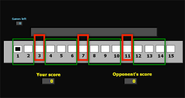
Figure 1. Board of positions for the game G(15, 3). This is the board of positions used in the imaging experiment. The superimposed red rectangles indicate the losing positions 3, 7, and 11. The green rectangles indicate the winning positions. In the lower section of the Figure 2 displays indicate the current score of the subject and the (computer) opponent.

For the basic variant of the Hit-N game used in this experiment, the first player to move is allowed to move a single common playing piece on the board, and she is allowed to move it only forward, by 1, 2, or 3 positions; no more or no less. The move then goes to the second player, who is allowed the same action of moving the figure 1, 2, or 3 positions forward. From thereon the opportunity to move according to the 1-2-or-3-only rule alternates between the two players. The player who reaches the final position (15 in experiment 1) first wins that game. We refer to this game as G(15, 3). A second game in our experiment involves the game G(17, 4) which is played on a virtual playing board of length 17, and allows players to move 1, 2, 3, or 4 positions forward.

We apply backward induction reasoning to this game to derive the optimal strategy: Players moving in position 12, 13, or 14 can win by reaching position 15 immediately. It follows that players moving at 11 have lost, since they can only move to 12, 13, or 14, where the opponent, as we have just seen, wins. Players can now replace the original game with the shorter game where the first player to reach position 11 wins: a move is optimal in the original game if and only if it is optimal in the reduced game. The same argument, repeated, shows that the player who first gets to position 7 wins; after which it can be concluded that the first to reach 3 wins. In summary, all positions different from 3, 7, and 11 are winning positions, because from there the player who is moving can reach either position 3, 7, or 11, and win: she just has to be sure to move there. On the other hand, positions 3, 7, and 11 are losing positions, and there is not much that the player moving there can do but hope for an error of the opponent. The argument we have just presented is the BI solution to G(15, 3). A similar argument shows that the losing positions in G(17, 4) are {2},{7}, {12}, and the groups of winning positions are {1}, {3, 4, 5, 6}, {8, 9, 10, 11}, {13, 14, 15, 16}.

2.1.1. The behavioral study

We use data from (Gneezy et al., 2010) as a behavioral sample, and focus here on error rate, response time, and their relation. A total of 72 subjects competed in 20 trials of G(15, 3), and 52 out of the 72 subjects played an additional 10 trials of G(17, 4).The incentive structure for G(15, 3) promised $5 for winning more than 5 trials over the 20 game period, and $20 for winning more than 11 trials. For G(17, 4) subjects were promised $10 for winning more than 5 games.

2.2. The fMRI Study

A total of 12 subjects participated in the MRI study. They played first 20 trials of G(15, 3), then 20 trials of G(17, 4) against a computer. The game, incentives, and instructions include three modifications to those used in the behavioral study. First, subjects are informed that they are playing a computer, programmed to win and subject to small errors. Also subjects play 20 trials of G(17, 4) (compared to 10 trials in study 1). Finally subjects were allowed 10 s to make a choice on each of their turns.

Data were collected at the Center for Magnetic Resonance Research (CMRR) at University of Minnesota using a 3-T Siemens Trio scanner. Both studies were approved by the Institutional Review Board (IRB) at the University of Minnesota. Subjects in both studies signed an informed consent form after they were given the instructions.

3. Model

To motivate the need for a theoretical model and the structure we are going to use, we begin by considering the relation between two key observable variables, response time and error rate. The response time is the length of the time interval between the moment in which the move of the opponent (another player or the computer) is observed and the moment in which the subject makes his next move. To define the error rate, we focus on G(15, 3) and note that at every winning position one, and only one, of the possible moves is correct, and the other two are incorrect. An error is the choice of the wrong move, and the error rate is the frequency of this event, conditional on the position being a winning position for the subject (these are the only positions at which an error is possible). The correct response rate is the difference from 1 of the error rate.

How are these two variables related? It may be reasonable to assume that, everything else being equal, a longer response time is associated with a higher correct response rate. This for example would be the case if the response time were varied exogenously, since by thinking about the problem for a longer time the subject would be more likely to achieve a richer understanding of what constitutes a good move. We point out that the condition of everything else being equal is crucial for this assertion. Considering now, that the length of the response time is not exogenous, but is decided upon by the subject who is reasoning about the decision, the relationship between response time and error rate may be different; indeed reversed: Since the reasoning activity can be assumed – in some measure – costly, a decision maker may compare and trade-off the estimated returns and costs from the reasoning activity. If the returns are estimated to be low, he may prefer to discontinue the process. If they are high, he might continue. Consider also, ability as an individual characteristic: An individual with lower cognitive skills may find the returns to his reasoning unsatisfactory, stop early, and be more likely to make the wrong choice. Similarly, a subject who has not acquired a basic familiarity with the game may conclude very little from his examination, stop cognitively engaging, and commit errors at a high rate. Both cognitive ability and problem familiarity are subsumed under the concept of ability. Considering response time as a choice variable together with differences in ability, the average relation at the individual level between response time and correct response rate may therefore be negative. In our data we find this to be the case. Figure 2 illustrates this point.

FIGURE 2

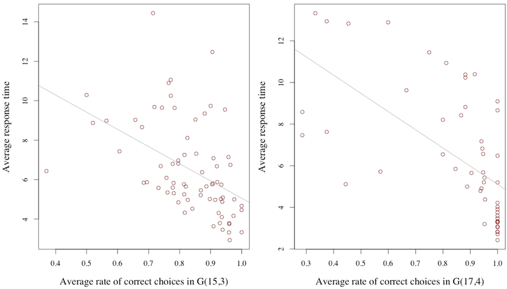
Figure 2. Average response time and average correct rate. The averages are computed for each subject over the trials for the G(15, 3) (on the left) and G(17, 4) on the right.

The simple regression in Table 1 of the correct response rate on the individual average response time confirms the negative relation, again in both games.

TABLE 1

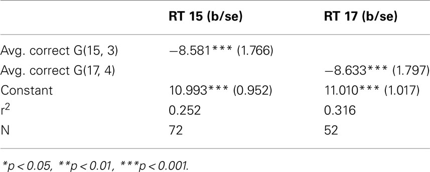
Table 1. Average response time and average correct rate OLS for both games.

Given the observed relation it appears particularly useful to consider a model in which response time is endogenously determined, and that reflects the notion that subjects choose to think about a problem, decide whether to stop thinking, and only then select a move.

3.1. Optimal Information Processing

In our experiment, at each turn, a player observes the position in the game, considers a set of potential cues and insights, and tries to identify the best move at the current position. At any point in time before choosing a move, he can terminate the process and then make a move determined by the conclusions reached up to this point. If he does not terminate the process, he has to decide the intensity of the effort devoted to the decision. The quality of his decision will then depend on his ability to reason about the game as well as his effort in doing so. We consider ability as an individual characteristic of the player, and this may describe both a player’s natural, general skills, as well as her acquired understanding of the game. We also consider effort as a choice variable. Ultimately, both effort and ability contribute positively to the agent’s problem solving success.

We model the above process as an optimal information acquisition problem to be solved in the time interval before the move. In the model, the subject has to choose an action, and has beliefs over which of the feasible actions [for example, the set {1, 2, 3} in G(15, 3)] in currently the best. In every instant during this process the agent can observe an informative signal on what the best action is, update her belief, and decide whether to continue the information acquisition process or to stop and choose what, given the current belief, is the optimal action. The model outlined above constitutes a general inter-temporal decision problem which can be formulated as a dynamic programming problem with an action set that consists of the agent’s effort and the decision to continue or stop processing information about the game. The state space of the problem is the set of beliefs over the action set, assigning to each action the probability that it is the best action. Information acquired in every instant is a partially informative signal on the true state; that is, on which among the feasible actions is the optimal one.

3.2. Model Predictions

It is clear that if ability is so low that any processed signal is entirely non-informative, the optimal time spent should be zero, and that correct response rates in this case will consequently be low. This is likely to occur in the early stages of the game, when subjects are just beginning to familiarize with the task, and lack even the basic insights to make even minor headway into the problem. At this stage we should observe a short response time and a high error rate. The effect should also be more pronounced at the difficult positions, those further from the end: this is because reasoning about the best move can only produce useful insights when the individual has some idea of what happens in later stages of the game, at positions closer to the end. In the initial rounds this understanding of the game at later stages is lacking, and the subject may prefer to discontinue the reasoning soon because it is not producing any useful insights.

At the opposite extreme, if ability is so large that the signal is completely informative, only a short time will be necessary while still leading to a high correct response rate. This is likely to occur of course at the late stages of the game, when a subject has an overall understanding of the optimal strategy. It is also likely to occur at the final positions, where very simple reasoning can provide the conclusion.

Between these two extremes, where signal is partly informative, the optimal policy will prescribe a positive response time. Overall the relation between ability and response time is non-monotonic: likely to be increasing for low values of ability, and decreasing for higher values.

A specific conclusion of the model is that the response time at a position is not necessarily monotonically increasing or decreasing with experience, but might instead be first increasing and then decreasing. At the early stages, low experience, which corresponds to low ability, induces an early stopping of the reasoning process (the information acquisition in our model), a short response time and a high error rate. At intermediate stages, as the subject acquires some basic understanding of the game, reasoning becomes more informative, hence stopping is postponed. Finally, in later periods the response time declines as subjects simply implement a solution algorithm which they now understand.

We will see that subjects’ behavior broadly matches these predictions, and provide the conceptual framework for the analysis of the imaging data.

4. Results

4.1. Behavioral Results

We review the basic behavioral results presented in Gneezy et al. (2010) to prepare for the analysis of the imaging data. To analyze error rate, we define a subject’s error j as a subject’s failure to move the marker to j, whenever this is possible and moving to j is part of the winning strategy. In G(15, 3) the possible errors of interest are failures to move the marker to any of the positions 3, 7, 11, or 15 whenever this would be possible. The error rate at j, e_j, is the fraction of times the error is made over the times the subject could avoid the error. For example e₃ is calculated as the number of times the subject had the opportunity of moving her opponent to position 3, yet failed to do so, divided by the times the subject held the move at position 1 or 2 in the game. The average error rate is the number of errors made at a winning position divided by the number of times the subject was in a winning position.

Response times for subjects show a marked decline across trials (see Figure 3), with subjects requiring more than 8 s on average to make a choice during the first three periods of the game, but not even half of that during the last 3 periods.

FIGURE 3

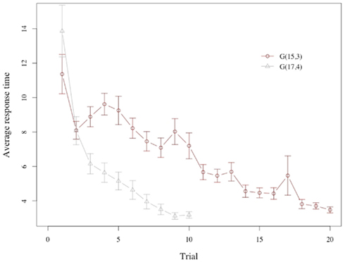
Figure 3. Response time. Average response time across trials in G(15, 3) and G(17, 4). The plot shows an unexpectedly long response time for the very first trial, which is driven by subjects’ response time at the initial onset of the game (see also Figure 7). At the onset of the game subjects appear to require additional time to familiarize themselves with the game environment. Removing the initial position of the initial round produces an increase in response time for G(15, 3) in line with model predictions.

There is a substantial difference in the evolution of the response time in the two games. Consider first the game G(15, 3): Note that the first trial has a very special role, since it is the one where subjects get acquainted with the task, and the rules of the game. If we ignore the first trial we see that the response time increases from the second to the fourth trial, and then declines, as the model predicts.

For the first trial of G(15, 3) the error rate is 0.38, which is significantly lower than the average error rate that would be expected if choices were made randomly. Across 20 trials of study 1, the error rate steadily declines until it almost reaches zero: see Figure 4.

FIGURE 4

Figure 4. Error rate by period. Average error by type for G(15, 3).

The four possible errors in G(15, 3) occur at significantly different rates. No subject deviates from the winning strategy choice at the final 3 positions (e₁₅ = 0). Error rates and average period marking the last occurrence of a particular error are lower for positions closer to the game’s end (e₃ ≥ e₇ ≥ e₁₁): see Figure 5.

FIGURE 5

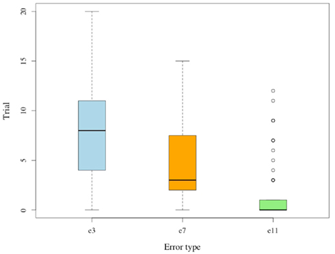
Figure 5. Last trial for error. Whisker plot of trial during which the last error occurred; separated by type.

Each of the differences between e₃, e₇, and e₁₁ is statistically significant (p < 0.01), and the pattern suggests that subjects indeed learn to identify losing positions in a sequential manner that begins from the game’s final positions. These observations indicate that subjects progress through a sequence of minor realizations toward becoming proficient in the Hit game. The above trends for G(15, 3) replicate in G(17, 4). For both games we observe lower error rates at later positions, and an overall decrease of error rates over repeated trials. Average response times decline across trials in both games.

Subjects make significantly fewer mistakes in G(17, 4) than in G(15, 3) indicating that subjects transfer some of their acquired skill to the new game. Observing however, that only 20 out of 72 subjects manage to commit zero errors in G(17, 4), it is likely, that most subjects have not fully developed the explicit BI solution to the sequential game after 20 trials of G(15, 3).

Figure 6 illustrates the average response time in the losing positions, for each of the periods.

FIGURE 6

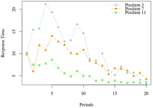
Figure 6. Response times in losing positions, G(15, 3). For each of the 20 periods in which the game G(15, 3) was played we report the average response time at each of the losing positions, 3, 7, and 11.

For position 11, the losing position which is closest to the end, the highest response time occurs in the first period, and declines in the periods thereafter. The peak for position 7 is reached at period 4, and that for position 3 is reached at period 5. As the model predicts, the response time is non-monotonic over the periods. For example the response time in period 7 is low at the initial stages, when subjects typically have a limited understanding of the game, but increases as the insight that the position 11 is a losing position is acquired and becomes available in the analysis of what to do at position 7. In later periods the response time at position 7 declines.

A similar relation can be seen in Figure 7, which illustrates the average response time at winning positions for G(15, 3).

FIGURE 7

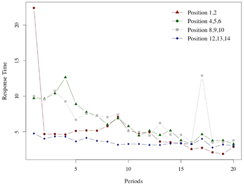
Figure 7. Response times in winning positions. As in the previous Figure 6 we report for each of the 20 periods in which the game G(15, 3) was played the average response time at each of the four winning positions groups.

In this case too, the peak for the middle positions (winning positions {4, 5, 6} and {8, 9, 10}) is reached after an initial low value. The peak is reached at period 4 for {4, 5, 6} and at period 3 for {8, 8, 10}. The response time at the very first positions {1, 2} increases slowly; the maximum is reached at period 8, after an initial spike in period 1 which is likely to be due to the fact that the very first instance of position 1 is also the subjects’ very first encounter with the game. The response time at the easy positions {12, 13, 14} monotonically declines after the initial period.

The figures we have seen present instructive average values over individuals’ response times. A more accurate description is provided by the panel data regressions in Table 2 for G(15, 3) game and Table 3 G(17, 4) for which the dependent variable is the response time and the time variable for the panel is the index of the period. The independent variables are dummy variables corresponding to the groups of positions. They are indexed in increasing order according to their position on the board, left to right. For example, the first group of winning positions (Win Pos 1) in game G(15, 3) indicates the set of positions {1, 2}. The second group of losing positions for G(17, 4) indicates the position 7. In both regressions the variable dropped is the final group of winning positions, that is {10, 11, 12} for G(15, 3) and {13, 14, 15, 16} for G(17, 4).

TABLE 2

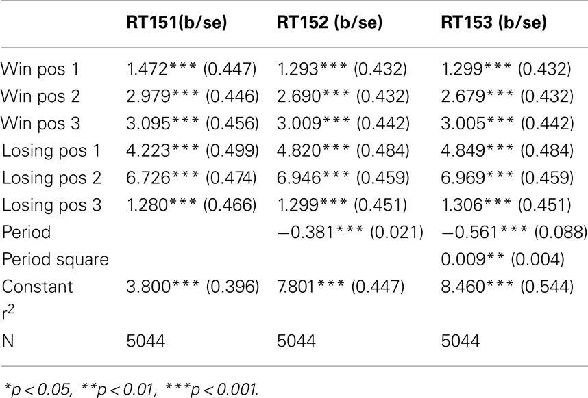
Table 2. Response time in G(15, 3): panel data analysis.

TABLE 3

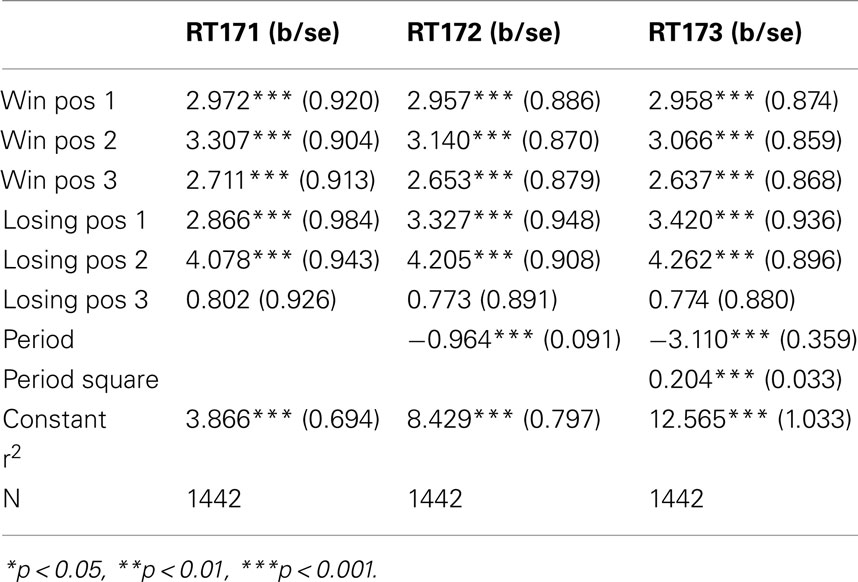
Table 3. Response time in G(17, 4): panel data analysis.

The constant value is similar in both games, and around 4 s. The main effect of learning the game is estimated by the variables period and period square, indicating a significant and fast [particularly in the game G(17, 4)] decline over time. The other variables confirm what we have seen in the aggregate analysis of the figures. Most notably, the increase in response time at losing positions is significantly higher than the one induced by winning positions; making more likely the conjecture that subjects carry over into the analysis of positions further from the end, insights they have obtained from the losing position 11, and possibly search for equivalent insight among positions earlier in the game.

4.2. The FMRI Data

4.2.1. Expected activation patterns and regions of interest

On the basis of the model and the analysis of the behavioral data we can formulate hypotheses to be tested in the study of the imaging data.

Learning of the method of backward induction should begin with the negative affective response experienced with moving at position 11, and realizing that the game is lost at that point. This experience should involve the reward system, particularly the Striatum (Schultz et al., 1997). We explore this hypothesis in section 4.3.

The predicted striatal response should be stronger, and occur earlier with subjects for whom behavioral evidence indicates that they posses a better understanding of the optimal strategy. We explore this hypothesis in section 4.4.

Further, the analysis of behavioral data has shown longer response times at the losing positions of game G(15, 3). The brain activation at these three positions should be similar, but should occur at different points in time during the experimental session. Brain activation should involve both areas associated with reward system and areas involved in abstract reasoning. We test this hypothesis in section 5 (see in particular in Figure 11).

One of our main assertions is, that the affective response induced by the understanding that the game is lost at position 11 should occur together with activation of frontal areas involved in planning, particularly VLPFC (Crescentini et al., 2011). This hypothesis is also examined in section 4.5.

In what follows we present results obtained from an event-related random effects general linear model (rfxGLM) with 16 predictors. Predictors are dummy variables indicating the 7 sets of positions for G(15, 3) over the first 10 trials (Early) and the last 10 trials (Late). A dummy variable indicating the computer’s turn, and a constant term complete the model. The omitted variable corresponds to a resting period between trials. Unless explicitly stated, all results reported here are significant at an uncorrected threshold of p ≤ 0.005; t(11) ≥ 3.59 for the full sample, or with t(5) ≥ 4.77 when split into Fast and Slow Learners. Fast Learners are defined as the 6 subjects with the lowest average error rate over both games. These are incidentally also the 6 subjects with the most wins in G(15, 3). Correspondingly, Slow Learners are the 6 subjects with the highest average error rates.

The model and observed behavior suggests that subjects become proficient at the Hit-15 game via a sequence of insights pertaining to their experience at losing positions; the generic manifestation of which is the avoidance of the losing position at 11, followed by avoidance of position 7, and for some subjects avoidance of position 3. These adaptations, which are likely accompanied by (conscious) realization of these positions as losing positions happen at dramatically varying rates between subjects, and have critical relation to models of prediction error processing and temporal difference learning (see e.g., Schultz et al., 1997, or Daw et al., 2010). According to models of prediction error-based learning, unexpected occurrences of losing positions should be accompanied by corresponding BOLD signal change in areas involved with prediction error (PE) tracking, such as the Striatum (Schultz et al., 1997) and Insula (Preuschoff et al., 2008). We expect to see these PE responses whenever subjects first realize that a given position is a losing position, and also when subjects are unexpectedly placed onto an already identified losing position; both of which necessitate a yet incomplete understanding of the game, when played against a reasonably proficient opponent such as the computer program used for this study. This expectation follows, because prediction error responses should become less pronounced as subjects gain greater insight into the game as a consequence of their increased ability to accurately predict the games outcome. Hence, once the game’s losing positions have been identified, finding oneself at a subsequent losing position becomes almost perfectly predictable at earlier stages, wherefore prediction errors should eventually approach zero.

4.3. Prediction Error Response in the Striatum and Insula

All subjects in the fMRI sample learn to identify position 11 as a losing position at some point during the game. In agreement with the idea that the identification of position 11 as a losing position induces an activation in the reward system, we find significant differences in striatal activation for subjects considering a move at losing position 11 compared to when considering a move at winning position {1, 2}. The difference in activation is in the direction of a negative prediction error, and an illustration is provided in Figure 8. (See also Appendix for time course graphs of BOLD activation).

FIGURE 8

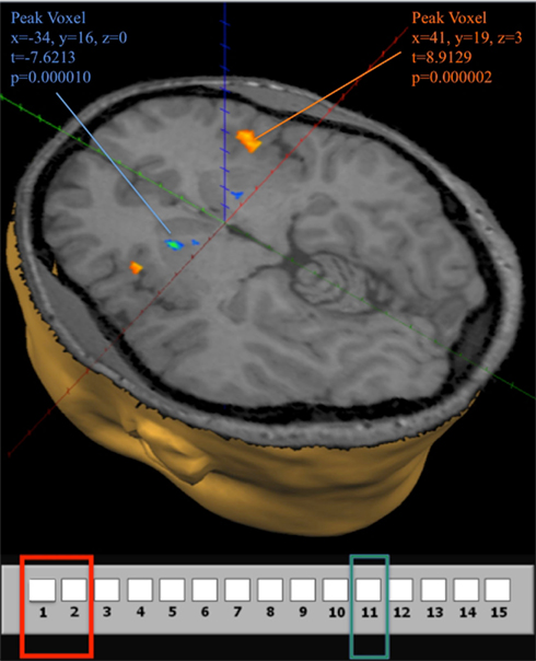
Figure 8. Brain activity at the losing position 11 in G(15, 3). Contrast obtained from a GLM with 16 predictors on all 12 subjects. In the GLM we use the same 7 groupings for positions in the game, and differentiate between positions during the first (early) and last (late) 10 trials, for a total of 14 predictors. An additional predictor for computer choices and a constant term describe the full model. The contrast used in the figure shows activation when the current position is 11 during both early and late trials compared to activation at positions {1, 2} during early and late trials. The map shows activation at a false discovery rate q < 0.05.

Figure 8 also shows significant positive activation of the left and right Insula at coordinates (41, 19, 3), as subjects perceive the near inevitability of losing the game at position 11. This activation is consistent with the Insula’s involvement in processing negative affect, and it’s role in signaling negative prediction errors (Seymour et al., 2004)

4.4. Prediction Error Response for Fast Learners

Given our main interest in the neural signature of the sequential, recursive way in which subjects learn the solution to the Hit-N game, we concentrate in Figure 9 on the Fast Learners; those subjects who actually manage to quickly reduce the amount of errors they make in the game.

FIGURE 9

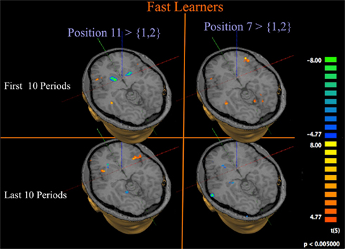
Figure 9. Progression of activation at losing position 11 for fast learners. GLM and contrasts as for Figure 8, but limited to Fast Learners.

The left panel of Figure 9 contrasts activation at position 11 to activation at position {1, 2} for Fast Learners. Consistent with the role of the Striatum in signaling prediction errors, we find that subjects show a strong initial negative response in the Striatum at losing position 11 during the first 10 rounds, which diminishes or disappears during the last 10 rounds. Figure 10C shows that this change of Striatal activity for Fast Learners is statistically significant at an uncorrected threshold of p ≤ 0.005, [t(5) ≥ 4.77]. At the same threshold, we observe significant activity in the Insula during both time periods.

FIGURE 10

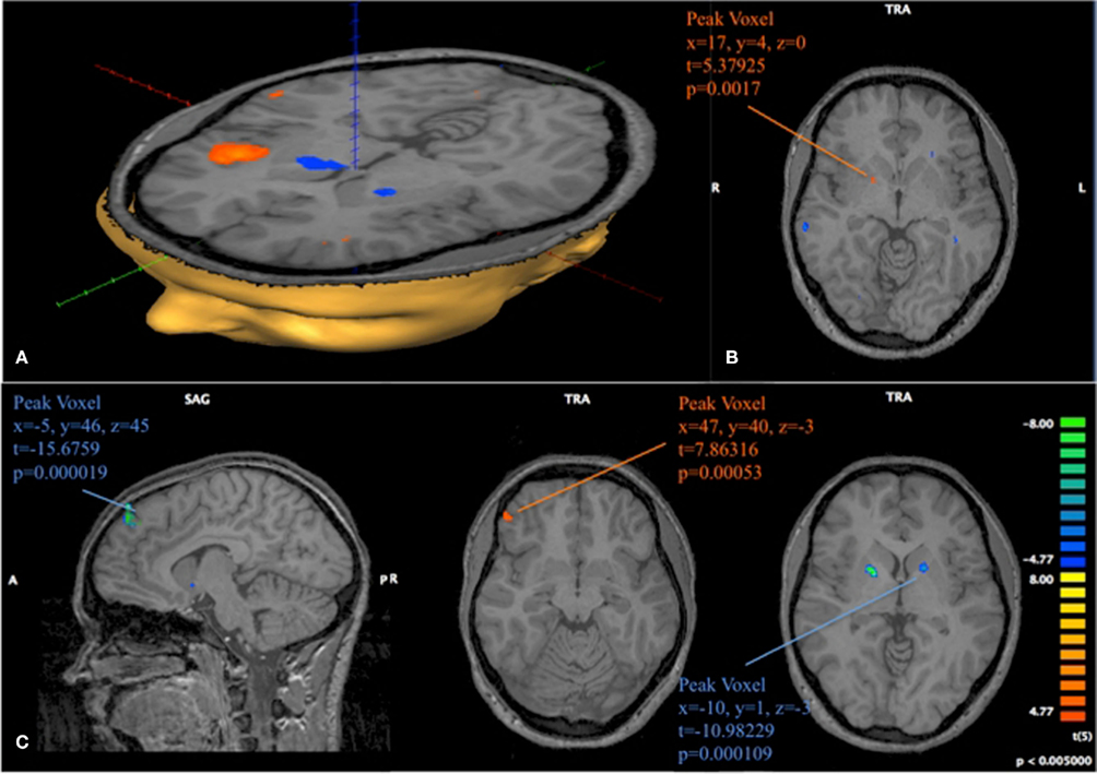
Figure 10. Progression of activation in fast and slow learners. (A) Contrast obtained from a GLM with 16 predictors on 6 subjects classified as Slow Learners. The depicted contrast shows activation at position 11 compared to activation at position 1, 2 during late trials. p < 0.005 uncorrected, t > 4.77. (B) Same model as (A). The depicted image subtracts the contrast obtained for positions 11 vs {1, 2} in late periods from the contrast obtained for those positions during early periods. Positive identification of Striatum in this contrast, is driven by a more strongly negative activation at position 11 in late periods for Slow learning subject. (C) 12 predictor GLM for 6 subjects classified as Fast Learners. As in (B), we show the subtraction of the contrast (11 early-1, 2 early)–(11 late-1, 2). We find activation in Medial Prefrontal Gyrus (MPFG), VLPFC, and Striatum. Negative identification in Striatum is driven by a more strongly negative response at position 11 during early trials for Fast Learners. p < 0.005 uncorrected for all images depicted here.

Our analysis also shows strong activity in the Insula at position 7 compared to {1, 2} during early trials, and eventually activity in the Striatum at position 7 during late trials; indicating a shift of the prediction error from position 11 to position 7; the sequence – as we have already shown – in which subjects learn the losing positions.

Figure 10 provides support to the above observations by overlaying the contrasts of early and late activity at position 11 (compared to {1, 2}) for both Fast and Slow learners. Slow learners exhibit detectable striatal activation in direction of a prediction error only during the last 10 trials; consistent with the observation that these subjects learn the game according to the same general pattern, but at a slower pace, than subjects classified as Fast Learners. However, the direct test of the effects of Early/Late periods, Fast/Slow learners, and the interaction term of these classifications, shown in Table 4, did not identify a statistically significant effect for the interaction (p = 0.158).

TABLE 4

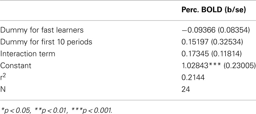
Table 4. Interaction between fast/slow learner, and early/late trial on BOLD signal contrast position 11 – position {1, 2} in Striatum.

4.5. Experience-based Learning and Abstract Reasoning

The center image of Figure 10C identifies a cluster of voxels in the ventrolateral prefrontal cortex (VLPFC; 47, 40, 3) with strong positive activation during the early losing position for Fast Learners. We are left to investigate the activity in this area when subjects are in losing positions for the game G(15, 3).

Our analysis of losing positions, illustrated in Figure 11, shows statistically significant increases of activation in the VLPFC at all of the losing positions during G(15, 3). Given this region’s association with tasks requiring spatial imagery in deductive reasoning (see Knauff et al., 2002 or Crescentini et al., 2011) the observation of higher activity during losing positions is of particular interest, as it indicates the special contribution that the experience of a losing position seems to make toward subject’s progress in learning the game.

FIGURE 11

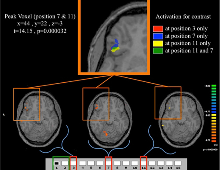
Figure 11. Fast learners at the losing positions. Contrast for Fast Learners during first 10 periods at p < 0.005. The contrasts used are for each of the three losing position, compared to the predictor given by the game being in position {1, 2}. For example the contrast for the position 3 indicates the comparison between position 3 and position {1, 2}. The top panel shows the clusters in VLPFC activated for the different contrasts. The lower panel shows the activation for the contrasts (3,{1, 2}), (7,{1, 2}), and (11,{1, 2}). Activation in VLPFC is not found in Fast Learners during the last 10 rounds, and Slow Learners show it only during the last 10 rounds for 11-{1, 2}. As shown in Figure 5, Fast Learners do not make mistakes past round 10, while Slow Learners commit mistakes even at position e11 past round 10. It should be also noted here that a direct test of the interaction between subjects’ categorization as Fast/Slow Learner and a dummy variable indicating Early/Late trials did not yield a statistically significant effect (p = 0.158 two-sided, see Table 4). We believe that the failure to identify such an effect at conventional significance level in our data may be due to small sample size, and an insufficiently precise measure of when subjects learn the game.

Figure 11 shows overlapping regions of activation for all losing positions experienced by Fast Learners that is most pronounced at position 11, and least pronounced at position 3; once again highlighting the critical nature of the initial losing position 11 for subject’s learning experience with the game.

5. Conclusion

We have explored how subjects learn to play the Hit-N game, and how this process converges for all subjects to learning the optimal strategy with the method of backward induction. We found strong evidence for a sequential learning process in which subjects learn the losing positions at the game’s end first. We showed that the behavioral characteristics (in error rate and response time) of this sequential learning process are consistent with a basic search model in which subjects choose an optimal search effort conditional on their ability and associated search costs.

We have also shown a neural pattern of activation in the brain’s reward system, including the Insula and Striatum, that mirrors the behaviorally implied pattern of subjects learning to identify losing positions from the game’s end. In particular, we find that the rate at which subjects learn to identify losing positions is also reflected by a differential onset of prediction error response between Fast and Slow Learners. A critical finding of our study is the implication of the prefrontal cortex in subject’s progression toward finding the solution to the Hit-N game. Here we find that activity in VLPFC is higher at losing positions than at corresponding winning positions. Taken together, these findings point toward a cognitive process in which the affective experience of a losing position feeds critically into the subject’s abstract cognitive engagement with the task.

While most of our discussion concentrated on subject’s success in recursively learning to identify losing positions in the Hit-N game, it is clear that such a process – although enabling subjects to master any length Hit-N game – is not equivalent to an abstract, explicit understanding of the BI solution to the game; one which could be transferred instantaneously to other similar games, such as G(17, 4). We see then, in both of our studies, that most subjects, despite quickly becoming highly proficient in G(15, 3), fail to instantaneously achieve proficiency in G(17, 4). Instead, subjects require an abbreviated learning period also for the second game.

What seems remarkable about the transition of behavior from G(15, 3) to G(17, 4) is that subjects, even without ostensibly having explicit knowledge of the BI solution at the time they begin G(17, 4), nonetheless commit fewer errors, and require a shorter learning phase for the theoretically more difficult second game. This observation provides strong indication that the recursive learning algorithm that enables learning of G(15, 3) is also a contributor to the development of a precursory understanding of the game’s abstract solution. One implication of this finding is that complex cognitive insights, such as understanding that backward inductive reasoning provides a solution to the general Hit-N game, can arise from the interaction of experience-based reward system responses and abstract reasoning within a relatively simple model. The fact that an experience-based understanding derived from playing G(15, 3) is effective in improving subject’s performance in G(17, 4) suggests that at least some higher-order cognition and insights might be motivated and prepared by joint activity in the brain’s reward system and prefrontal cortex.

6. Materials and Methods

6.1. MRI Data Acquisition

High resolution anatomical images were acquired first, using a Siemens t1-weighted 3D flash 1 mm sequence. Then, functional images were acquired using echo planar imaging with Repetition Time (TR) 2000 ms, Echo Time (TE) 23 ms, flip angle 90°, 64 × 64 matrix, 38 slices per scan, axial slices 3 mm thick with no gap. The voxel size was 3 mm × 3 mm × 3 mm.

The data were then preprocessed and analyzed using Brain Voyager QX 2.1. The anatomical images were transformed into Talairach space in 2 steps: first the cerebrum was rotated into anterior commissure – posterior commissure (AC-PC) plane using trilinear transformation, second we identified 8 reference points (AC, PC, and 6 boundary points) to fit the cerebrum into the Talairach template using trilinear transformation. We preprocessed functional data by performing slice scan time correction, 3D movement correction relative to the first volume using trilinear estimation and interpolation, removal of linear trend together with low frequency non-linear trends using a high-pass filter. Next, we co-registered functional with anatomical data to obtain Talairach referenced voxel time courses, to which we applied spatial smoothing using a Gaussian filter of 7 mm.

GLM Models

fMRI analysis was performed in Brain Voyager QX version 2.1. Contrasts obtained for G(15, 3) are based on the results of an event-related general linear model with random effects using 16 predictors. Seven predictors signify the period in which a subject contemplates any of the positions {1, 2}, {3}, {4, 5, 6}, {7}, {8, 9, 10}, {11}, {12, 13, 14} during the first 10 trials of G(15, 3). Another 7 predictors signify the same position during the last 10 trials. An additional predictor for times in which the computer is moving and an intercept term describe the model. Contrasts obtained for G(17, 4) are based on the results of an event-related general linear model with random effects using 16 predictors. Seven predictors signify the period in which a subject contemplates any of the positions {1}, {2}, {3, 4, 5, 6}, {7}, {9, 10, 11}, {12}, {13, 14, 15, 16} during the first 10 trials of G(17, 4). Another 7 predictors signify the same position during the last 10 trials. An additional predictor for times in which the computer is moving and an intercept term describe the model.

6.3. Fast and Slow Learners

The fMRI study consists of 12 subjects. For analysis comparing Fast and Slow Learners in G(15, 3), subjects were split into groups according to their overall error rate (a subject is slow if the error rate is larger than 40%), which also constitutes a splitting according to Wins in G(15, 3) (a subject is slow if the number of wins in that game is less than five). Both are median values, but they are also values at which there is a large change of performance.

Conflict of Interest Statement

The authors declare that the research was conducted in the absence of any commercial or financial relationships that could be construed as a potential conflict of interest.

Acknowledgments

We thank audience at several seminars and conferences. The research was supported in part by the NSF grant SES 0924896 to Aldo Rustichini.

References

Aymard, S., and Serra, D. (2001). Do individuals use backward induction in dynamic optimization problems? An experimental investigation. Econ. Lett. 73, 287–292.

Bouton, C. (1901–1902). Nim, a game with a complete mathematical theory. Ann. Math. 3, 35–39.

Pubmed Abstract | Pubmed Full Text | CrossRef Full Text

Crescentini, C., Seyed-Allaei, S., De Pisapia, N., Jovicich, J., Amati, D., and Shallice, T. (2011). Mechanisms of rule acquisition and rule following in inductive reasoning. J. Neurosci. 31, 7763–7774.

CrossRef Full Text

Daw, N. D., Gershman, S. J., Seymour, B., Dayan, P., and Dolan, R. J. (2010). Model-based influences on humans’ choices and striatal prediction errors. Neuron 69, 1204–1215.

CrossRef Full Text

Dufwenberg, M., Sundaram, R., and Butler, D. (2009). Epiphany in the game of 21. J. Econ. Behav. Organ. 75, 132–143.

CrossRef Full Text

Fey, M., McKelvey, R., and Palfrey, T. (1996). An experimental study of constant-sum centipede games. Int. J. Game Theory 25, 269–287.

CrossRef Full Text

Gneezy, U., Rustichini, A., and Vostroknutov, A. (2010). Experience and insight in the race game. J. Econ. Behav. Organ. 75, 144–155.

Pubmed Abstract | Pubmed Full Text | CrossRef Full Text

Hauser, D., Chomsky, N., and Fitch, W. T. (2002). The faculty of language: what is it, who has it, and how did it evolve? Science 298, 1569–1579.

CrossRef Full Text

Johnson, E. J., Camerer, C., and Sen, S. (2002). Detecting failures of backward induction: monitoring information search in sequential bargaining. J. Econ. Theory 104, 16–47.

CrossRef Full Text

Knauff, M., Mulack, T., Kassubek, J., and Salih, H. R. (2002). Spatial imagery in deductive reasoning: a functional MRI study. Cogn. Brain Res. 13, 203–212.

Pubmed Abstract | Pubmed Full Text | CrossRef Full Text

Preuschoff, K., Quartz, S. R., and Bossaerts, P. (2008). Human insula activation reflects risk prediction errors as well as risk. J. Neurosci. 28, 2745–2752.

Pubmed Abstract | Pubmed Full Text | CrossRef Full Text

Schultz, W., Dayan, P., and Montague, P. R. (1997). A neural substrate of prediction and reward. Science 275, 1593–1598.

Selten, R. (1965). Spieltheoretische behandlung eines oligopolmodells mit nachfragetragheit. Z. Gesamte Staatswiss. 12, 301–324.

CrossRef Full Text

Selten, R., and Stoecker, R. (1986). End behavior in sequences of finite prisoner’s dilemma supergames. J. Econ. Behav. Organ. 7, 47–70.

Pubmed Abstract | Pubmed Full Text | CrossRef Full Text

Seymour, B., O’Doherty, J. P., Dayan, P., Koltzenburg, M., Jones, A. K., Dolan, R. J., Friston, K. J., and Frackowiack, R. S. (2004). Temporal difference models describe higher-order learning in humans. Nature 429, 664–667.

CrossRef Full Text

Zermelo, E. (1908). Neuer Beweis für die Möglichkeit einer Wohlordnung. Math. Ann. 65, 107–128.

Zermelo, E. (1912). “Über eine Anwedung der Mengenlehre auf die Theorie des Schachspiels,” in Proceedings of the Fifth International Congress of Mathematicians, Vol. II (Cambridge: Cambridge University Press), 501.

Appendix

The following figures show time series plots of percentage BOLD signal change in the game G(15, 3) for clusters defined by the contrast of positions 11-{1, 2}, using t = 4.5, cs = 100. The x-axis represents positions in G(15, 3).

In graphs comparing early (first 10) and late (last 10) trials, error bars are for the mean condition over all 20 trials.

FIGURE A1

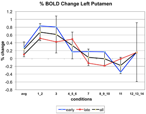
Figure A1. Time series of percentage BOLD change for G(15,3).

FIGURE A2

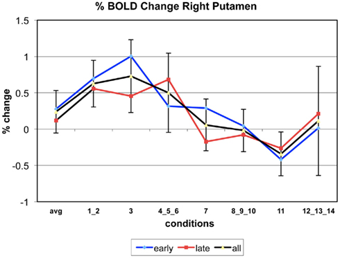
Figure A2. Time series of percentage BOLD change for G(15,3).

FIGURE A3

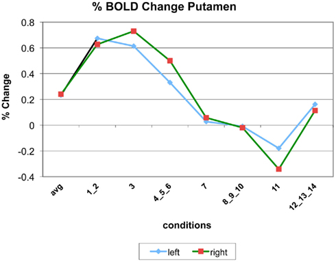
Figure A3. Time series of percentage BOLD change for G(15,3).

FIGURE A4

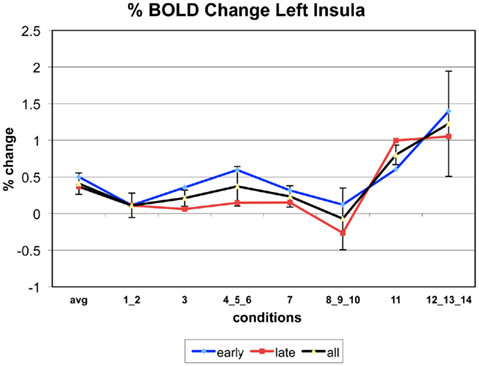
Figure A4. Time series of percentage BOLD change for G(15,3).

FIGURE A5

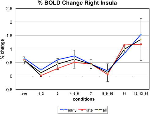
Figure A5. Time series of percentage BOLD change for G(15,3).

FIGURE A6

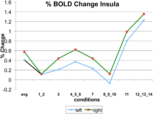
Figure A6. Time series of percentage BOLD change for G(15,3).

FIGURE A7

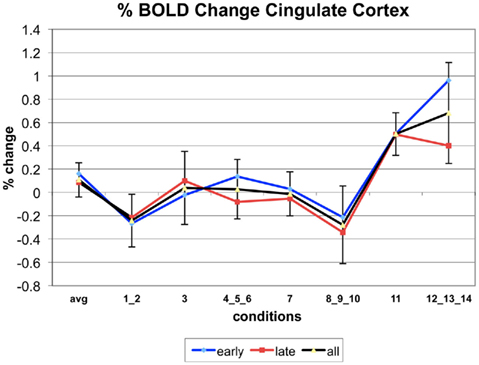
Figure A7. Time series of percentage BOLD change for G(15,3).