 Juemin Yang
 Lior Shmuelof
 Luo Xiao1
 John W. Krakauer
 Brian Caffo
- 1Department of Biostatistics, Bloomberg School of Public Health, Johns Hopkins University, Baltimore, MD, USA
- 2Department of Brain and Cognitive Sciences, Ben-Gurion University of the Negev, Beersheba, Israel
- 3Departments of Neurology and Neuroscience, Johns Hopkins University, Baltimore, MD, USA
A methodology for investigating learning is developed using activation distributions, as opposed to standard voxel-level interaction tests. The approach uses tests of dimensionality to consider the ensemble of paired changes in voxel activation. The developed method allows for the investigation of non-focal and non-localized changes due to learning. In exchange for increased power to detect learning-based changes, this procedure sacrifices the localization information gained via voxel-level interaction testing. The test is demonstrated on an arc-pointing motor task for the study of motor learning, which served as the motivation for this methodological development. The proposed framework considers activation distribution, while the specific proposed test investigates linear tests of dimensionality. This paper includes: the development of the framework, a large scale simulation study, and the subsequent application to a study of motor learning in healthy adults. While the performance of the method was excellent when model assumptions held, complications arose in instances of massive numbers of null voxels or varying angles of principal dimension across subjects. Further analysis found that careful masking addressed the former concern, while an angle correction successfully resolved the latter. The simulation results demonstrated that the study of linear dimensionality is able to capture learning effects. The motivating data set used to illustrate the method evaluates two similar arc-pointing tasks, each over two sessions, with training on only one of the tasks in between sessions. The results suggests different activation distribution dimensionality when considering the trained and untrained tasks separately. Specifically, the untrained task evidences greater activation distribution dimensionality than the trained task. However, the direct comparison between the two tasks did not yield a significant result. The nature of the indication for greater dimensionality in the untrained task is explored and found to be non-linear variation in the data.
1. Introduction
This manuscript considers settings where task-related activation may be present before and after learning, yet the distribution of activated voxels changes. For context, consider the motivating study for the work, where two motor tasks of equal difficulty were performed in a scanner over two sessions. Training for one of the tasks occurred in between the sessions, while the other task served as a control. Current methodology would use random effects statistical parametric mapping (SPM Friston et al., 2011) to test for a differential effect of training between tasks to study learning. However, this approach suffers from considering only voxel-level activation, or change in activation, in isolation. In contrast, learning may induce changes in activation distribution, i.e., the distribution of intensities of BOLD responses to the paradigm. Moreover, the study of activation distributions offers many potential benefits over voxel-level testing, including: the elimination of multiplicity concerns, robustness to registration, and sensitivity to hypotheses of particular interest in the study of learning.
Analysis of dimensionality of fMRI task-based activation maps (Worsley et al., 1997; Zarahn, 2002) provides a starting framework. The proposed procedure considers the distribution of activation maps and tests their dimensionality using eigenvalue decompositions. To illustrate the goals of the test, consider our motivating example. Learning could manifest itself in many ways in the collection of voxels that are activated. For example, BOLD contrast estimates of the activated voxels could be identical across sessions, increased or decreased, change from activated to not (and vice versa) or uncorrelated. The test of dimensionality should be considered one of several possible probes to interrogate such hypotheses.
Our investigation includes a large scale simulation study of brain activation maps. The simulation results demonstrate that the study of dimensionality in a framework similar to Zarahn (2002) is able to capture learning effects. The motivating data set is used to illustrate the method, which is applied to the trained and untrained tasks separately and then jointly.
2. Methods
Subjects performed an fMRI motor task in two scanning sessions, with training between them. A second, similarly difficult, fMRI motor task was performed at the two sessions, but had no training in between. We focus on activation maps within an appropriately selected spatial mask, such as one encapsulating the primary motor cortex. Let ijk(v) be the subject- (represented by index i = 1, …, N), session- (j = 1, 2), task- (k = 1, 2) and voxel- (v = 1, …, V) specific estimates of task activation. These are obtained by voxel-wise regression of a HRF-convolved task paradigm in registered space (see Lindquist, 2008; Lindquist et al., 2009, for descriptions and discussion), conducted separately for each subject's visit.
This paper is concerned with the statistical analysis of, and hypotheses associated with, the collection of subject-specific activation maps, represented by the V × 2 matrix .
A conceptual model is considered where the activation maps are estimates of assumed true activation maps, Γik = {γi1k(v), γi2k(v)}Vv = 1. Thus, variation in the elements of Γik is (intra-subject) biological variation in the hemodynamic BOLD response to the paradigm. In contrast, variation in ik includes this biological variation, as well as all of the variation and biases that occur in the practical process of computing the BOLD paradigm response.
Both ik and Γik also vary across subjects. Consider the V × 2 matrix, Ak = {β1k(v), β2k(v)}Vv = 1 as representing the population average of voxel-level activation. Here βjk(v) = E(γijk(v)), j = 1, 2. A non-zero βjk(v) indicates that, on average, subjects activated at that particular location. Treating v as being meaningfully consistent across subjects requires that appropriate template-based (or equivalent) registration has been performed. The matrix, K, is thus a data-level estimate of Ak, obtained by taking empirical means across subjects at each voxel.
A straightforward investigation of learning for the first (trained) task arises from a sharp null hypothesis test of:
conducted separately, voxel-by-voxel. This tests the difference in the longitudinal change in the BOLD response between the trained and untrained tasks. Comparing longitudinal learning effects with a reference (untrained) task addresses non-learning based biases across sessions. The test in question is normally conducted with standard interaction tests—perhaps accounting for subject-level correlation (see Diggle et al., 2002, for a general treatment of correlated data). Typically, the test is performed separately at each voxel, via so-called Statistical Parametric Mapping (SPM). Significance is usually ascertained with super-threshold voxel level statistics using random field theory (see Friston et al., 2011, and the references therein) or via resampling statistics (Nichols and Holmes, 2001).
This SPM approach has several benefits for the study of learning. However, it also has limitations. Notably, the approach suffers from multiplicity issues and concentrates only on focal and localized interaction hypotheses, one voxel at a time. Moreover, it is highly dependent on accurate co-registration across subjects. Little information is gained from the ensemble of voxels, except through smoothing during preprocessing.
As an alternative, consider examining the activation distribution. Let D = A2 − A1 = {β21(v) − β11(v), β22(v) − β12(v)} be the V × 2 matrix of longitudinal changes in the contrasts of interest, with its associated estimate, . The SPM approach tests whether the two entries of each row of D are the same. Suppose one instead assumes that elements of D arise from a bivariate distribution and interest is in the ensemble of voxel-specific pairs, instead of individual voxels.
Figure 1 is a conceptual diagram showing possible shapes associated with the distribution of voxel pairs. The conceptual model is informed by the idea of Gaussian mixture models (see McLachlan and Peel, 2000, for an introduction). The mixture model is governed by four major areas: (A) voxels that were “activated” (had a change across sessions) only in the trained task, (B) voxels that were activated in both tasks, (C) voxels that were activated only in the untrained task, and (D) voxels that were not activated in either task.
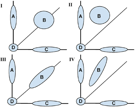
Figure 1. Conceptual diagram for fMRI activation distributions based on the motivating study of motor learning. Shaded areas represent learning based (inter-session differences) between a trained (Y axis) and untrained (X axis) task. Across all panels, Area (A) represents voxels with change in activation across sessions only in the trained task, (B) represents voxels with change in activation across sessions in both the trained and untrained task, (C) voxels with change in activation across sessions only in the untrained task, (D) represents no change in activation for both tasks. The four panels (I–IV) represent different potential shapes of the activation distributions for (B) with (I, II) showing a two dimensional shape and (III, IV) showing an approximately one dimensional. In (I, III) inter-sessions differences are symmetrically represented whereas in II, IV one task had a uniformly greater increase.
It is the shape of (B) that is of primary interest. For instance, any shift in B above the diagonal line represents training based learning. If the shape is spherical, there is no correlation between training status and change in activation across sessions. In contrast, the more ellipsoidal the shape, the greater the correlations in activation extent across sessions.
While acknowledging that SPM operates voxel-by-voxel, and that Figure 1 displays voxel groups, the SPM approach would investigate each point's distance from the diagonal line, assessing significance relative to inter-subject variability. Therefore, given enough data, the SPM approach would conceptually reject for voxels in groups (A) and (C) in the cases represented by all panels. However, it would reject most of the voxels in group B in panels II and IV only. The approach would reject few of the voxels in (B) for panels I and III. Contrast this with the shape and dimensionality of (B) being constant for panels I and II together and III and IV together. Thus, to the extent that learning represents itself as changes in the shape of the activation distribution, the voxel-wise approach would not tell the complete story.
Instead, we view the shape of the bivariate distributions of points in group (B) as informative for studying changes in task activation. One key attribute is its intrinsic dimensionality (1 vs. 2 dimensional). Ignoring groups (A), (C), and (D), one would conclude that (B) is two dimensional in panels I and II and intrinsically one dimensional in III and IV. The dimensionality of (B) is useful for differentiating whether changes in intensity or distribution account for activation changes following learning.
The use of principal components to investigate the dimensionality of learning builds upon an existing literature on the use of dimensionality testing in the study of activation maps (Worsley et al., 1997). Specifically, Zarahn (2002) and Moeller and Habeck (2006) considered it within the context of functional imaging. The aim of this work is to study the goals, limitations and hypotheses of tests of dimensionality of fMRI activation maps. A test of one vs. two dimensions on the set , that is rank(), investigates the null hypothesis
for unspecified c and collectively for all voxels v.
Let and recall that . Following the existing work on tests of dimensionality in fMRI, we use root tests of the second eigenvalue (see Mardia et al., 1980) to investigate the hypotheses of one dimension vs. two. A simulation-based investigation of this test follows. The simulation study includes: the strength of the effect, the intrinsic dimensionality (considering power and error rates), and the impact of biological and measurement variation, including variation in the angle of the subject-specific principal direction.
3. Materials and Simulation
3.1. Motivating Data Set
A motor learning study served as motivation for this work, though we emphasize that the methodology generally applies to any study of change in activation. The goal of the motor study centered on investigating skilled motor learning via the Arc Pointing Task (APT) (Shmuelof et al., 2012), where the task was designed to better understand neural correlates of motor skill acquisition. The subjects completed two similarly demanding motor tasks of drawing an arc within reference lines by moving their (non-dominant in all cases) left wrist. The interior circles in Figure 2 represent the starting and end points of the path. Subjects were directed to stay within the lines of the outer circles while tracing the arc. Subjects were scanned while performing the tasks at baseline and again 5 days later, with training on just one of the two tasks in the interim. Comparison of fMRI activation (or any measurement of motor function) from baseline to follow-up considers both effects related to motor learning and those related to changes between sessions. Comparison with the, otherwise similar, untrained task as a reference eliminates additive inter-session biases unrelated to learning.
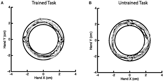
Figure 2. Example of the Arc Pointing Task (APT) executed within the fMRI session. Subjects were asked to navigate a cursor lying between the inner and outer concentric circles. Two tasks of similar difficulty were investigated. A horizontal task (A) where subjects were trained in between two scanning sessions and a vertical task (B) where subjects were not trained.
The specifics of the study are as follows. Thirteen right-handed subjects (8 females, 18–27 years of age) engaged in the above described motor tasks, none having performed these tasks previously. Subjects participated in a 5 day protocol consisting of daily behavioral sessions in the lab and two fMRI scans on the baseline and final days (1 and 5, respectively). During scanning, subjects performed the APT. Horizontal (trained) and vertical (untrained, control) APT movements were performed in separate block design experiments before and after training for the horizontal task. Six movements were performed in 18 blocks (repeated 6 times), at a slow speed (1.5 s per movement). Subjects received online feedback regarding the position of the cursor, but no further information about their success or failure, or about their movement speed. In the trained task, targets were presented on the horizontal line (same configuration as during the behavioral task in the lab) and in the untrained task, targets were aligned vertically. Movements were always in the clockwise direction. Subjects performed the movements with their (non-dominant) left wrist, while lying on their back, and receiving visual feedback of their movements through goggles (resonance technology, Los Angeles, CA). Further details on the experimental paradigm can be found in Shmuelof et al. (2014).
Data was acquired on a Philips Intera 3T scanner using a Philips SENSE head coil. The functional scans were collected using a gradient echo EPI, with voxel size of 3 × 3 × 3 mm (240 × 240 × 240 mm matrix). TR = 2 s, flip angle = 77o, axial slices, TE = 25 ms. Forty slices were gathered in an interleaved sequence at a thickness of 3 mm (no gap). Ninety − six volumes were accumulated in each experimental run. The first 2 volumes were discarded to allow magnetization to reach equilibrium. A single T1-weighted anatomical scan was also obtained for each subject (MPRAGE, 1 mm3).
Functional data were preprocessed using SPM5 (http://www.fil.ion.ucl.ac.uk/spm/software/spm5/). Before statistical analysis, the data was also corrected for slice timing acquisition and head motions, re-sliced to 2 × 2 × 2 mm voxels using a fourth degree B-spline interpolation, and transformed into a Talairach standard space (Talairach and Tournoux, 1988). A general linear model was used for data analysis, followed by calculation of beta maps. Scatter plots of beta before training and after training are shown in Figures 3, 4.
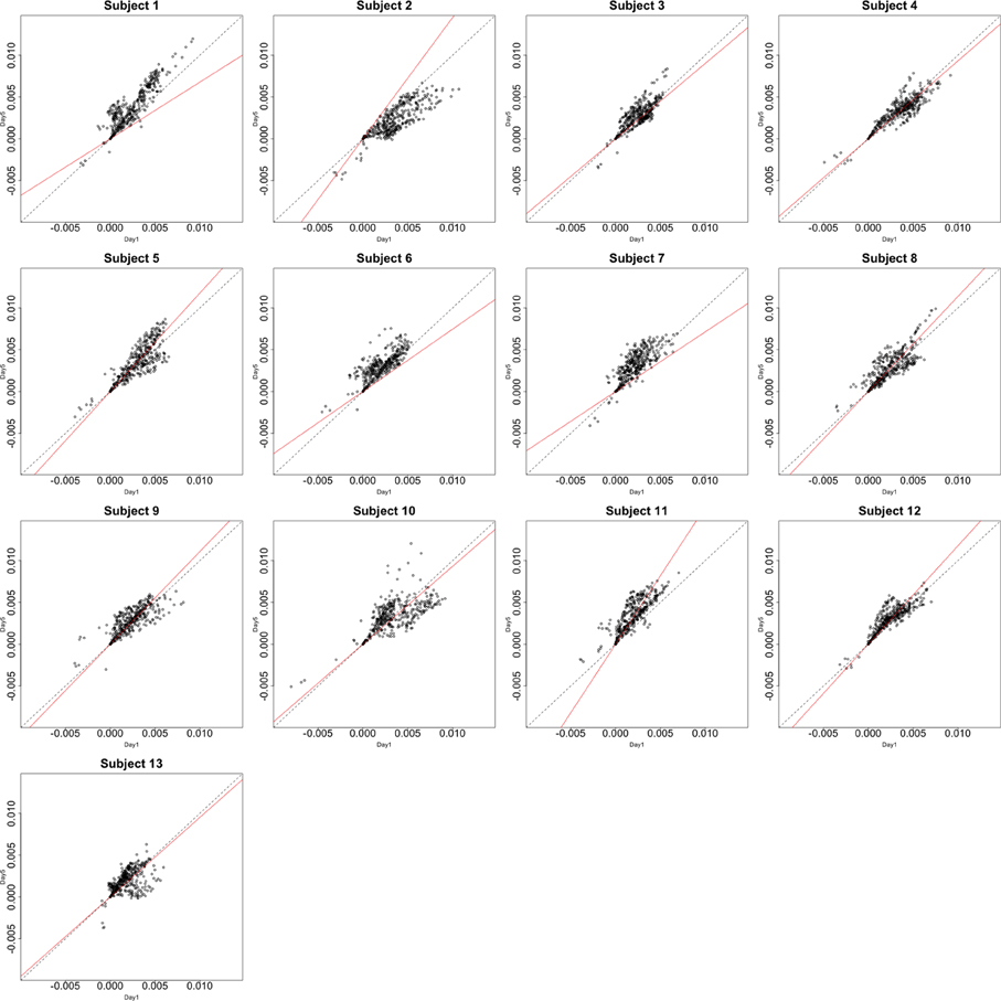
Figure 3. Contrast maps from the horizontal arc pointing task. The X axis for each plot is the first session while the Y axis is the second. Red lines show the direction of the first principal component while a dotted identity line is shown for reference.
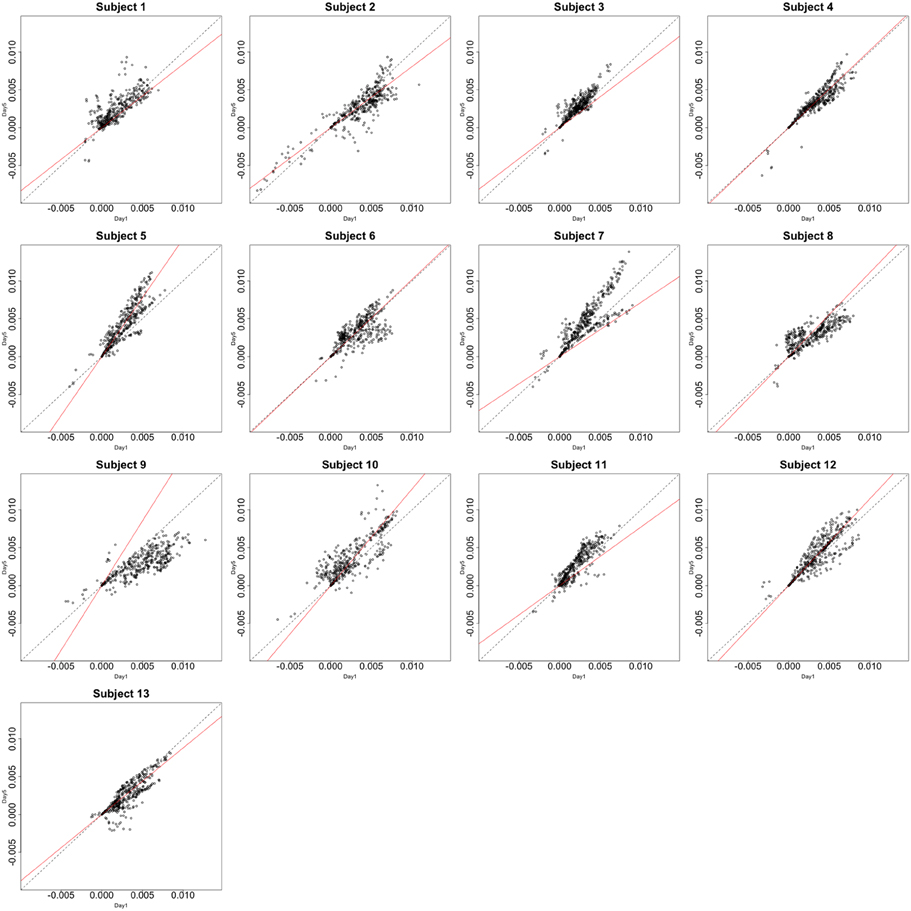
Figure 4. Contrast maps of the vertical arc pointing task. The X axis for each plot is the first session while the Y axis is the second. Red lines shows the direction of the first principal while a dotted identity line is shown for reference.
By comparing the trained and untrained tasks, the population impact of learning was estimated by considering differences in the change in activation maps over sessions. Using the developed notation, the collections compared are, {β21(v) − β11(v)}v = 1, … V to {β22(v) − β12(v)}v = 1, …, V, where, as previously noted, the first index indicates session (baseline and fifth day) and the second indicates task (horizontal and vertical). The test of dimensionality then considers whether the changes in activated voxels after training is uncorrrelated with the changes in the untrained (but otherwise similar) task. Under Gaussian assumptions, absence of correlation among activated voxels implies that the extent of activation is unrelated between sessions.
All subjects gave written, informed consent and received a small compensation for participating in the Study, which was approved by the Columbia University Institutional Review Board.
3.2. Simulation Study
Assume there are V = V1 + V2 voxels in total: V1 that are significantly different across sessions (group B in Figure 1) and referred to as “activated,” and V2 that are not (group D in Figure 1). Under this working example, the term activated implies a non-zero change in the contrast values across sessions. Thus, is the percentage of non-activated voxels.
The simulation model is:
where δ(v) = {δ1(v), δ2(v)} = {β21(v) − β11(v), β22(v) − β12(v)} and biv = {b1iv, b2iv} is a subject-specific realization plus noise. The generation of the δ(v) parameters varied across simulation settings, and is described separately for each case below.
In all simulation settings, the estimate of the V × 2 matrix of the δ(v), labeled , was obtained via the voxel-specific mean across subjects. Following Worsley et al. (1997), the V × 2 matrix, Z, denotes divided by its standard error. That is, make up row v and column k of Z. Here the variance was calculated across subjects separately for each voxel. The cross-product matrix is then
The Lawley/Hotelling trace statistic is:
where λj, j = 1, 2, …, h are the eigenvalues of S, h is the total number of eigenvectors and q is the testing rank. Under independence and Gaussian assumptions, Sq follows an F distribution under the null hypothesis, where the first q principal components capture all of the signal. In our case, h = 2, q = 1 and the test statistic is simply the second eigenvalue of S.
3.2.1. Simulation Under the Null Hypothesis
The first simulation setting considers the hypothesis of unidimensionality; that is, whether δ1(v) = cδ2(v), where c is constant across subjects. The parameter δ1(v) for the activated voxels was simulated as uniformly distributed in [min, max], with this range computed from values of [0, 1]–[10, 15]. Note that for voxels inactive in both time points, δ1(v) = 0. Thus, δ1(1), …, δ1(V1) ≠ 0 while δ1(V1 + 1), …, δ1(V) = 0. Note that, δ2(v) = cδ1(v) regardless of null status.
Figure 5 shows example data for a simulated subject as well as the estimated statistics. The null simulation varied according to the following: (i) distance of the activated voxels from the inactivated ones, as well as the range of activation, (controlled by min and max); (ii) the percentage of inactivated voxels (π); and (iii) the number of subjects (N). For all of the null hypothesis scenarios, c = 1. The type I error rates correspond to the percentage of rejections of the Lawley/Hotelling trace statistic for each simulation setting. The specifics of each scenario are described below while the results are shown in Table 1.
Simulation under variation in the distance: In this scenario, N = 12, V1 = 40, V2 = 200, and σ = 1. Five scenarios for each pair of min and max were considered. The results suggest that the type I error is not significantly affected by the distance of the activated voxels from the inactivated ones.
Changing the percentage of inactivated voxels: In this case, N = 12, σ = 1, min = 0.5, and max = 1.5. The total number of voxels was set at V = 240. These results suggest that the test is not significantly affected by the percentage of inactivated voxels.
Varying the number of subjects: In this case, V1 = 40, V2 = 200, σ = 1, and [min, max] = [0.5, 1.5]. The results imply that the type I error does not change significantly as N varies.
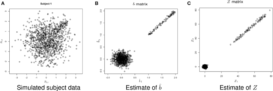
Figure 5. Example simulated data. (A) Shows the simulated data. (B) Shows the estimate of b using Equation (1). (C) Shows the estimate of Z, where .

Table 1. Results of the simulation studies.
3.2.2. Simulation Under the Alternative Hypothesis
There are a variety of ways in which the null hypothesis can fail to be true; herein, several key departures were analyzed. First, consider a straightforward departure, where Figure 1 holds, with sets (A) and (C) both empty. The extent of spherical and elliptical variation around the principal axis are evaluated. However, other departures could also be present. Most importantly, the null could be true for each subject, but with a varying angle along the principal axis. In addition, a non-trivial percentage of voxels changing activation status (i.e., sets (A) and (C) from Figure 1 being non-empty) would similarly represent a departure from the null hypothesis. The simulation scenarios for these parameters are described below.
The number of subjects remains N = 12 while min = 0.5, max = 1.5, V1 = 40, and V2 = 200.
Simulation under a basic alternatives: Two basic alternative settings were considered. In the first, the δ(v) were simulated as two dimensional, yet one dimension dominates the other. This method of simulation added orthogonal variation around the line used in the simulation under the null hypothesis. Specifically, the activated voxels have Gaussian variation orthogonal to the major axis (see Figure 6A). This was done in lieu of simulating a bivariate Gaussian with a non-zero correlation to consider an even, non-concentrated spread along the major axis. Simulations using a bivariate normal yielded similar results. In the second setting the correlation was assumed to be zero (see Figure 6B).
Variability of the angle of the principal axis Consider a null setting, as in Section 3.2.1. However, assume that the constant, c, varies across subjects. Let ci denote this constant for subject i. To simulate the data, first the null simulation from Section 3.2.1 was performed then the observed bivariate points {b1iv, b2iv} were multiplied by the rotation where θi is a subject-specific rotation angle from the 45o line, generated from a Gaussian distribution with mean 0 and standard deviation σa, which varied from 0.01 to 0.5. Before the rotation, c = 1, while afterwards, ci = tan (45o − θi). Examples of the simulated data are shown in Figure 7.
Changing Activation Sets In this setting, the impact of a non-trivial percentage of voxels, or change in voxels that switch activation status, i.e., corresponding to a large collection of voxels in sets (A) and (C) in Figure 1. An example simulation is shown in Figure 8. Here, the bkiv were either 0 or uniform, where a min = 0.5 and max = 1.5. The specific values were: 200 voxels set to be inactive for both the trained and untrained tasks, 40 voxels set to be activated for the trained and untrained groups, Va voxels were activated with training, but inactivated without training, while another Va voxels were inactivated with training but activated without training. Here Va was varied between 10 and 400. Note that, in this setting, the Z matrix (see Figure 8) is substantially different from the direction of its first eigenvector.
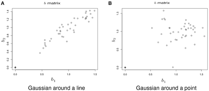
Figure 6. Example simulation from the alternative hypothesis. The axes are the two dimensional bivariate simulated data representing inter-session differences for each task in the motivating study. In (A) the voxels have Gaussian variation added orthogonally to the major axis. In (B) there is no relationship.
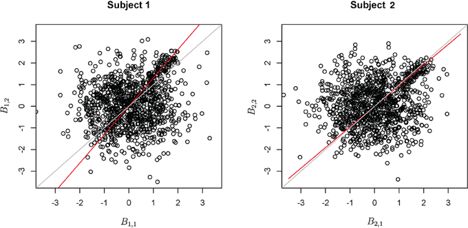
Figure 7. Example simulation for the setting when the principal axis differs across subjects. The axes are the two dimensional bivariate simulated data representing inter-session differences for each task in the motivating study. The gray line is a reference identity line, while the red line is the axis of principal direction.
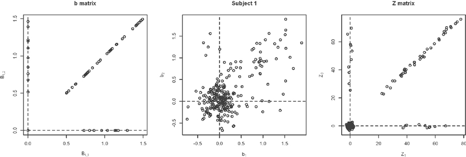
Figure 8. Example simulation from the alternative with changing activation sets. The axes are the two dimensional bivariate simulated data representing inter-session differences for each task in the motor learning study. Shown are the true parameter values (leftmost panel), the simulated subject data (middle panel) and the Z-values (rightmost panel).
3.3. Simulation Results
Table 1 displays the results across the simulation settings. All tests were performed at a nominal 5% error rate.
3.3.1. Simulations Under the Null Hypothesis
Adherence to the specified nominal error rate was remarkably consistent as parameter settings varied. When varying the distance, the test showed only slight liberalism (Type I error rate larger than the nominal) across settings. Only for unrealistically small activation sets did the test demonstrate liberalism when altering the activation set size. In addition, varying the number of subjects had little impact. Adherence to the nominal error rate was acceptable, even at very low numbers of subjects.
3.3.2. Simulations Under the Alternative Hypothesis
Under the basic alternative, where the true voxel states possessed a strong (but not perfectly linear) corelation, power varied as expected. Under a strong correlation (σb close to 0), power trended to the nominal type I error rate. Encouragingly, power quickly trended to one as the true relationship moved away from a dominant dimension. As expected, the power tended to 1 as the sample size increased (confirming the relevant asymptotics). However, the sample size needed to be relatively large to have adequate power at the modest value of σb = 0.2.
In the case where no dimension dominated under the basic alternative of absence of correlation, power changed significantly with the spread of activation, σb. When the angle of principal direction varied, power suffered dramatically. To address this, a first stage subject-specific principal components rotation was investigated. This appeared to improve power in settings where the null and non-null voxels were more clearly delineated, but continued to exhibit low power (11%) when the distance was large (min = 10, max = 15). A non-trivial fraction of voxels changing activation status had a negative impact on power.
4. Data Analysis of the Motivating Data Set
This section investigates the impact of training on activation using the APT data described in Section 3.1 and represented in Figures 3, 4, which show estimated beta maps. A null hypotheses suggests that the data points are close to the principal line. Notably, a distinction between the null and alternative hypothesis is difficult to ascertain graphically. However, it is apparent that the axis of principal direction varies by subject. Next, dimensionality is tested via three methods: first considering only the (trained) horizontal task, then only the (untrained) vertical task, and then comparing both. When considering the untrained task in isolation we are testing H0: β21(v) = cβ11(v), then H0:β22(v) = cβ12(v) for the trained and H0: β21(v) − β11(v) = c{β22(v) − β12(v)} when comparing trained and untrained. (The paper used the latter as the primary motivating example.) In Table 2, the results before and after angle correction are shown.
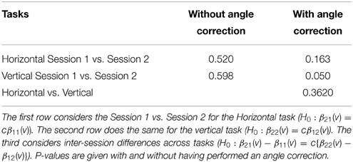
Table 2. P-values of the tests of dimensionality for the motor learning data set.
4.1. Motor Learning Data Results
The axis of principal direction varied by subject (see Figures 3, 4). Before correcting for the principal angle, the tests of dimensionality were insignificant, for both the horizontal and the vertical tasks. However, after correcting the principal angle by subject, the p-values of the tests were highly reduced. Focusing only on the tasks separately, the test of dimensionality yielded a p-value of 0.05 for the vertical task and 0.16 for the horizontal one. When comparing across tasks, the p-value was 0.36. Thus, the untrained task has a significant second dimension that does not appear to be present in the trained. Inspecting the data, excess variability in the trained task appears to be due to biomodal changes in activation. It is not surprising that the comparison across tasks was non-significant, given the increased variability obtained from taking differences and the issues of power for the test.
5. Discussion
5.1. Simulation Results
The simulation results suggest that tests of dimensionality are a reasonable exploratory testing procedure for investigating the distribution of paired activation maps. However, their confirmatory performance was hindered by instances with low power in situations that could be realistically seen in practice. The adherence to the nominal type I error rate, on the other hand, was uniformly acceptable across simulation settings. Thus, a rejection from this test is likely informative, while an acceptance less so.
The low power cases occurred where there is substantial variability in the principal axis, or where activation status changed. This latter condition created confusion between noise and signal, with the test attributing signal variability as noise. Of the two cases, careful masking could eliminate concern over changing activation status. However, variability in the principal axis is likely the norm and could arise from a number of plausible biological, technological and processing causes. The straightforward refinement of a first stage subject-level principal component rotation improves the power.
5.2. General Discussion
This manuscript posited a different paradigm for statistically evaluating learning using task-related BOLD fMRI activation maps. At its core, the primary advance is the supposition of using the bivariate distribution of the activation maps, or changes in activation maps, when comparing tasks over sessions. Under this framework, changes in the distribution of activated voxels are key, not voxel level changes in activation extent, as would be evaluated in voxel-level parametric mapping interaction tests. An unintended benefit of this distributional approach in this setting is avoiding the familiar issue of having to determine interactions where main effects are not present.
The intended benefit of increasing power over voxel-level interaction tests was found to be true, provided assumptions hold. For example, Figure 9 provides a simulation example where the alternative test of dimensionality is both true and detected (P-value of 0.03). However, only 11% of the voxels would satisfy a voxel level test of significance. We emphasize the different nature of the hypotheses interrogated by these approaches so that comparisons of power should be taken with a grain of salt.
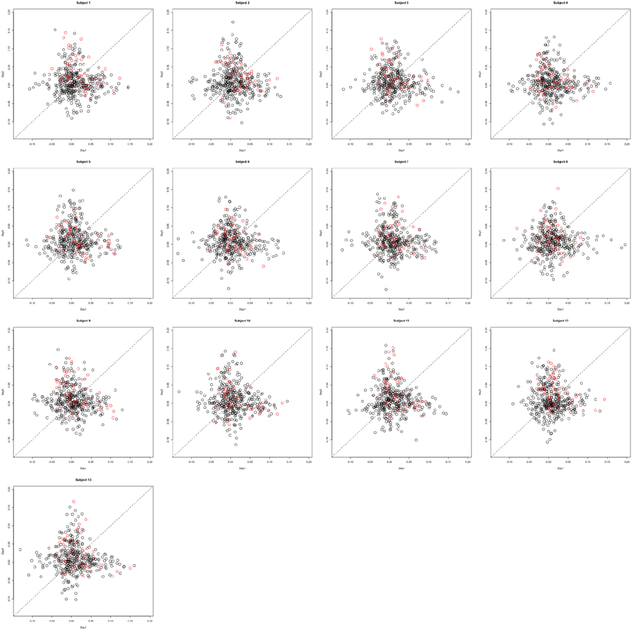
Figure 9. A simulation example highlighting increased power for detecting learning based differences. The axes are the two dimensional bivariate simulated data representing inter-session differences for each task in the motivating study. The alternative of the dimensionality test is true and the P-value is 0.03, suggesting that activation extent is unrelated between tasks. However, only 11% of the voxels satisfy a voxel level test of significance (colored in red).
Evaluating distributional differences for learning-based activation tests a different scientific hypothesis than voxel level testing. In our example, the question was how BOLD activation, or changes in activation, relate between trained and untrained tasks. Investigating activation distributions is less sensitive to the requirement of focal localization of effects compared to interaction testing. For example, two small spatially separated significant interaction regions may have different voxel-level interaction significance than a single contiguous region of the same aggregate size. In contrast, the distribution may not change. Conversely, evaluating contrast map distributions does not provide the benefits of localization to inform results.
It is worth emphasizing that the investigation of activation distribution represents a complementary procedure to voxel-level testing and does not represent a form of omnibus test to be performed prior to it. Thus, it is perhaps not useful to generate a single analytic pipeline, whereby omnibus distributional tests are followed by voxel level contrasts of interest.
An interesting next direction in this line of research would consider full models of the joint distribution of {β11(v), β12(v), β21(v), β22(v)}. This could be accomplished using a Bayesian random effects approach via mixtures of Gaussian random variables. However, the feasibility, applicability and gain of such an approach over simpler solutions remains unknown. A tantalizing possible benefit would be robustness to inter-subject registration to a template. In contrast, interaction tests focus on localization and as such, place a heavy burden on accurate inter-subject registration. A full random effect mixture model could possibly remove the need for inter-subject registration, or at least remove the need for non-affine registration.
The far simpler approach discussed in this manuscript addresses dimensionality. The results show that the operating characteristics of the approach are viable, if modeling assumptions are met. Particularly encouraging was the robustness to variation in the distance of the center of activation from null voxels. However, its sensitivity to the angle of the principal axis is a core issue, as such variation is clear from the data.
In the real data analysis it is noteworthy that the vertical and horizontal tasks differed in their respective tests of dimensionality. Particularly, the null hypothesis was not rejected in the trained task (horizontal) while it was in the untrained task (vertical). However, there does appear to be more apparent non-Gaussianity in the vertical task, suggesting a component of the rejection is related to a form of dimensionality not well-covered by the model. The contrast test comparing vertical vs. horizontal was not significant. Therefore, it cannot be concluded that the activation distribution given by the inter-session differences across tasks is not linear. For all three cases, the data analysis suggests large variability in the subject-specific principal axes, a setting where low power was evidenced in the simulation study. Thus, the null results are perhaps indicative of low power.
Conflict of Interest Statement
The authors declare that the research was conducted in the absence of any commercial or financial relationships that could be construed as a potential conflict of interest.
References
Diggle, P., Heagerty, P., Liang, K., and Zeger, S. (2002). Analysis of Longitudinal Data, Vol. 25. Oxford: Oxford University Press.
Friston, K., Ashburner, J., Kiebel, S., Nichols, T., and Penny, W. (2011). Statistical Parametric Mapping: The Analysis of Functional Brain Images: The Analysis of Functional Brain Images. London: Academic Press.
Lindquist, M. (2008). The statistical analysis of fmri data. Stat. Sci. 23, 439–464. doi: 10.1214/09-STS282
Lindquist, M., Meng Loh, J., Atlas, L., and Wager, T. (2009). Modeling the hemodynamic response function in fmri: efficiency, bias and mis-modeling. Neuroimage 45, S187–S198. doi: 10.1016/j.neuroimage.2008.10.065
PubMed Abstract | Full Text | CrossRef Full Text | Google Scholar
McLachlan, G., and Peel, D. (2000). Finite Mixture Models, Vol. 299. New York, NY: Wiley-Interscience.
Moeller, J., and Habeck, C. (2006). Reciprocal benefits of mass-univariate and multivariate modeling in brain mapping: applications to event-related functional mri, h 2 15 o-, and fdg-pet. Int. J. Biomed. Imaging 2006:79862. doi: 10.1155/IJBI/2006/79862
PubMed Abstract | Full Text | CrossRef Full Text | Google Scholar
Nichols, T., and Holmes, A. (2001). Nonparametric permutation tests for functional neuroimaging: a primer with examples. Hum. Brain Mapp. 15, 1–25. doi: 10.1002/hbm.1058
PubMed Abstract | Full Text | CrossRef Full Text | Google Scholar
Shmuelof, L., Krakauer, J. W., and Mazzoni, P. (2012). How is a motor skill learned? change and invariance at the levels of task success and trajectory control. J. Neurophysiol. 108, 578–594. doi: 10.1152/jn.00856.2011
PubMed Abstract | Full Text | CrossRef Full Text | Google Scholar
Shmuelof, L., Yang, J., Caffo, B., Mazzoni, P., and Krakauer, J. W. (2014). The neural correlates of learned motor acuity. J. Neurophysiol. 112, 971–980. doi: 10.1152/jn.00897.2013
PubMed Abstract | Full Text | CrossRef Full Text | Google Scholar
Talairach, J., and Tournoux, P. (1988). Co-Planar Stereotaxic Atlas of the Human Brain. 3-Dimensional Proportional System: an Approach to Cerebral Imaging. New York, NY: Thieme.
Worsley, K., Poline, J., Friston, K., and Evans, A. (1997). Characterizing the response of pet and fmri data using multivariate linear models. Neuroimage 6, 305–319. doi: 10.1006/nimg.1997.0294
PubMed Abstract | Full Text | CrossRef Full Text | Google Scholar
Zarahn, E. (2002). Using larger dimensional signal subspaces to increase sensitivity in fmri time series analyses. Hum. Brain Mapp. 17, 13–16. doi: 10.1002/hbm.10036
PubMed Abstract | Full Text | CrossRef Full Text | Google Scholar
Keywords: canonical variates analysis, cognitive learning, BOLD fMRI, statistical parametric mapping, interaction test
Citation: Yang J, Shmuelof L, Xiao L, Krakauer JW and Caffo B (2015) On tests of activation map dimensionality for fMRI-based studies of learning. Front. Neurosci. 9:85. doi: 10.3389/fnins.2015.00085
Received: 13 December 2013; Accepted: 26 February 2015;
Published: 14 April 2015.
Edited by:
Russell A. Poldrack, University of Texas, USAReviewed by:
Lei Wang, Northwestern University Feinberg School of Medicine, USAAnand Joshi, University of Southern California, USA
Christopher W. Tyler, Smith-Kettlewell Eye Research Institute, USA
Copyright © 2015 Yang, Shmuelof, Xiao, Krakauer and Caffo. This is an open-access article distributed under the terms of the Creative Commons Attribution License (CC BY). The use, distribution or reproduction in other forums is permitted, provided the original author(s) or licensor are credited and that the original publication in this journal is cited, in accordance with accepted academic practice. No use, distribution or reproduction is permitted which does not comply with these terms.
*Correspondence: Juemin Yang, Department of Biostatistics, Johns Hopkins Bloomberg School of Public Health, 615 N Wolfe Street Baltimore, MD 21205, USA juyang@jhsph.edu