Bayesian Tractography Using Geometric Shape Priors

The problem of estimating neuronal fiber tracts connecting different brain regions is important for various types of brain studies, including understanding brain functionality and diagnosing cognitive impairments. The popular techniques for tractography are mostly sequential—tracts are grown sequentially following principal directions of local water diffusion profiles. Despite several advancements on this basic idea, the solutions easily get stuck in local solutions, and can't incorporate global shape information. We present a global approach where fiber tracts between regions of interest are initialized and updated via deformations based on gradients of a posterior energy. This energy has contributions from diffusion data, global shape models, and roughness penalty. The resulting tracts are relatively immune to issues such as tensor noise and fiber crossings, and achieve more interpretable tractography results. We demonstrate this framework using both simulated and real dMRI and HARDI data.

1. Introduction

This paper considers an important problem of estimating major white matter fiber tracts in human brain using diffusion magnetic resonance imaging (dMRI) images (Mori et al., 2005). The construction of fiber tracts connecting different brain regions is an important first step toward studying brain connectomics and its implications in assessment of brain functionality, including cognitive abilities and general health. Spurred by experimental development of large databases involving human subjects, with samples across different demographic groups, there is a emerging interest in representing and quantifying brain connectivity patterns. Therefore, efficient and reliable fiber tracking algorithms are urgently needed. However, the problem of estimating fiber tracts using dMRI data is far from being solved (Maier-Hein et al., 2016). The current solutions have many limitations, including inefficiency and susceptibility to noisy, corrupt, and low-quality data. The data mostly comes from pre-processed dMRI images, providing at each voxel a measure of diffusivity of water molecule at that location. The representation of this diffusivity is generally a 3 × 3 symmetric, positive definite matrix (SPDM), also called a tensor. In situations where higher resolution data are available, one constructs high angular resolution diffusion imaging (HARDI) data; at each spatial location the orientation diffusion function (ODF, a function on a unit sphere §²) is estimated (Descoteaux, 2015). Given these local diffusivity measures, one seeks to form fiber tracts, or their collections in the form of fiber bundles, between regions of interest (ROIs), and to further develops structural networks (Cheng et al., 2012; de Reus and van den Heuvel, 2013; Fornito et al., 2013; Durante and Dunson, 2017). This paper focuses on estimation of fiber tracts, also termed tractography, using dMRI and HARDI data. For any two regions (voxels) in a brain coordinate system, the goal is to estimate a collection of curves that follow an optimal pattern of fluid flow connecting these locations, while conforming to anatomical reasonings and interpretations.

Due to the importance of tract-based connectivity in brain connectomic analysis, there have been a number of solutions developed for estimating fiber tracts. They can be loosely grouped into two categories: local and global methods. Local methods construct fiber curves sequentially based on the estimated local diffusion directions. Depending on the mechanism for specifying a local propagation direction, one can further classify the local methods into deterministic methods (Mori et al., 1999; Basser et al., 2000) or probabilistic methods (Hagmann et al., 2003). While the deterministic methods mainly follow the local principal directions to grow fiber curves, the probabilistic methods propose a propagation direction from voxelwise probability distribution, e.g., orientation distribution function (ODF), for growing fibers. The first successful deterministic tractography algorithm was dubbed FACT (fiber assignment by continuous tracking), which has been widely studied in the literature (Mori and van Zijl, 2002). But the limitations of FACT and similar methods are obvious. They include sensitivity to initialization, the susceptibility of principal direction estimation to local noise, and lack of connectivity information between regions of the brain. These limitations drive people to use the probabilistic algorithms. One advantage of the probabilistic methods is that they are based on the full, albeit local, distribution of fiber directions, rather than just the principal direction. They can output a connectivity index measure, e.g., the number of fiber curves, between any two regions of interest, indicating the probability with which the regions are connected to one another. However, this creates problems when the local diffusion directions are not well estimated or are overly smooth. On the other hand, the global methods try to reconstruct fiber curves simultaneously by optimizing the configuration that best matches the given data. Finding the fiber curves that best matches the given data is a hard inverse problem. Current solutions are to translate this inverse problem into a forward problem using a Bayesian approach. For example, Reisert et al. (2011) used a Metropolis Hastings sampler to propose small line segments to fit the given dMRI data and use them to further generate long fiber curves. The global methods provide a better stability with respect to the noise and imaging artifacts. However, there are some issues with the current global methods also. The Bayesian methods typically have high computational cost and require huge memory space, to compute and store a whole ensemble of solutions. Also, in an optimization setting, it is difficult to avoid local solutions since no additional structure is imposed on the optimization.

We can summarize the limitations of current methods as follows: (a) The local methods are essentially sequential—they start fibers from one end and grow them over time. This one-boundary solution is not natural for tractography, which is actually a two-boundary problem. (b) The local tractography algorithms are highly susceptible to fiber crossing, noise and imaging artifacts. Incorrect recording or noisy observations of tensors can send algorithms in wrong directions and it is difficult to recover from such misdirections. (c) The global tractography algorithms achieve better stability with respect to noise, but they are very computationally expensive. (d) Both local and global methods tend to produce a large proportion of false positive fibers because of the noise and ambiguity at fiber crossings. Figure 1 shows some examples of limitations of a local streamline method, where the blue lines denote ground truth, the red and green lines are tractorgraphy results from the classic FACT method. The left panel shows the challenge of fiber crossing, where the sequential approach fails to reach the target region. The right panel shows the effect of having a patch of noisy data in the middle. The fibers from either regions run into this noisy patch and fail to reach the other end. Additional examples of the challenges faced by streamline methods on the real data, are shown later in the experimental results section. A global approach used for estimating fiber tracts, or curves in general image data, is called active contours, where one evolves a curve in order to minimize an energy functional (Pichon et al., 2005; Lankton et al., 2008; Melonakos et al., 2008; Eckstein et al., 2009; Mohan et al., 2009; Zach et al., 2009; Li and Hu, 2013). Other global techniques (Faugeras et al., 2004), including a variation of Kalman Filter (Cheng et al., 2015), have also been applied to this problem.

FIGURE 1

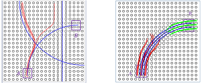
Figure 1. Two examples of the classic streamline method does not work. The blue lines are ground truth fibers. The red and green lines are the tractorgraphy results from the FACT method. Starting from area A, FACT failed to reconstruct the fiber tracts that connect A and B.

In this paper, we propose a new approach that is essentially a global method but using additional geometry information for ensuring optimal solutions. The proposed method is fast and easy to implement, and robust to the noise in the data. Most importantly, it can incorporate the prior knowledge from anatomical structure and brain connectomics. Rather than growing fiber tracts sequentially, our idea is to initialize fiber tracts between regions of interest as Euclidean curves and then deform them iteratively using gradients of a posterior energy. This approach, termed Bayesian Active Contours (Joshi and Srivastava, 2009; Bryner et al., 2013), estimates fiber tracts under an energy function that has contributions from three sources: the given data or the likelihood term, the prior knowledge on the geometric shapes of fibers connecting these ROIs, and a roughness penalty. The algorithm uses the gradient of this posterior energy to iteratively update curves into high probability and highly interpretable fiber tracts. The prior on the geometric shapes relies on developing statistical shape models of fiber curves between ROIs, using atlas data, and evaluating expressions for gradient of resulting shape model energy with respect to the shape variable. We use advances in elastic shape analysis of Euclidean curves to develop efficient statistical models for fiber bundles using training (or atlas) data. The training data can be generated using existing local or global tractography algorithms, or can use manual inputs. These models form prior information for future tractography and, in conjunction with diffusion data likelihood, they provide tract estimation results.

In contrast to the probabilistic tractography method (Behrens et al., 2003, 2007), the proposed Bayesian method is a global one. We start with an initial fiber connecting two pre-specified regions and update it under an energy function. The final fiber can best explain the diffusion data under the constraints of prior shape distribution and desired smoothness. Previously, there are some Bayesian tractography methods proposed in the literature (Friman et al., 2006; Cook et al., 2008; Yap et al., 2011). These methods are different from the proposed one: in our method, we assign a prior on the fiber shape space, while in (Friman et al., 2006; Cook et al., 2008; Yap et al., 2011), the prior is imposed on local fiber orientation distribution. Probably, the most similar work to ours is (Christiaens et al., 2014), where an atlas-guided global tractography is introduced with a prior on the local tract distribution. However, our work is different in two aspects: Firstly, we have a different energy function. We introduce a novel data term and a smoothness term separately to measure alignment between fibers and diffusion data, and the smoothness of fiber tracts. Secondly, we have a different prior. We incorporate the prior information of fiber shape from the atlas space while (Christiaens et al., 2014) obtains the prior information of local tract distribution from the atlas space.

The rest of this paper is organized as follows. We describe the three components of the posterior energy—data likelihood, shape prior and roughness penalty—and their gradients in Section 2. The resulting tractography algorithm is laid out in Section 3, and experimental results using both simulated and real data, the extension to HARDI data are presented in Section 4. We close the paper with a short discussion in Section 5.

2. Mathematical Framework for Bayesian Tractography

Although the framework can be easily generalized to 3D data, we will restrict to 2D data in this paper for simplicity. The theory is general enough to be applicable to 3D data directly.

First, we develop a mathematical framework for estimation of fiber tracts using tensor data and prior shape models. Let ${P}$ be the set of 2 × 2 symmetric, positive definite matrices (or tensors). For the domain, D = [0, 1]², let M : D → ${P}$ denote a continuous vector field of tensors defined on this domain. Let β:[0, 1] → D be an absolutely continuous curve contained in this domain, and let ${B}$ be the set of all such curves. Our goal is to find a β with certain boundary constraints that optimizes a chosen objective function that comes from a Bayesian formulation. Thus, we pose the problem of tractography as a MAP estimation. In this formulation we seek parameterized curve $\widehat{\beta }$ that minimizes an energy functional according to: $\widehat{\beta }={\mathrm{\text{argmin}}}_{\beta \in {B}}{E}_{total}(\beta )$, where

$\begin{array}{ll}{E}_{total}(\beta )={\lambda }_1{E}_{data}(\beta )+{\lambda }_2{E}_{prior}(\beta )+{\lambda }_3{E}_{smooth}(\beta ).& (1)\end{array}$

This total energy functional has contributions from three different criteria that are weighted by the coefficients λ₁, λ₂, λ₃ > 0. The data energy E_data is defined solely from the diffusion data in the image, E_prior is the prior shape energy defined from a statistical model on shapes of the fiber β, and the smoothing energy E_smooth is a penalty that ensures a certain amount of smoothness in the estimated fiber. In order to minimize E_total we use a gradient descent procedure that updates the curve according to β ↦ β − δ∇_βE, where

$\begin{array}{ll}{\nabla }_{\beta }E={\lambda }_1\nabla E_{data}(\beta )+{\lambda }_2\nabla E_{prior}(\beta )+{\lambda }_3\nabla E_{smooth}(\beta ).& (2)\end{array}$

That is, we search for a local minimization of Equation (1) via gradient descent. The weights λ_i will certainly affect curve evolution, i.e., a large penalty on the smoothness term favors shorter fibers and so on. Through trial and error, one can adjust the λ's depending on the data and problem context. In the next three sections, we summarize the formulation of each of the three energy terms.

2.1. Data-Likelihood Term

The data term is designed to quantify the agreement of the fiber directions with the diffusion tensor at that location. Let M be a given tensor field and β be a curve lying in the domain D, as shown in the left panel of Figure 2. The data energy term is then given by:

$\begin{array}{ll}{E}_{data}[\beta ]={\displaystyle {\int }_0^1{n}_{\beta }{\left(t\right)}^T}{M}_{\beta (t)}^{-1}{n}_{\beta }(t)dt,\text{ where }{n}_{\beta }(t)=\frac{\dot{\beta }(t)}{|\dot{\beta }(t)|}.\hfill & (3)\end{array}$

FIGURE 2

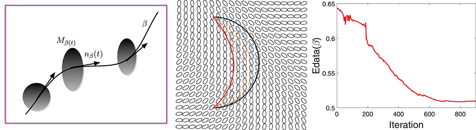
Figure 2. (Left) A schematic showing a curve β passing through a tensor field M. (Middle) An example of gradient-based optimization under E_data, where black is the initial curve and red is the final curve. (Right) The evolution of E_data during this optimization.

Here n_β(t) denotes the unit vector tangent to β at β(t) and M_β(t) is the tensor at location β(t) ∈ D. The integrand is lower at the locations where the fiber tract is aligned with the tensor field and vice-versa.

We motivate the choice of this expression by focusing on some Riemannian frameworks used in tractography:

• Maximal Curves Matching the Given Tensor Field: One generally wants to find curves such that their velocity vectors maximally match the given diffusion tensors. Therefore, one may consider maximizing the term:

$\begin{array}{l}{L}_M[\beta ]={\displaystyle {\int }_0^1\sqrt{(\dot{\beta }{(t)}^T{M}_{\beta (t)}\dot{\beta }(t))}}dt={\displaystyle {\int }_0^1|}\dot{\beta }(t){|}_{M_{\beta (t)}}dt.\end{array}$

This quantity is nothing but the length of a curve β in D under a Riemannian metric defined by the tensor field M. The maximizers of L_M are the longest paths between given points in D. However, the problem with this is that there is no upper bound on the length of the curve, and one can place arbitrarily long curves in D irrespective of M.

• Geodesics Under Inverse Tensor Field: A better idea is to use the inverse of the given tensor field at each point and then construct geodesic paths under that Riemannian metric (O'Donnell et al., 2002; Duncan et al., 2004; Melonakos, 2009), according to:

$\begin{array}{l}{\beta }^{\ast }={\text{argmin}}_{\beta }({\displaystyle {\int }_0^1\sqrt{(\dot{\beta }{(t)}^T{M}_{\beta (t)}^{-1}\dot{\beta }(t))}}dt\\ ={\displaystyle {\int }_0^1|}\dot{\beta }(t){|}_{M_{\beta (t)}^{-1}}dt).\end{array}$

One can solve the optimization problem by minimizing an energy, without the square-root in the integrand, as follows:

$\begin{array}{l}{\beta }^{\ast }={\text{argmin}}_{\beta }\left({\displaystyle {\int }_0^1\dot{\beta }}{(t)}^T{M}_{\beta (t)}^{-1}\dot{\beta }(t)dt\right).\end{array}$

This way one gets shortest curves such that their velocities agree with the dominant directions of the original tensor field. This formulation also agrees with a probabilistic approach where one uses the tensor field to define a Gaussian distribution at each point (Lenglet et al., 2004), and seeks maximum likelihood estimates. Although this method favors fiber directions similar to the dominant eigen vectors of the given tensor field, it additionally penalizes the lengths of the such fibers. Similar to the previous bullet, it may be possible to find shorter paths that do not agree with the tensor field. Some other papers (Fuster et al., 2014). Hao et al. (2014) have expressed this exact issue in different terms, citing the inability of this method to handle high curvature regions. They proposed a solution based on modifying the Riemannian metric by a curvature-based scalar field and then constructing geodesic paths (Hao et al., 2014). The real issue in these ideas is that there is no independent way to control the lengths of estimated fibers.

• Scale-Invariant Optimal Paths: We take a different approach where the length of the fibers is separated from the agreement of fiber directions with the given tensor directions. We weight these two quantities differently and are able to better control the length of the fibers. For the domain D, and a given tensor field M : D → ${P}$, we define an energy term given by

$\begin{array}{ll}{E}_{data}[\beta ]={\displaystyle {\int }_0^1{n}_{\beta }{\left(t\right)}^T}{M}_{\beta (t)}^{-1}{n}_{\beta }(t)dt,& (4)\end{array}$

where $n_{\beta }(t)=\dot{\beta }(t)/\left|\dot{\beta }(t)\right|$. Note that if we scale the speed of traversal along β by a constant, the energy function remains unchanged. In other words, the integrand only depends on the agreement of the direction n_β(t) with the dominant eigen vectors of M_β(t), and not on the speed of traversal at β(t). However, this energy function is not invariant to a re-parameterization of β. Let γ : [0, 1] → [0, 1] be a positive diffeomorphism, the β ◦ γ represents a re-parameterization of β. It can be seen that, in general, E_data[β] ≠ E_data[β ◦ γ]. If that invariance is desired, one can achieve it by changing the measure of integration from dt to $\left|\dot{\beta }(t)\right|dt$ in Equation (4).

The next step is to derive the gradient of E_data with respect to β for use in gradient-based optimization. To specify the gradient of E_data, we need some additional notation. Note that for any location x = (x₁, x₂) ∈ D, the gradient of M : D → ${P}$ has two components, ∇_x1M_x, ∇_x2M_x ∈ T_Mx(${P}$). Thus, the gradient vector ∇_xM_x is a higher-order tensor of the size 2 × 2 × 2. For any such tensor A ∈ ℝ^{2 × 2 × 2} and a vector x ∈ ℝ², we will use the notation: 〈〈A, x〉〉 to imply x₁A(:, :, 1)+x₂A(:, :, 2) ∈ T_M(x)(${P}$). Therefore, 〈(〈〈Ax〉〉)x〉 denotes a 2-vector given by $x_{1}A(:,:,1)x+x_{2}A(:,:,2)x\in {ℝ}^2$. With this notation, we can express the gradient of E_data as follows.

LEMMA 1. The gradient of E_data with respect to β, under the 𝕃² norm, is given by:

$\begin{array}{l}-2\{\frac{1}{|\dot{\beta }(t)|}\left(M_{\beta (t)}^{-1}{\dot{n}}_{\beta }(t)+\langle \langle {\nabla }_x{M}_{\beta (t)}^{-1},\dot{\beta }(t)\rangle \rangle n_{\beta }(t)\right)\\ -\frac{{\dot{\beta }}^T(t)\ddot{\beta }(t)}{|\dot{\beta }(t){|}^3}{M}_{\beta (t)}^{-1}{n}_{\beta }(t)-\frac{1}{|\dot{\beta }(t)|}({\dot{n}}_{\beta }(t)n_{\beta }^T(t)M_{\beta (t)}^{-1}{n}_{\beta }(t)\\ +n_{\beta }(t)n_{\beta }^T(t)\langle \langle {\nabla }_x{M}_{\beta (t)}^{-1},\dot{\beta }(t)\rangle \rangle n_{\beta }(t)+2n_{\beta }(t)n_{\beta }^T(t)M_{\beta (t)}^{-1}{\dot{n}}_{\beta }(t))\\ +\frac{{\dot{\beta }}^T(t)\ddot{\beta }(t)}{|\dot{\beta }(t){|}^3}{n}_{\beta }(t)n_{\beta }^T(t)M_{\beta (t)}^{-1}{n}_{\beta }(t)\}+\langle \langle tran({\nabla }_x{M}_{\beta (t)}^{-1}),n_{\beta }(t)\rangle \rangle n_{\beta }(t).& (5)\end{array}$

where $tran({\nabla }_x{M}_{\beta (t)}^{-1})$ is transpose of ${\nabla }_x{M}_{\beta (t)}^{-1}$.

A derivation of this expression is presented in the Appendix. Having an analytical expression for ∇_βE_data makes the optimization problem more efficient, as compared to purely numerical solutions.

Figure 2 shows an example of the gradient-based minimization of E_data in the middle panel. It shows a tensor field M and an initial curve β (in black). We update β iteratively using −∇_βE_data and the result is drawn as a red curve. The corresponding evolution of E_data is plotted in the right panel.

2.2. Smoothness or Fiber Length Term

For regulating smoothness of the estimated curve, we follow a common approach from geometric active contours that is motivated in part by Euclidean heat flow. Define the smoothing energy function as $E_{smooth}(\beta )={\int }_0^1\left|\dot{\beta }(t)\right|dt$, which is equal to the length of the curve and is naturally invariant to any re-parameterization. It is shown in Kichenassamy et al. (1995) that the gradient of E_smooth is given by the Euclidean heat flow equation ∇E_smooth(β) = κ_βn_β, where κ_β is the curvature at each point of β and n_β is the unit normal field along the curve. It is well known that this particular penalty on a curve's length leads to simultaneous smoothing and shrinking of a curve. If we rescale the curve to keep the original length, the main effect is that of smoothing. An example of this idea is illustrated in Figure 3 that shows a curve evolving according to −∇E_smooth. The left panel shows the initial curve (in black), and its updates using the negative gradient of E_smooth. The corresponding decrease in E_smooth is plotted on the right.

FIGURE 3

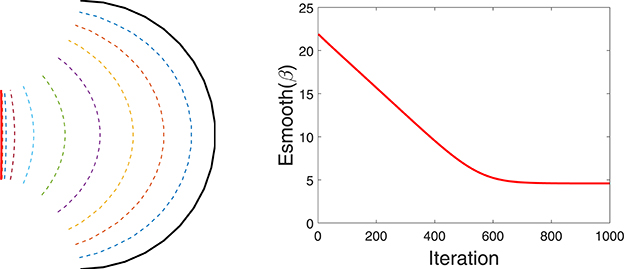
Figure 3. Evolution of a curve using negative gradient of E_smooth. (Left) The initial curve in black, intermediate curves as dotted lines, and the final curve in red. (Right) The evolution of E_smooth.

2.3. Atlas-Based Shape Prior

The next term to consider is E_prior that forces the shapes of estimated fiber tracts to be similar to certain desired shapes. This term encodes the prior shape information about fibers connecting two ROIs, and is based on a statistical model that is learnt from the training or atlas data (generated by current local or global methods). In a brain connectome study framework, the brain is generally pre-segmented into small anatomical regions using software such as Freesurfer and ANTs (Avants et al., 2011), and fibers connecting two ROIs are extracted. However, due to differences in sizes, orientations, and coordinate systems, these fibers connecting the same ROIs across subjects can not be directly used as prior for future fiber tractography. Removing these nuisance variable requires a formal definition of shape and shape space, and then one needs to develop a statistical model on this mathematical representation. Here we use elastic shape analysis developed in Srivastava and Klassen (2016) to represent and model fiber shapes. Specifically, we define ${S}$, the shape space of all curves in D and impose a truncated wrapped normal distribution on this space to reach a statistical shape model. The parameters of this model are estimated a priori from the training or atlas data. We present a brief summary of the elastic shape analysis here and refer the reader to the textbook (Srivastava and Klassen, 2016) for more details. For a curve β : [0, 1] → D, define $q(t)=\dot{\beta }(t)/\sqrt{\left|\dot{\beta }(t)\right|}$ be the square-root velocity function (SRVF) of β. This SRVF representation has an important property that a re-parameterization invariant Riemannian metric on the space of curves becomes the simple 𝕃² metric under transformation. As a corollary, for any q₁, q₂ ∈ 𝕃², we have ‖(q₁, γ) − (q₂, γ)‖ = ‖q₁ − q₂‖, for any γ ∈ Γ, where Γ is the set of all orientation preserving diffeomorphisms of [0, 1]. Here (q, γ) stands for $(q\circ \gamma )\sqrt{\stackrel{·}{\gamma }}$, representing the SRVF of the re-parameterized curve β ∘ γ. If we rotate β by O ∈ SO(2), we get O*β, and the corresponding SRVF is given by O*q.

Let β be a rescaled fiber curve such that it has unit length and let q be its SRVF. We define an orbit in the SRVF space as $\left[q\right]=\left\{O(q\circ \gamma )\sqrt{\stackrel{·}{\gamma }}|O\in SO(2),\gamma \in \Gamma \right\}$, which denotes an equivalence class representing a shape. Let ${S}$ be the set of all such equivalence classes; ${S}$ is called the shape space. The term E_prior in the active contour model is a function of β, but our statistical models are built on ${S}$ such that E_prior can effectively encode the shape information and be invariant to the different sizes and coordinate systems of different brains. However, ${S}$ is a nonlinear manifold space. To build a statistical model on ${S}$, we need some elementary tools such as efficient methods to calculate the mean and covariance matrix for a given set of data. Here we employ Karcher mean to calculate the mean shape of given fiber curves and the covariance matrix is calculated on the tangent space of ${S}$ at the estimated Karcher mean denoted by T_[μ](${S}$). The reader can refer to Srivastava et al. (2011) for the explicit procedures to calculate the Karcher mean and the covariance matrix.

Given a set of prior training shapes {[q_i], i = 1, …n} in ${S}$, let us assume that we have computed their Karcher mean [μ] and covariance K. We define the prior shape model using a truncated wrapped-normal density, which is estimated from the data as follows. First, obtain the singular value decomposition of K as [U, S, V] = svd(K), and let U_m be the m-dimensional principal subspace of $T_{\left[\mu \right]}({S})$ spanned by the first m columns of U. The shape prior distribution is defined as a wrapping of the truncated normal distribution mapped from U_m to ${S}$ using the exponential map. The truncated normal density on U_m is:

$\begin{array}{ll}v~\frac{1}{Z}{e}^{-\frac{1}{2}\left(v_{\Vert }^T{S}_m^{-1}{v}_{\Vert }+\Vert v_{\perp }{\Vert }^2/{\delta }^2\right)}{1}_{\Vert v\Vert <\pi },& (6)\end{array}$

where $v={exp}_{\left[\mu \right]}^{-1}(\left[q\right])$, $v_{\left|\right|}=U_m^{T}v$ is the projection of v into U_m, v_⊥ = v − U_mv_‖, S_m is the diagonal matrix containing the first m singular values, and Z is the normalizing constant. The scalar value δ is chosen to be less than the smallest singular value in S_m. Suppose now that we have a test shape [q] that represents a fiber tract during optimization process, and $v={exp}_{\left[\mu \right]}^{-1}(\left[q\right])$ be the shooting vector from the mean [μ] to [q]. Now define E_prior(q) to be the negative of the exponent in the shape prior given by Equation (6). That is, define $E_{prior}(q)=\frac{1}{2}{v}^T(U_m{S}_m^{-1}{U}_m^T)v+\frac{1}{2{\delta }^2}\left|\right|v-U_m{U}_m^{T}v|{|}^2$. Minimizing this functional is, therefore, equivalent to maximizing the likelihood of q under the chosen shape model. The gradient of E_prior with respect to v is equal to w = Av, where A is the matrix $A=U_m{S}_m^{-1}{U}_m^T+(I-U_m{U}_m^T)/{\delta }^2$. Notice that w is defined on the tangent space at μ rather than at q, so the final step is to parallel translate w from μ to q. Denote this parallel translation as $\bar{w}={\nabla }_q{E}_{prior}(q)$. An evolution of q along the negative gradient direction will result in an energy minimization precisely at the mean μ. The translated shooting vector $\bar{w}$ now represent the gradient of E_prior with respect to q. As the last step, this gradient is converted to ∇_βE_prior(β) using a numerical approximation.

Figure 4 shows a simple example of evolving a curve according to E_prior. The left panel shows the initial curve, and its updates using the negative gradient of E_prior. The corresponding decrease in E_prior is plotted on the right.

FIGURE 4

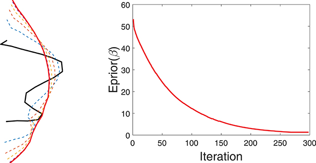
Figure 4. Evolution of a curve using negative gradient of E_prior. (Left) The initial curve in black, intermediate curves as dotted lines, and the final curve in red. (Right) The evolution of E_prior.

3. Bayesian Tractography Algorithm

When we put together the three components of the energy, the shape of β is controlled by gradients of E_data, E_prior and E_smooth, the smoothness is controlled by E_prior and E_smooth, and the nuisance variables (placement, scale, and rotation) are controlled only by E_data. Now we summarize the overall algorithm for Bayesian tractography using the tensor field (Algorithm 1).

ALGORITHM 1

Algorithm 1: Bayesian Tractography Using Geometric Shape Priors

The advantage of the proposed framework is that it uses a global optimization to overcome issues such as fiber crossing and spatial noise. The final tracking result depends not only on the diffusion data, but also on prior shape information. The inclusion of shape prior distinguishes our method from other energy minimization based fiber-tracking algorithms, and is essential for the optimization procedure to come out of local solutions and reach a global solution. Most importantly, in our framework, the brain is parcellated into small regions, and the shapes of fibers connecting any pair of regions are found to be consistent. The proposed truncated wrapped-normal distribution can effectively capture the variation of shapes for each connection in the training data. In addition, since we reconstruct the whole fiber simultaneously by minimizing an energy function, the issue of fiber crossing has almost no detrimental effect of our fiber tracking algorithm.

As stated earlier, this Bayesian approach requires either a the training data or an atlas of fiber tracts between regions of interest, to estimate shape model and develop E_prior. We can construct such data using existing tractography algorithms with maybe human inspection for quality control. However, since such a construction is needed only once, it can be performed offline.

4. Experimental Results

In this section we present some results using both simulated and real data to illustrate the performance of the proposed method.

4.1. Simulated 2-D Tensor Data

We first study our proposed tracking algorithm in the simulated settings. Let domain D = [0, 1]² for all our simulation examples. The tensor field on D, denoted by M:D→${P}$, is generated using certain fibers that play the role of ground truth. We discretize the domain D into a 20 × 20 grid, and the tensor within each grid is decided by the tangent directions of the line segments within this grid. In addition, a 2D Gaussian smoothing is applied to smooth the tensor field before applying our algorithm.

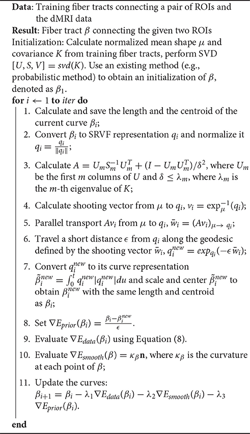
In the experiment presented in Figure 5, we use the blue lines as ground truth fiber tracts and generate a tensor field as shown in these panels. Then, using this tensor data, we estimate the fiber tracts using our and other methods, and the results are shown in red lines. On the left side we show results from standard streamline tractography, using starting points on one end. Due to a crossing of fibers in the middle, these tracts get diverted and sent to wrong directions. In the middle panel, we show results from our method but without using the shape prior term. This time the end points of the tracts are correct (by initialization) but some of the fibers don't quite reach the desired shape. Finally, we optimize fiber tracts using the full energy functional, including the shape prior, and display these results in the right panel. By including all the three terms, we overcomed issues caused by fiber crossing and local noise, and reached correct global structures. To better evaluate the tractography results, we calculate the distance between reconstructed fibers and ground truth using the L₂ norm. We first calculate the distance of each fiber from the ground truth and then use the mean of all distances to quantify the difference between reconstructed fiber bundle and ground truth fiber bundle. The distances for each method are given in Figure 5.

FIGURE 5

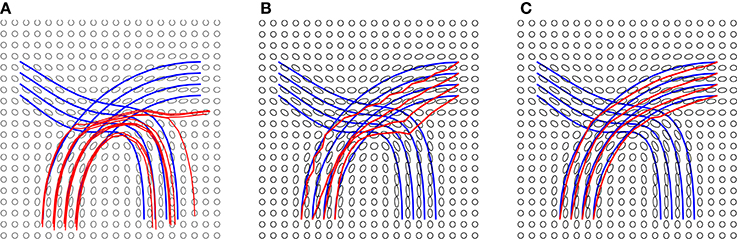
Figure 5. Tractography results on a simulated tensor field and distances from ground truth: (A) Streamline tractography from either region, d = 1.5e − 2, (B) our method without a shape prior, d = 2.2e − 3, and (C) our method with a shape prior, d = 3e − 4. The details of the prior are presented in Figure 6.

Additional details of this simulation experiment are presented in Figure 6, which shows evolution of a single fiber under E_total. The left panel shows the initial curve (black), the final curve (red), and the ground truth curve (blue). The right panel shows the evolution E_total during this iteration. In this experiment, we used the weights λ₁ = 0.8, λ₂ = 0.1, and λ₃ = 0.1.

FIGURE 6

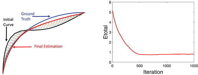
Figure 6. Detailed tractography results in the simulation example. Here we only focus on reconstruction of one of the curves. The black line is initialization, the red line is our result and the blue line is the ground truth.The right panel shows the evolution of the energy function.

4.2. Experiments Using Real Data

Next, we apply our method to some real datasets—dMRI images downloaded from the Human Connectome Project (HCP) (Van Essen et al., 2012). HCP contains about 900 subjects with diffusion MRI, but here we have used only 30 subjects for our experiments. The dMRI images in HCP has an isotropic resolution of 1.25 mm. To estimate a diffusion tensor at each voxel, we use the open source software Dipy (Garyfallidis et al., 2014). Figure 7A shows one slice of the 3 × 3 diffusion tensors estimated from a randomly selected dMRI image in HCP; a zoom-in of a small part of the image is shown on its right. Since in this paper we restrict to a 2D domain to illustrate our idea, we convert 3 × 3 diffusion tensors in the original data to 2 × 2 tensors by removing the diffusion directions perpendicular to the 2D slice plane. Figure 7B shows an example of this projection and shows the 2D tensors in form of their level sets or ellipses at each pixel location.

FIGURE 7

Figure 7. An example of a sagittal slice of diffusion tensor data. (A) Original data. (B) Projected 2D data.

In the results presented here, we focus on estimating a set of fiber curves connecting the left and right superior frontal gyri. In order to generate a prior shape model, we use tracts extracted for 30 subjects between these regions as the training dataset. These tracts were manually identified with the help of Freesurfer Destrieux Atlas (Destrieux et al., 2010) and the fiber curves built using the FACT method. These fibers are displayed on the left side of Figure 8. The Karcher mean μ of these fibers in the shape space ${S}$ is shown in the middle panel and the five dominant principal components of the Karcher covariance are displayed in the right panel. These dominant directions are computed by projecting the given shapes [q_i] in the tangent space T_[μ](${S}$) using the inverse exponential map, i.e., $v_i={exp}_{\left[\mu \right]}^{-1}(\left[q_i\right])$, and the computing principal components of the set {v_i} in the vector space T_[μ](${S}$). These principal directions, which as straight lines in T_[μ](${S}$) passing through [μ] in the middle, are then wrapped back on ${S}$ using the exponential maps. Each row of the right panel in Figure 8 shows plots one such direction, going from the largest variability to smallest from top to bottom.

FIGURE 8

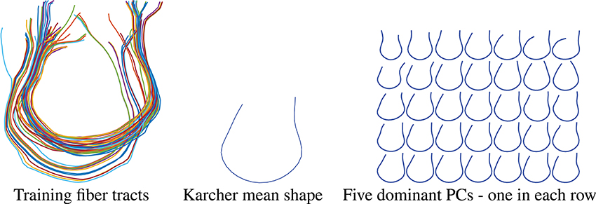
Figure 8. Thirty training samples of fiber tracts, their Karcher mean and principal directions of shape variation. The rightmost panel from top to bottom represents the first 5 principal directions of variation in the training data.

Having developed a prior model for fiber shapes from the training data, we then apply our Bayesian method to the tensor data, especially focusing on the areas where the streamline method fails, and the results are presented in Figure 9. We first show the results of the streamline method, using seeds from either ROI, in the first two panels. While the left panel in the top row gives an appearance that we have some fibers connecting the two ROIs, a closer look shows that this is actually not the case. In the middle panel we color the curves differently depending on which ROI is the seed located in. One can see that the set of curves—red and green—do not not reach the other ROI. They start from the ROI containing the seeds and diverge in the middle. This is in contradiction to the anatomical knowledge that the two regions are indeed connected through white matter fiber tracts. Using the proposed Bayesian technique, we obtained result shown in the rightmost panel of the top row. This picture shows an arbitrarily initialized curve drawn in blue, and the final estimated curve drawn in red color. The corresponding evolutions of the three energy terms—E_data, E_prior, and E_smooth—are shown in the middle row of this figure. Each one of these terms show a substantial decrease in their values during the iteration process.

FIGURE 9

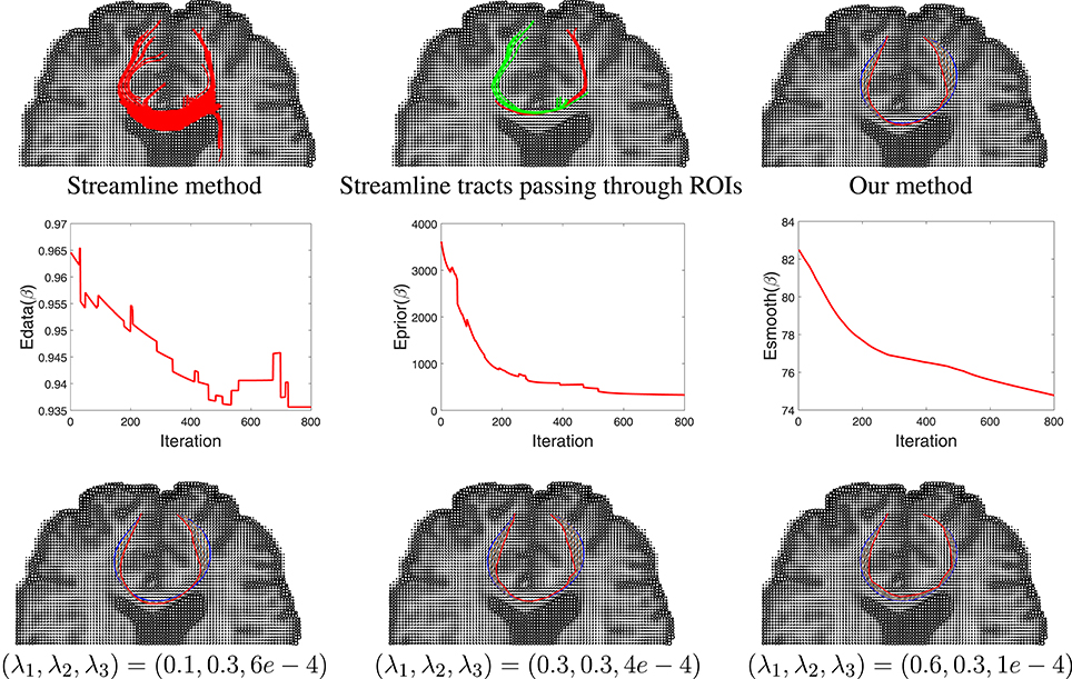
Figure 9. Results comparison between streamline method and our method. In the top row, the left panel shows the results using a streamline method, the middle panel shows some selected curves from that set that reach the two ROIs (different colors represent curves passing different regions), and the right panel shows tractography result using our Bayesian method. Here the blue line shows the initialization and red line is final result. The middle row shows the evolution of the three energy components in this estimation. The bottom row shows our tractography results under different weights of the energy components.

In order to study the impact of the weights λ₁, λ₂, and λ₃ on the final result, we generated estimates for a few different combinations of these weights. The results are shown in the last row of this figure. In case where the weight for shape prior is high, the final result is close to the prior mean. In contrast, when the weight for the data term is high, there is a better agreement between the curve and the tensor field.

Another example of this Bayesian estimation is presented in Figure 10 with similar settings. In this case the ROIs used are right hippocampus and right percentral.

FIGURE 10

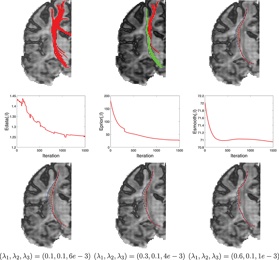
Figure 10. Another example similar to Figure 9.

4.3. Extension to Tractography Using HARDI Data

The proposed framework can be extended to HARDI data, where an ODF is used to better represent the underlying diffusion profile. The data term is now defined as:

$\begin{array}{ll}{E}_{data}[\beta ]={\displaystyle {\int }_0^1-}{f}_{\beta (t)}(n_{\beta }(t))dt,\text{ where }{n}_{\beta }(t)=\frac{\dot{\beta }(t)}{|\dot{\beta }(t)|}.& (7)\end{array}$

Here n_β(t) denotes the unit vector tangent to β at β(t) and f_p is the ODF at p ∈ D. The integrand is low at a location where the fiber tract is aligned with the ODF field and vice-versa. The next step is to derive the gradient of E_data with respect to β for use in gradient-based optimization. we can express the gradient of E_data as follows.

LEMMA 2. The gradient of E_data with respect to β, under the 𝕃² norm, is given by:

$\begin{array}{l}-\frac{{\dot{\beta }}^T(t)\ddot{\beta }(t)}{|\dot{\beta }(t){|}^3}\left(I-n_{\beta }(t)n_{\beta }^T(t)\right){\nabla }_{n_{\beta }}^T{f}_{\beta (t)}(n_{\beta }(t))-\frac{2}{|\dot{\beta }(t)|}{\dot{n}}_{\beta }(t)n_{\beta }^T(t){\nabla }_{n_{\beta }}^T{f}_{\beta (t)}(n_{\beta }(t))\\ +\frac{1}{|\dot{\beta }(t)|}\left(I-n_{\beta }(t)n_{\beta }^T(t)\right){\nabla }_{n_{\beta }}^2{f}_{\beta (t)}(n_{\beta }(t)){\dot{n}}_{\beta }(t).& (8)\end{array}$

A derivation of this expression is presented in the Appendix. We also show an experiment result on an ODF data in Figure 11. We use the blue lines as ground truth fiber tracts and generate ODF data as shown in Figure 11A. Under this ODF field, we estimate the fiber tracts using our method. The final reconstructed tracts are shown in red lines. In the middle panel, we show an evolution of a single fiber under E_total. In the right panel, we show the evolution E_total of each iteration.

FIGURE 11

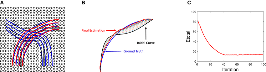
Figure 11. Tractography results on simulated ODF data. (A) Red lines are reconstructed fibers using our method and blue lines are the ground truth used to generate the ODF field. (B) Evaluation of one curve under our method. (C) Evolution of energy term E_total.

5. Conclusion and Discussion

This paper introduces a Bayesian approach for estimating fiber tracts, between given pairs of points in a human brain, using dMRI and HARDI data. The basic idea is to define a composite energy functional, using a linear combinations of terms that relate to data, curve smoothness, and a prior shape model, and then use the gradient of this energy to iteratively optimize a contour. There are several novelties in this setup: (1) the data term is locally scale-invariant and measures only the agreement of the fiber direction with the given diffusion tensor field, (2) the length of the fiber is kept as a separate term, in order to have an additional control over fiber size, and (3) an external term involving statistical shape models, of fibers tracts connecting given regions, is used to improve optimization and interpretability. These shape models can come from training data developed using manual interventions or population atlases established from previous studies. The gradients of all the terms have analytical forms, making the gradient-based optimization very efficient. This framework is demonstrated successfully using simulated 2D tensor fields and 2D slices of volume dMRI data.

One advantage of our method is that it can naturally handle crossing bundles since we construct the streamline as a whole object. Relying on the prior shape information, we can reconstruct a fiber curve that have similar geometry to the prior knowledge. Figure 12 illustrates one example that the proposed method is not sensitive to local fiber crossing. The blue lines are ground truth to generate the tensor field. From upper left to bottom left, more fibers were added to a region, which complicates the underlying tensor field. For the two selected regions, we initialize some black lines to connect them and the red lines are the final tractograhy results using our method. Those results indicates that our method can successfully reconstruct the fiber bundles in this challenge situation. The bottom right panel shows the shape prior that being used in our implementation.

FIGURE 12

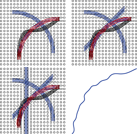
Figure 12. Examples showing that the proposed method can handle crossing and kissing fibers. Red lines are our tractograhy results, blue lines are ground truth and black lines are initializations. From upper left panel to bottom left panel, more and more crossing bundles are added into the simulation. The bottom right panel shows the shape prior used in our model.

However, the proposed Bayesian method needs to specify the starting and ending points for each extracted tract. To ensure that there is a tract between two ROIs, we currently rely on the atlas data. This procedure may end up with false positives, e.g., identifying a tract that does not exist. A future pruning procedure can be added as a post processing step, relying perhaps on the minimum energy as the reviewer has suggested. As another criterion, the diffusion profile along a tract can possibly be used as a feature to determine whether a tract is a false or a true positive.

As a future work, this framework can be naturally implemented using 3D dMRI data, and resulted tractography can be compared with some state of the art techniques.

Author Contributions

All authors listed, have made substantial, direct and intellectual contribution to the work, and approved it for publication. XD, ZZ, and AS have contributed in development of theory and computer implementation.

Conflict of Interest Statement

The authors declare that the research was conducted in the absence of any commercial or financial relationships that could be construed as a potential conflict of interest.

Acknowledgments

This research was supported in part by NSF grants DMS 1621787 and CCF 1617397 to AS. ZZ was partially supported by NSF grant DMS-1127914 to SAMSI. Data were provided in part by the HCP, WU-Minn Consortium (Principal Investigators: David Van Essen and Kamil Ugurbil; 1U54MH091657).

References

Avants, B. B., Tustison, N. J., Song, G., Cook, P. A., Klein, A., and Gee, J. C. (2011). A reproducible evaluation of ANTs similarity metric performance in brain image registration. NeuroImage 54, 2033–2044. doi: 10.1016/j.neuroimage.2010.09.025

PubMed Abstract | CrossRef Full Text | Google Scholar

Basser, P. J., Pajevic, S., Pierpaoli, C., Duda, J., and Aldroubi, A. (2000). In vivo fiber tractography using DT-MRI data. Magn. Reson. Med. 44, 625–632. doi: 10.1002/1522-2594(200010)44:4<625::AID-MRM17>3.0.CO;2-O

PubMed Abstract | CrossRef Full Text | Google Scholar

Behrens, T. E., Berg, H. J., Jbabdi, S., Rushworth, M. F., and Woolrich, M. W. (2007). Probabilistic diffusion tractography with multiple fibre orientations: what can we gain? Neuroimage 34, 144–155. doi: 10.1016/j.neuroimage.2006.09.018

PubMed Abstract | CrossRef Full Text | Google Scholar

Behrens, T. E., Woolrich, M., Jenkinson, M., Johansen-Berg, H., Nunes, R., Clare, S., et al. (2003). Characterization and propagation of uncertainty in diffusion-weighted mr imaging. Magn. Reson. Med. 50, 1077–1088. doi: 10.1002/mrm.10609

PubMed Abstract | CrossRef Full Text | Google Scholar

Bryner, D., Srivastava, A., and Huynh, Q. (2013). Elastic shape models for improving segmentation of object boundaries in synthetic aperture sonar images. Comput. Vis. Image Understand. 117, 1695–1710. doi: 10.1016/j.cviu.2013.07.001

CrossRef Full Text | Google Scholar

Cheng, G., Salehian, H., Forder, J., and Vemuri, B. C. (2015). Tractography from HARDI using an intrinsic unscented kalman filter. IEEE Trans. Med. Imaging 34, 298–305. doi: 10.1109/TMI.2014.2355138

PubMed Abstract | CrossRef Full Text | Google Scholar

Cheng, H., Wang, Y., Sheng, J., Kronenberger, W. G., Mathews, V. P., Hummer, T. A., et al. (2012). Characteristics and variability of structural networks derived from diffusion tensor imaging. Neuroimage 61, 1153–1164. doi: 10.1016/j.neuroimage.2012.03.036

PubMed Abstract | CrossRef Full Text | Google Scholar

Christiaens, D., Reisert, M., Dhollander, T., Maes, F., Sunaert, S., and Suetens, P. (2014). “Atlas-guided global tractography: imposing a prior on the local track orientation,” in Computational Diffusion MRI (Cambridge, MA: Springer), 115–123.

Google Scholar

Cook, P. A., Zhang, H., Awate, S. P., and Gee, J. C. (2008). “Atlas-guided probabilistic diffusion-tensor fiber tractography,” in Biomedical Imaging: From Nano to Macro, 2008. ISBI 2008. 5th IEEE International Symposium on (Paris: IEEE), 951–954. doi: 10.1109/ISBI.2008.4541155

CrossRef Full Text | Google Scholar

de Reus, M. A., and van den Heuvel, M. P. (2013). The parcellation-based connectome: limitations and extensions. Neuroimage 80, 397–404. doi: 10.1016/j.neuroimage.2013.03.053

PubMed Abstract | CrossRef Full Text | Google Scholar

Descoteaux, M. (2015). “High Angular Resolution Diffusion Imaging (HARDI),” in Wiley Encyclopedia of Electrical and Electronics Engineering, ed J. G. Webster (John Wiley & Sons, Inc.), 1–25. doi: 10.1002/047134608X.W8258

CrossRef Full Text | Google Scholar

Destrieux, C., Fischl, B., Dale, A., and Halgren, E. (2010). Automatic parcellation of human cortical gyri and sulci using standard anatomical nomenclature. Neuroimage 53, 1–15. doi: 10.1016/j.neuroimage.2010.06.010

PubMed Abstract | CrossRef Full Text | Google Scholar

Duncan, J. S., Papademetris, X., Yang, J., Jackowski, M., Zeng, X., and Staib, L. H. (2004). Geometric strategies for neuroanatomic analysis from MRI. Neuroimage 23, S34–S45. doi: 10.1016/j.neuroimage.2004.07.027

PubMed Abstract | CrossRef Full Text | Google Scholar

Durante, D., and Dunson, D. B. (2017). Bayesian inference and testing of group differences in brain networks. Bayesian Anal. doi: 10.1214/16-BA1030. [Epub ahead of print].

CrossRef Full Text | Google Scholar

Eckstein, I., Shattuck, D. W., Stein, J. L., McMahon, K. L., de Zubicaray, G., Wright, M. J., et al. (2009). Active fibers: matching deformable tract templates to diffusion tensor images. Neuroimage 47, T82–T89. doi: 10.1016/j.neuroimage.2009.01.065

PubMed Abstract | CrossRef Full Text | Google Scholar

Faugeras, O., Adde, G., Charpiat, G., Chefd'Hotel, C., Clerc, M., Deneux, T., et al. (2004). Variational, geometric, and statistical methods for modeling brain anatomy and function. NeuroImage 23, S46–S55. doi: 10.1016/j.neuroimage.2004.07.015

PubMed Abstract | CrossRef Full Text | Google Scholar

Fornito, A., Zalesky, A., and Breakspear, M. (2013). Graph analysis of the human connectome: promise, progress, and pitfalls. Neuroimage 80, 426–444. doi: 10.1016/j.neuroimage.2013.04.087

PubMed Abstract | CrossRef Full Text | Google Scholar

Friman, O., Farneback, G., and Westin, C.-F. (2006). A bayesian approach for stochastic white matter tractography. IEEE Trans. Med. Imaging 25, 965–978. doi: 10.1109/TMI.2006.877093

PubMed Abstract | CrossRef Full Text | Google Scholar

Fuster, A., Tristan-Vega, A., Haije, T. D., Westin, C.-F., and Florack, L. (2014). “A novel Riemannian metric for geodesic tractography in DTI,” in Computational Diffusion MRI and Brain Connectivity (Nagoya: Springer), 97–104. doi: 10.1007/978-3-319-02475-2_9

CrossRef Full Text | Google Scholar

Garyfallidis, E., Brett, M., Amirbekian, B., Rokem, A., van der Walt, S., Descoteaux, M., et al. (2014). Dipy, a library for the analysis of diffusion MRI data. Front. Neuroinform. 8:8. doi: 10.3389/fninf.2014.00008

PubMed Abstract | CrossRef Full Text | Google Scholar

Hagmann, P., Thiran, J. P., Jonasson, L., Vandergheynst, P., Clarke, S., Maeder, P., et al. (2003). DTI mapping of human brain connectivity: statistical fibre tracking and virtual dissection. Neuroimage 19, 545–554. doi: 10.1016/S1053-8119(03)00142-3

PubMed Abstract | CrossRef Full Text | Google Scholar

Hao, X., Zygmunt, K., Whitaker, R. T., and Fletcher, P. T. (2014). Improved segmentation of white matter tracts with adaptive Riemannian metrics. Med. Image Anal. 18, 161–175. doi: 10.1016/j.media.2013.10.007

PubMed Abstract | CrossRef Full Text | Google Scholar

Joshi, S. H., and Srivastava, A. (2009). Intrinsic Bayesian active contours for extraction of object boundaries in images. Int. J. Comput. Vis. 81, 331–355. doi: 10.1007/s11263-008-0179-8

PubMed Abstract | CrossRef Full Text | Google Scholar

Kichenassamy, S., Kumar, A., Olver, P., Tannenbaum, A., and Yezzi, A. (1995). “Gradient flows and geometric active contour models,” in Fifth ICCV (Cambridge, MA), 810–815. doi: 10.1109/ICCV.1995.466855

CrossRef Full Text | Google Scholar

Lankton, S., Melonakos, J., Malcolm, J., Dambreville, S., and Tannenbaum, A. (2008). “Localized statistics for DW-MRI fiber bundle segmentation,” in Computer Vision and Pattern Recognition Workshops, 2008. CVPRW'08. IEEE Computer Society Conference on (Anchorage, AK: IEEE), 1–8.

PubMed Abstract | Google Scholar

Lenglet, C., Deriche, R., and Faugeras, O. (2004). “Inferring white matter geometry from diffusion tensor MRI: Application to connectivity mapping,” in European Conference on Computer Vision (Berlin; Heidelberg: Springer), 127–140. doi: 10.1007/978-3-540-24673-2_11

CrossRef Full Text | Google Scholar

Li, W., and Hu, X. (2013). Robust tract skeleton extraction of cingulum based on active contour model from diffusion tensor MR imaging. PLoS ONE 8:e56113. doi: 10.1371/journal.pone.0056113

PubMed Abstract | CrossRef Full Text | Google Scholar

Maier-Hein, K., Neher, P., Houde, J.-C., Cote, M.-A., Garyfallidisand, E., Zhong, J., et al. (2016). Tractography-based connectomes are dominated by false-positive connections. biorxiv.

Google Scholar

Melonakos, J. (2009). Geodesic Tractography Segmentation for Directional Medical Image Analysis. Atlanta, GA: ProQuest.

Google Scholar

Melonakos, J., Pichon, E., Angenent, S., and Tannenbaum, A. (2008). Finsler active contours. IEEE Trans. Patt. Anal. Mach. Intell. 30, 412–423. doi: 10.1109/TPAMI.2007.70713

PubMed Abstract | CrossRef Full Text | Google Scholar

Mohan, V., Melonakos, J., Niethammer, M., Kubicki, M., and Tannenbaum, A. R. (2009). Finsler Level Set Segmentation for Imagery in Oriented Domains. Georgia Institute of Technology.

Google Scholar

Mori, S., Crain, B. J., Chacko, V. P., and van Zijl, P. C. (1999). Three-dimensional tracking of axonal projections in the brain by magnetic resonance imaging. Ann. Neurol. 45, 265–269. doi: 10.1002/1531-8249(199902)45:2<265::AID-ANA21>3.0.CO;2-3

PubMed Abstract | CrossRef Full Text | Google Scholar

Mori, S., and van Zijl, P. C. (2002). Fiber tracking: principles and strategies - a technical review. NMR Biomed. 15, 468–480. doi: 10.1002/nbm.781

PubMed Abstract | CrossRef Full Text | Google Scholar

Mori, S., Wakana, S., Nagae-Poetscher, L., and van Zijl, P. (2005). MRI Atlas of Human White Matter, 1st Edn. Baltimore, MD: Elsevier.

O'Donnell, L., Haker, S., and Westin, C. (2002). “New approaches to estimation of white matter connectivity in diffusion tensor MRI: elliptic PDEs and geodesics in a tensor-warped space,” in Proceedings of Medical Imaging, Computing and Computer Assisted Intervention, Lecture Notes in Computer Science, Vol. 2488 (Berlin: Springer), 459–466.

Pichon, E., Westin, C.-F., and Tannenbaum, A. R. (2005). “A hamilton-jacobi-bellman approach to high angular resolution diffusion tractography,” in International Conference on Medical Image Computing and Computer-Assisted Intervention (Berlin; Heidelberg: Springer), 180–187.

Google Scholar

Reisert, M., Mader, I., Anastasopoulos, C., Weigel, M., Schnell, S., and Kiselev, V. (2011). Global fiber reconstruction becomes practical. Neuroimage 54, 955–962. doi: 10.1016/j.neuroimage.2010.09.016

PubMed Abstract | CrossRef Full Text | Google Scholar

Srivastava, A., and Klassen, E. (2016). Functional and Shape Data Analysis. New York, NY: Springer-Verlag. doi: 10.1007/978-1-4939-4020-2

CrossRef Full Text | Google Scholar

Srivastava, A., Klassen, E., Joshi, S., and Jermyn, I. (2011). Shape analysis of elastic curves in Euclidean spaces. IEEE Trans. Patt. Anal. Mach. Intell. 33, 1415–1428. doi: 10.1109/TPAMI.2010.184

PubMed Abstract | CrossRef Full Text | Google Scholar

Van Essen, D. C., Ugurbil, K., Auerbach, E., Barch, D., Behrens, T. E., Bucholz, R., et al. (2012). The human connectome project: a data acquisition perspective. NeuroImage 62, 2222–2231. doi: 10.1016/j.neuroimage.2012.02.018

PubMed Abstract | CrossRef Full Text | Google Scholar

Yap, P.-T., Gilmore, J. H., Lin, W., and Shen, D. (2011). “Longitudinal tractography with application to neuronal fiber trajectory reconstruction in neonates,” in International Conference on Medical Image Computing and Computer-Assisted Intervention (Berlin; Heidelberg: Springer), 66–73.

Google Scholar

Zach, C., Shan, L., and Niethammer, M. (2009). “Globally optimal finsler active contours,” in Joint Pattern Recognition Symposium (Jena: Springer), 552–561. doi: 10.1007/978-3-642-03798-6_56

CrossRef Full Text | Google Scholar

Appendix

Lemma 1

In this section we derive an expression for the gradient of E_data[β] with respect to β. Let h ∈ ${B}$ be a perturbation to the curve β such that it is zero at the boundaries, i.e., h : [0, 1] → ℝ² and h(0) = h(1) = 0. Since, $E_{data}\left[\beta +ϵh\right]={\int }_0^1{n}_{\beta +ϵh}^T(t)M_{\beta (t)+ϵh(t)}^{-1}{n}_{\beta +ϵh}^T(t)dt$, the directional derivative of E_data in the direction of h is given by:

$\begin{array}{l}\frac{d}{d\epsilon }{|}_{\epsilon =0}{E}_{data}[\beta +\epsilon h]={\displaystyle {\int }_0^1(2n_{\beta }^T(t)}{M}_{\beta (t)}^{-1}{u}_{\beta ,h}(t)\\ +n_{\beta }^T(t)\langle \langle {\nabla }_x{M}_{\beta (t)}^{-1},h(t)\rangle \rangle n_{\beta }(t))dt,\end{array}$

where: $u_{\beta ,h}(t)=\frac{d}{dϵ}{|}_{ϵ=0}(n_{\beta +ϵh}(t))=\frac{1}{|\dot{\beta }(t)|}(I-n_{\beta }(t)n_{\beta }^T(t))ḣ(t)\equiv A_{\beta }(t)ḣ(t)$. The last equality is used to define A_β(t). We simplify the two terms one by one:

• First Term: Using integration by parts and using the boundary conditions h(0) = h(1) = 0, the first term becomes:

$\begin{array}{l}{\displaystyle {\int }_0^{1}2}{n}_{\beta }^T(t)M_{\beta (t)}^{-1}{u}_{\beta ,h}(t)dt={\displaystyle {\int }_0^{1}2}{n}_{\beta }^T(t)M_{\beta }^{-1}(t)A_{\beta (t)}\dot{h}(t))dt\\ =-{\displaystyle {\int }_0^1\langle }2\frac{d}{dt}\left(A_{\beta (t)}{M}_{\beta (t)}^{-1}{n}_{\beta }(t)\right)h(t)\rangle dt\end{array}$

Here

$\begin{array}{l}\frac{d}{dt}\left(A_{\beta (t)}{M}_{\beta (t)}^{-1}{n}_{\beta }(t)\right)=\frac{d}{dt}\left(\frac{1}{|\dot{\beta }(t)|}\left(I-n_{\beta }(t)n_{\beta }^T(t)\right)M_{\beta (t)}^{-1}{n}_{\beta }(t)\right)\\ =\frac{1}{|\dot{\beta }(t)|}\left(M_{\beta (t)}^{-1}{\dot{n}}_{\beta }(t)+\langle \langle {\nabla }_x{M}_{\beta (t)}^{-1},\dot{\beta }(t)\rangle \rangle n_{\beta }(t)\right)-\frac{{\dot{\beta }}^T(t)\ddot{\beta }(t)}{|\dot{\beta }(t){|}^3}{M}_{\beta (t)}^{-1}{n}_{\beta }(t)\\ -\frac{1}{|\dot{\beta }(t)|}\left({\dot{n}}_{\beta }(t)n_{\beta }^T(t)M_{\beta (t)}^{-1}{n}_{\beta }(t)+n_{\beta }(t)n_{\beta }^T(t)\langle \langle {\nabla }_x{M}_{\beta (t)}^{-1}\dot{\beta }(t)\rangle \rangle n_{\beta }(t)+2n_{\beta }(t)n_{\beta }^T(t)M_{\beta (t)}^{-1}{\dot{n}}_{\beta }(t)\right)\\ +\frac{{\dot{\beta }}^T(t)\ddot{\beta }(t)}{|\dot{\beta }(t){|}^3}{n}_{\beta }(t)n_{\beta }^T(t)M_{\beta (t)}^{-1}{n}_{\beta }(t),\text{ where }{\dot{n}}_{\beta }(t)=\frac{d}{dt}{n}_{\beta }(t)=\frac{\ddot{\beta }(t)}{|\dot{\beta }(t)|}-\frac{\dot{\beta }(t){\dot{\beta }}^T(t)\ddot{\beta }(t)}{|\dot{\beta }(t){|}^3}.\end{array}$

• Second Term: The second term can be rearranged as:

$\begin{array}{l}{\displaystyle {\int }_0^1\langle \langle \langle tran({\nabla }_x{M}_{\beta (t)}^{-1})n_{\beta }(t)n_{\beta }(t),h(t)\rangle \rangle }dt\end{array}$

where $tran({\nabla }_x{M}_{\beta (t)}^{-1})$ is transpose of ${\nabla }_x{M}_{\beta (t)}^{-1}$.

Thus, the full gradient of E_data with respect to β is given by:

$\begin{array}{l}-2\{\frac{1}{|\dot{\beta }(t)|}\left(M_{\beta (t)}^{-1}{\dot{n}}_{\beta }(t)+\langle \langle {\nabla }_x{M}_{\beta (t)}^{-1},\dot{\beta }(t)\rangle \rangle n_{\beta }(t)\right)-\frac{{\dot{\beta }}^T(t)\ddot{\beta }(t)}{|\dot{\beta }(t){|}^3}{M}_{\beta (t)}^{-1}{n}_{\beta }(t)\\ -\frac{1}{|\dot{\beta }(t)|}\left({\dot{n}}_{\beta }(t)n_{\beta }^T(t)M_{\beta (t)}^{-1}{n}_{\beta }(t)+n_{\beta }(t)n_{\beta }^T(t)\langle \langle {\nabla }_x{M}_{\beta (t)}^{-1}\dot{\beta }(t)\rangle \rangle n_{\beta }(t)+2n_{\beta }(t)n_{\beta }^T(t)M_{\beta (t)}^{-1}{\dot{n}}_{\beta }(t)\right)\\ +\frac{{\dot{\beta }}^T(t)\ddot{\beta }(t)}{|\dot{\beta }(t){|}^3}{n}_{\beta }(t)n_{\beta }^T(t)M_{\beta (t)}^{-1}{n}_{\beta }(t)\}+\langle \langle tran({\nabla }_x{M}_{\beta (t)}^{-1}),n_{\beta }(t)\rangle \rangle n_{\beta }(t).\end{array}$

Lemma 2

Let's denote f_p as the ODF at p ∈ D and for simplicity, f(t) will be used to denote f_β(t)(n_β(t)) in the following derivation. In this section we derive an expression for the gradient of E_data[β] with respect to β. Let h ∈ ${B}$ be a perturbation to the curve β such that it is zero at the boundaries, i.e., h : [0, 1] → ℝ² and h(0) = h(1) = 0. Since, $E_{data}\left[\beta +ϵh\right]={\int }_0^{1}f(n_{\beta +ϵh}(t))dt$, the directional derivative of E_data in the direction of h is given by:

$\begin{array}{l}\frac{d}{d\epsilon }{|}_{\epsilon =0}{E}_{data}[\beta +\epsilon h]={\displaystyle {\int }_0^1{\nabla }_{n_{\beta }}}f(t)u_{\beta ,h}(t)dt,\end{array}$

where: $u_{\beta ,h}(t)=\frac{d}{dϵ}{|}_{ϵ=0}(n_{\beta +ϵh}(t))=\frac{1}{|\dot{\beta }(t)|}(I-n_{\beta }(t)n_{\beta }^T(t))ḣ(t)\equiv A_{\beta }(t)ḣ(t)$. Using integration by parts and using the boundary conditions h(0) = h(1) = 0, the term becomes:

$\begin{array}{l}{\displaystyle {\int }_0^1{\nabla }_{n_{\beta }}}f(t)u_{\beta ,h}(t)dt={\displaystyle {\int }_0^1{\nabla }_{n_{\beta }}}f(t)A_{\beta (t)}\dot{h}(t))dt=-{\displaystyle {\int }_0^1\langle }\frac{d}{dt}\left(A_{\beta }(t){\nabla }_{n_{\beta }}^{T}f(t)\right)h(t)\rangle dt\end{array}$

Here

$\begin{array}{l}\frac{d}{dt}\left(A_{\beta (t)}{\nabla }_{n_{\beta }}^{T}f(t)\right)=\frac{d}{dt}\left(\frac{1}{|\dot{\beta }(t)|}\left(I-n_{\beta }(t)n_{\beta }^T(t)\right){\nabla }_{n_{\beta }}^{T}f(t)\right)\\ =-\frac{{\dot{\beta }}^T(t)\ddot{\beta }(t)}{|\dot{\beta }(t){|}^3}\left(I-n_{\beta }(t)n_{\beta }^T(t)\right){\nabla }_{n_{\beta }}^{T}f(t)-\frac{2}{|\dot{\beta }(t)|}{\dot{n}}_{\beta }(t)n_{\beta }^T(t){\nabla }_{n_{\beta }}^{T}f(t)\\ +\frac{1}{|\dot{\beta }(t)|}\left(I-n_{\beta }(t)n_{\beta }^T(t)\right){\nabla }_{n_{\beta }}^{2}f(t){\dot{n}}_{\beta }(t),\end{array}$

where ${\dot{n}}_{\beta }(t)=\frac{d}{dt}{n}_{\beta }(t)=\frac{\ddot{\beta }(t)}{|\dot{\beta }(t)|}-\frac{\dot{\beta }(t){\dot{\beta }}^T(t)\ddot{\beta }(t)}{|\dot{\beta }(t){|}^3}.$.

Thus, the full gradient of E_data with respect to β is given by:

$\begin{array}{l}-\frac{{\dot{\beta }}^T(t)\ddot{\beta }(t)}{|\dot{\beta }(t){|}^3}\left(I-n_{\beta }(t)n_{\beta }^T(t)\right){\nabla }_{n_{\beta }}^{T}f(t)-\frac{2}{|\dot{\beta }(t)|}{\dot{n}}_{\beta }(t)n_{\beta }^T(t){\nabla }_{n_{\beta }}^{T}f(t)+\frac{1}{|\dot{\beta }(t)|}\left(I-n_{\beta }(t)n_{\beta }^T(t)\right){\nabla }_{n_{\beta }}^{2}f(t){\dot{n}}_{\beta }(t).\end{array}$